Time-Reversal Symmetry Breaking and Spontaneous Anomalous Hall Effect in Fermi Fluids
Abstract
We study the spontaneous non-magnetic time-reversal symmetry breaking in a two-dimensional Fermi liquid without breaking either the translation symmetry or the charge symmetry. Assuming that the low-energy physics is described by fermionic quasiparticle excitations, we identified an “emergent” local symmetry in momentum space for an -band model. For a large class of models, including all one-band and two-band models, we found that the time-reversal and chiral symmetry breaking can be described by the gauge theory associated with this emergent local symmetry. This conclusion enables the classification of the time-reversal symmetry-breaking states as types and , depending on the type of accompanying spatial symmetry breaking. The properties of each class are studied. In particular, we show that the states breaking both time-reversal and chiral symmetries are described by spontaneously generated Berry phases. We also show examples of the time-reversal symmetry-breaking phases in several different microscopically motivated models and calculate their associated Hall conductance within a mean-field approximation. The fermionic nematic phase with time-reversal symmetry breaking is also presented and the possible realizations in strongly correlated models such as the Emery model are discussed.
pacs
71.10.Hf,11.30.Er,71.10.AyI introduction
In this paper we consider the effects of the spontaneous breaking of time-reversal () invariance in electronic systems. This is a problem of considerable current interest particularly in the context of strongly correlated systems. While the physics of strong correlation is important, many aspects of spontaneous time-reversal symmetry breaking are not well understood even at the level of weakly coupled systems, well described by Fermi-liquid theory. The problem that we will consider is that of the possible quantum phase transitions to states in which time-reversal invariance is spontaneously broken in electronic systems with several Fermi surfaces, and how to classify them.
One of the most important consequences of the spontaneous breaking of time reversal is that these ground states may exhibit a spontaneous (nonquantized) anomalous Hall effect. More specifically, we consider Fermi systems with multiple Fermi surfaces with condensates in the particle-hole channel that break time-reversal invariance. As a consequence, these systems have a nontrivial relative Fermi-surface Berry curvature which quantifies the strength of the time-reversal symmetry breaking. The theory that we present here has a close connection with Haldane’s analysis of the anomalous Hall effect as a Berry curvature on the Fermi surface. [1] The nontrivial new effect that results from these states is that they exhibit a spontaneous anomalous Hall effect, i.e., present even in the absence of extrinsic effects such as magnetic impurities or external magnetic fields.
Time-reversal symmetry breaking in the absence of external magnetic fields or spontaneous spin ordering has been a focus of interest in condensed-matter physics for quite some time, at least since the discovery of high superconductivity in the copper oxide materials. Quite early on it was postulated that frustrated two-dimensional (2D) quantum antiferromagnets may have “chiral spin liquid” phases (or ground states), translationally invariant states without magnetic long-range order.[2, 3, 4, 5] The known behavior of high superconductors does not appear to be consistent with a spin liquid ground state. The discovery of time-reversal symmetry-breaking effects in recent experiments on Sr2RuO4 and in underdoped YBa2Cu3O6+y (and similar systems) has renewed the interest in understanding time-reversal symmetry-breaking phases in strongly correlated electronic systems.
The main purpose of this paper is to inquire if it is in principle possible to have an electronic system with a nonmagnetic translationally invariant ground state that breaks spontaneously time-reversal invariance. Such a system would exhibit a spontaneous Hall effect and a Kerr effect even in the absence of disorder and/or magnetic fields. We will focus here on simple models of quantum phase transitions in electronic systems, without ferromagnetism or any other form of long-range magnetic order. We will further assume that these systems have well-defined electronic quasiparticle excitations and are hence extensions of Fermi-liquid theory. This assumption is valid for any mean-field approaches and as will be shown in Sec. VI, is valid even if the fluctuations of the order parameter around its mean-field value are considered for lattice models. We will see that, even in this “weak-coupling” approach, states with the desired properties are physically sensible. (Naturally, the naive applicability of the details of this theory to a regime of strong correlations, necessary in the context of the cuprates, is questionable.)
Within this weak-coupling approach, time-reversal breaking phases can be described in terms of properties of the resulting one-particle states and of their effective Fermi surfaces. Of particular importance is the fact that a system with Fermi surfaces obtains an “emergent” (and approximate) local gauge (in momentum space) symmetry near the Fermi-liquid fixed point.
In Sec. II we show that the natural way to represent this structure is in terms of an Abelian gauge theory of gauge fields. These gauge fields describe the quasiparticle Berry phases [6] in the sense discussed recently by Haldane. [1] For systems with one or two band(s), the structure of symmetry breaking is described by these gauge fields and the symmetry properties of the quasiparticle dispersion relation under space inversion. However, for more than two bands, more complex symmetry-breaking phases arise involving additional time-reversal breaking operators which are neither Berry connections nor the space inversion symmetry of the quasiparticle dispersion relations. Nevertheless, the Berry connections and the inversion symmetry of the quasiparticle dispersion relation still describe a large class of the symmetry-breaking states even in multiband models.
We will only consider the symmetry-breaking phases described by these gauge fields (Berry phases) and the inversion symmetry of quasiparticle dispersion relations. Within this constraint, the systems that we describe are invariant under the combined transformation of , where is the chiral transformation (i.e., a mirror reflection) and stands for space inversion. With the symmetry, the symmetry-breaking states can be classified into two classes, according to the accompanying or symmetry breaking. We refer to the states that preserve all three symmetries , , and , as the normal states. As for the symmetry-breaking states, if the inversion symmetry is also broken but the chiral and the combined symmetries are preserved, these states will be referred to as type . In contrast, the states that break and but preserve and will be referred as the type states. The states that break all three of , , and are considered as a mixing of types and . Obviously, type states have no Kerr or Hall effect, but type may have. The type state is somehow trivial if we notice that the momentum changes sign under or . Hence, in this paper, we mostly concentrate on the type states.
Using the Berry connections, we show that type phases may appear in one-band or multiband models. However, the type phases can only be found in multiband models. The phase transitions from the normal phase to the type phase can be classified into two different scenarios depending on whether the band structure has degeneracy points or not (degeneracy lines or areas usually require fine tuning and will not be considered).
After exploring the general theory, we use mean-field theory to investigate the symmetry breaking in several specific models. In Sec. III, we study the general symmetry properties of the (fermion bilinear) order parameters in the particle-hole channel for systems whose band structure contains no degeneracy point and show that the type symmetry-breaking states requires two order parameters.
In Sec. IV, we present a mean-field study of 2D Fermi liquids with continuous rotational and translational symmetries, and time-reversal invariance. In this section we discuss the possible patterns of spontaneous breaking of time-reversal invariance, inversion and chiral symmetries, and rotational invariance in interacting metallic systems. Although the models we discuss here use the framework of the Landau theory of the Fermi liquid, the patterns of symmetry breaking that are found, as well as the resulting phenomenology, are of more general interest. In a Landau-type model with four-fermion forward scattering interactions, analogous to the type discussed in Refs. [7] and [8], time-reversal symmetry-breaking phases can be stabilized and are usually accompanied by rotational symmetry breaking. In a one-band model, the type phases can be reached through a Pomeranchuk instability [9] in odd angular momentum channels (with angular momentum ), nematic-like phases with broken space inversion and time reversal. However for two-band models type phases may also appear, and have a similar structure to the phases in fermionic systems with spin described in Refs.[10] and [8]. In this section we construct the phase diagram. Here we also evaluate the Hall conductance for these phases, which is not quantized since these phases are gapless and conducting. We also show that the Hall conductance found here is related with a topological index ,the Kronecker index of the homotopy mappings , i.e., . This in turn implies that the symmetry breaking in these phases is stable against adiabatic perturbations, even though the actual value of the unquantized Hall conductance is not universal and can be changed continuously.
In Sec. V, we generalize these symmetry-breaking phases to lattice models and discuss subtle effects arising from the degeneracy points in the band structures. In particular we show that without degeneracy points, the time reversal and chiral symmetry-breaking phase can be reached from a normal Fermi liquid either by a direct first-order transition or by two separate phase transitions through an intermediate phase characterized by rotational symmetry breaking. But in the presence of degeneracy points, the direct transition between the and symmetry-breaking phase and the normal Fermi liquid may be second order.
Finally, in Sec. VII, we present a discussion of the experimental consequences of this work. The relation between this work and its particle-particle channel counterpart is also discussed, as well as the similarities and differences with the phases studied in Ref. [8]. We present details of the calculations for two-band models in Appendix A. The topological and physical meaning of the Wilson loops introduced in Sec. II is discussed in Appendix B. In Appendix C, we present the details of the calculation of the Hall conductivity, and in Appendix D, the symmetry of the and phases (to be defined below) is discussed.
II Gauge theory and Berry phase
In this section, we study the general properties of the spontaneous symmetry breaking for a fermionic system, which we will assume to be well described by an effective Fermi liquid, i.e., a fermionic system with well-defined quasiparticle excitations which are asymptotically free at low energies. We will also assume that time-reversal invariance is not broken explicitly and hence that there is neither an external magnetic field nor any sort of magnetic long-range order. We will consider systems without magnetic impurities, trapped magnetic fluxes, or other explicit extraneous time-reversal symmetry-breaking effects. For one- and two-band models, we will show that:
- 1.
The symmetry-breaking effects are represented either by the existence of Berry phases or by the symmetry properties of the quasiparticle dispersion relation under space inversion;
- 2.
There is a symmetry, where is time-reversal, is a chiral transformations (reflection across a suitable mirror plane), and is space inversion;
- 3.
In the absence of explicit breaking of , the total Berry phase of all the bands is zero, ;
- 4.
There is no type symmetry breaking in a one-band model;
- 5.
Degeneracy points of the effective band structure (defined later) have an associated quantized Berry flux , with integer ;
- 6.
Systems with and without degeneracy points have different properties when undergoing a phase transition to a type symmetry-breaking phase.
Here type (breaking and ) and type (breaking and ) refer to the two types of breaking phases discussed in the Introduction. For models with more than two bands, we will show that by assuming , all other conclusions above can be generalized easily.
The low-energy properties of a Fermi liquid are described by its spectrum of quasiparticle excitations, i.e., Bloch waves and their dispersion relation. The dispersion relation , where is the band index with for an band model, transforms to under time reversal or space inversion but is invariant under chirality or the simultaneous action of and . Hence, the odd part of the dispersion relation, , describes type symmetry breaking.
The Bloch waves may also contain information of the symmetry breaking. Due to the (perturbative) irrelevance at low energies of the quasiparticle interactions under the renormalization group (RG), [11] a Fermi liquid with bands is invariant under a gauge transformation
| (1) |
where is the Bloch wave function of the band . This gauge symmetry, associated with independent redefinitions (gauge transformations) of the phase of the quasiparticle Bloch states for each band at each wave vector , is an “emergent” symmetry, asymptotically accurate only close enough to the Fermi-liquid fixed point. Away from this fixed point, the irrelevant quasiparticle scattering processes make this symmetry an approximate one. This effect can be studied perturbatively as will be shown in Sec. IV.4, but can (and will) be ignored for the purposes of the present discussion.
To remove the redundant degrees of freedom, one defines the overlap matrix [12]
| (2) |
The diagonal terms, , are Berry connections which under the gauge transformation of Eq.(1) transform as gauge fields:
| (3) |
The off-diagonal terms, for , transform instead as
| (4) |
which cannot be regarded as gauge fields. Clearly the overlap matrix are the matrix elements of the position operator in Bloch states. [12] The diagonal terms are directly related with the “anomalous velocity” in the semiclassical theories of Bloch waves. [13]
It is well known from the theory of the Hall effect (see, for instance, Haldane’s work[1] and references therein) that an external magnetic field induces a nontrivial Berry curvature. This affects all the bands in essentially the same way. In what follows we will assume that time-reversal invariance is not broken explicitly by external fields. Thus, the total Berry curvature vanishes as required by Eq. (33).
We now restrict our discussion on symmetry breaking that can be described by the diagonal terms alone. As shown in Appendix A, this assumption is automatically satisfied for all one- and two-band models. For systems with three or more bands it is also possible to have phases that break time-reversal invariance which are described purely by off-diagonal operators, (with ). Even though they do break time-reversal, these states do not have a Berry phase and, consequently, will not have a spontaneous anomalous Hall effect. We will discuss in Sec. V that one of the so-called Varma loop states, in the notation of Ref.[14], is an example of a time-reversal symmetry-breaking state in a three-band model without an anomalous Hall effect.
From now on, only the diagonal terms will be considered. Their, gauge-invariant, physical degrees of freedom are described by the Wilson loops
| (5) | |||
| (6) |
which is also the Berry phase. [1] Notice that in principle one can consider any path in momentum space. In practice, for a gapless system the path of physical interest coincides with the location of the Fermi surfaces of the bands (see below).
Under the action of the chiral transformation , space inversion , and time reversal , the Wilson loops transform as
| (7) | |||
| (8) | |||
| (9) |
The chiral transformation reverses the orientation of the path, , and hence, it transforms into its complex conjugate. The space inversion operator changes momentum to , which changes the integration contour but preserves its direction. The time-reversal operator is antiunitary. It changes to as but also changes the Wilson loop to its complex conjugate, which is also how acts. Therefore, is invariant under . Since the dispersion relation is invariant under (and ), then the system must be invariant under . This is one of the key results of this paper, which makes the classification of the types and symmetry-breaking states possible.
As we noted above, in the absence of magnetic fields (and of any other explicit breaking of time reversal), there is a constraint over the total Berry phase,
| (10) |
which implies that there is no Berry phase associated with the charge sector, the overall gauge group. However, in the presence of magnetic fields, the phase of the Bloch wave cannot be determined in a unique and smooth way over the entire Brillouin zone. [15] This invalidates the assumptions behind Eq. (33), leading to a nontrivial Berry phase in the charge sector and a nonvanishing Hall conductance. On the other hand, in the absence of external magnetic fields, although the constraint of Eq. (10) prevents the charge sector to obtain a Berry phase, a nontrivial relative Berry phase between different bands is still allowed. This is the key point in our study of a spontaneous symmetry breaking without magnetic ordering that we are interested in here.
For a one-band model, the constraint that the total Berry phase must be trivial, , implies that the Wilson loops must be real, . Hence, the Wilson loop is an eigenvector of the chiral transformation , i.e., , and the symmetry always holds. Thus, for one-band models, only type time-reversal spontaneous symmetry breaking is allowed.
Let us consider now the case of two-band models which allow for a richer structure. In this case Eq.(10) now becomes . Hence, only one Berry phase (or equivalently ) is linearly independent. For a state with , or equivalently , symmetry (the normal state or the type state), again one obtains , which quantizes the Berry phase to be , with integer . Conversely, if and are broken, the symmetry breaking is type . In this case, symmetry breaking in two-band models can be described by obtaining an imaginary part. Equivalently, the Berry phase becomes nonquantized for a type time-reversal symmetry breaking.
The effective one-particle Hamiltonians of a two-band model has the form of a Hermitian matrix whose coefficients are smooth functions of the momentum . In Appendix B we use standard arguments[6, 16] to relate the Berry phase for this system to a Wess-Zumino term, familiar from the path integral for spin (see, e.g., Ref. [17]). The Berry phase actually equals half of the Wess-Zumino term. For a specific contour, where coincides with the Fermi surface, the Berry phase is proportional to the Hall conductance, [1] as reviewed in Appendix C. For an insulator, which does not have a Fermi surface, the contour is the boundary of the Brillouin zone. This leads to the well-known quantization of the Wess-Zumino term as a Chern number, and it implies the quantization of the Hall conductance. However, for a metallic state, the contour is the Fermi surface, and the manifold is no longer compact. As emphasized by Haldane,[1] in this case the Hall conductance is in general not quantized, which leads to anomalous Hall effect. In Sec. IV.3, the anomalous Hall conductance for the metallic spontaneous type II symmetry-breaking phase in a specific model will be computed within a mean-field approximation.
We end the discussion of this section by emphasizing one property of the Berry phase for later use. For systems with symmetry, i.e., , field strength
| (11) |
is zero away from degeneracy points (i.e., for points in momentum space where the bands have different energy). However, at degeneracy points (i.e., points in momentum space where two or more bands have the same energy) the field strength may have Berry flux , with integer . As will be shown later, this difference of the Berry phase leads to different phase transitions in type symmetry breaking.
In the rest part of this paper, we will study specific microscopic models where the conclusions above are applied.
III order-parameter theory without degeneracy point
In this section, we study systems without degeneracy point in the band structure by writing down order parameters in the particle-hole channel that preserve both translational and charge symmetries, the most general ground-state expectation values of bilinears in fermion operators of the form
| (12) |
where and are the fermionic creation and annihilation operators and is the momentum of the quasiparticle; the indices and label the bands. The spin indices are dropped since we are not considering spin ordering. Each Hermitian matrix defines a real order parameter (complex order parameters are two real order parameters).
In the absence of band crossings, the symmetry implies the existence of a special gauge in which . With this gauge choice, under and , transforms as
| (13) | ||||
| (14) |
The fermion bilinears defined in Eq.(12) can always be expressed in such a way that transform irreducibly under the symmetries of the system. Here we are interested in particular in their transformation properties under time reversal. In mean-field theories, such as the one we will discuss in Sec. IV, the one-particle effective Hamiltonian depends linearly on these fermionic bilinear order-parameter fields. Thus, a non-vanishing expectation value of the order parameter breaks the symmetry.
It is not possible to have a state that breaks spontaneously time-reversal invariance in a way that cannot be compensated by another symmetry transformation. In Sec. IV.1 we will construct a state in one-band model with a ground state that breaks which however must also break , space inversion. This model, which has an order parameter in the particle-hole channel with angular momentum , is an explicit representation of the “Varma loop” state () discussed recently by Varma as a breaking state[14]. The state is, however, also odd under but invariant under and under chirality . Thus, this is a type state in the classification discussed in the Introduction. As a consequence this state does not have a spontaneous anomalous Hall effect or a uniform Kerr effect in the absence of external magnetic fields or defects. (In this sense this pattern of time-reversal symmetry breaking is analogous to that of a Néel antiferromagnet, in which time reversal and translation invariance by one lattice constant are broken but the combination of both is not.)
In order to obtain a state with time-reversal symmetry breaking but without space inversion symmetry breaking, it is necessary to have at least two bands. For two-band models, even though the natural symmetry in this case is , it can be naturally embedded in a the larger group (even though it is not a symmetry). To obtain a ground state with broken time-reversal invariance it is necessary to break completely (down to its center, the subgroup). This requires that two (non-commuting) generators of must be broken in the ground state. Thus the order parameter has two components and cannot be made real by a gauge transformation. Similarly, the eigenstates of the effective one-particle Hamiltonian are complex. A system with these properties will have a nontrivial Berry connection. It turns out that it also breaks chirality, , but it is invariant under . Hence, this state corresponds to a type time-reversal symmetry breaking. A state of this type has a spontaneous anomalous Hall effect and a Kerr effect even in the absence of external magnetic fields and defects. Examples of states of this type in the particle-particle channel are the well-known breaking spin triplet and spin singlet superconducting condensates. Similarly, the -density wave (DW) state breaks time reversal and translation invariance [with ] in the particle-hole channel.
In the following sections we present some simple models containing the types and symmetry-breaking states. For simplicity, only one- and two-band models will be studied. However, the conclusion can be generalized to multiband models with little effort.
IV Rotationally Invariant Models
Let us consider a 2D isotropic fermionic system with Hamiltonian
| (15) |
where is the single-particle kinetic energy for band and is the chemical potential. is the interacting part of the Hamiltonian. Here we only consider the forward-scattering interactions.
IV.1 One-band model
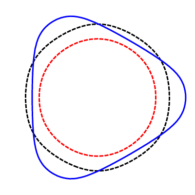
In a one-band model, can be expanded into different angular momentum channels, denoted by the angular momentum quantum number . If the coupling constant in some channel, , is attractive and strong enough to violate the Pomeranchuk condition, , where is the density of states at the Fermi level, then the spherical Fermi surface becomes unstable, leading to a spontaneously distorted Fermi surface as shown in Fig. 1. This is the Pomeranchuk instability. [9] The case of the channel is the electron nematic phase. [18, 7] Similar condensates for other even angular momentum channels can also be (and have been) considered.
In the case of odd angular momentum channels both time reversal and space inversion are spontaneously broken, but the product remains unbroken as these states are not chiral: is unbroken. These states correspond to the type symmetry-breaking states. As can be seen from Figs. 1(b) and (d), the chiral symmetry is preserved and the symmetry can be recovered by space inversion.


IV.2 Two-band model with symmetry
Let us now consider the case of a two-band model. It can be either a system with two bands due to band-structure effects or a bilayer system with a small amount of hybridization (the bonding and antibonding Fermi surfaces are close). We will assume that the system has full translation and rotation symmetries (which will reduce to a point-group symmetry for a lattice system). As before (and for simplicity) we will assume that the system is nonmagnetic (so that the spin degrees of freedom yield only a redundant effect) and that the Fermi surfaces are such that the system is not unstable to the formation of charge density waves or any other instability. We will also ignore possible superconducting states.
We will also assume that the separation between the two bands is small and only the forward-scattering channels need to be considered. Under these approximations, the scattering processes can be classified by their angular momentum channels, as in the case of the one-band model, and we can define bosonic fields (fermion bilinears)
| (16) | |||
| (17) |
Here stands for the normal-order product, relative to the ground state of a Fermi liquid (or gas). Here label the two bands. The matrices are the identity matrix for and the Pauli matrices for , , or . is the polar angle of the momentum vector .
With these definitions, can be written as the sum of all quadratic terms in and that preserve momentum and angular momentum. We further assume that the instability only occurs in one angular momentum channel so that collective excitations in all other angular momentum channels are gapped and irrelevant at low energies. For now, we only consider one particular interaction Hamiltonian of the form
| (18) |
Written in terms of fermionic operators, we can see that this interaction corresponds to the scattering channel . Other scattering channels will be studied later in Sec. IV.4.
In addition to the charge symmetry, this Hamiltonian has an extra internal symmetry corresponding to the relative phase between the two bands. This is because the interaction preserves particle number in each band. This high symmetry requires some amount of fine tuning, but as we will show later, most of the properties are preserved even in the absence of this symmetry (at least perturbatively).
Just as in the case of the one-band model discussed in Sec. IV.1, if an interaction in some angular momentum channel is attractive and in magnitude exceeds a critical value, the ground state of the system becomes unstable. The corresponding order parameters can be taken to be two two-component real vectors in the relative phase manifold
| (19) |
with or . Notice that we use bold characters to represent vectors in space (or momentum space) but use to indicate the two two-component real vector order parameters which form a representation of the nondiagonal piece of group.
In order to preserve the spatial symmetries and the internal symmetry, the Landau free energy has the form
| (20) |
This free energy is very similar to the spin Pomeranchuk instability states in Ref. [8], except that the internal symmetry here is the relative phase instead of the spin . The resulting mean-field phase diagram for the system at hand is shown in Fig. 2.
The coefficients of the free energy can be determined by a mean-field calculation in the same spirit as that of Ref.[8]. We obtain
| (21) | ||||
| (22) | ||||
| (23) |
Here is the energy splitting between the two bands, which is assumed to be much smaller than the Fermi energy , ; is the density of states at the Fermi surface calculated using the average dispersion relation . and are the first- and second-order derivatives of the density of states at the Fermi surface. Higher order terms will be needed for stability reasons if or . For simplicity, we only consider and assume that the higher order term is with .
We will now discuss the structure of the phase diagram of Fig.2. The system has three phases: a) the normal phase with , b) the phase in which , and c) the phase in which they are orthogonal, and . For and , marks the second-order phase boundary between the normal state and either the or the phase, depending on the sign of .
To distinguish this phase with other similar phases which will be discussed below, we indicate this phase as in the phase diagram of Fig. 2 (same with the phase). This phase has a distorted Fermi surface, as shown in Fig. 3(a). In the phase, the Fermi surfaces of both bands are distorted, and their rotational symmetries are reduced from to a -fold discrete symmetry. The phase preserves the symmetry as well as and . A similar phase on the square lattice is discussed in Ref. [19], where it is referred to as the “hidden nematic phase.”

For , the system is in the phase. In this phase, the Fermi surfaces of the two bands remain isotropic with shifted Fermi wave vectors, but the relative phases between the two bands are locked to each other. The relative phase changes by around the Fermi surface, as shown in Fig. 3(b). From a topological point of view, the phase is a map from the Fermi surface to the manifold of the symmetry group. The non-trivial homotopy group of this mapping is described by the Kronecker index, the winding number, which is the angular momentum quantum number . Under the or transformation, the Kronecker index changes sign. Therefore, the phase breaks the and symmetries but preserves their combination. Hence, the phase is a type state and the topological nature of the Kronecker index guarantees that the two degenerate symmetry-breaking ground states of the phase cannot be transformed into each other by any continuous processes.
The line marks the first-order phase boundary between the and phases. When , a first-order phase transition to the phase occurs with decreasing and this first-order phase boundary meets the second-order one at a tricritical point, the black dot in Fig. 2.
IV.3 Hall conductance of the phase
The phase is a type -breaking state with a nonzero spontaneous Hall conductance . As shown in Appendix C, following the results of Haldane,[1] the value of the Hall conductance is quantized for an insulator but not for a conductor such as the phase. However, we can still relate with the Kronecker index of .
Applying Eq. (45), for the phase, the integration region of the integral is the annular region comprised between the two Fermi surfaces of the two bands. If the energy difference between the two bands is small, the component of defined in Eq. (39) of Appendix B can be taken as a constant. Under this approximation, the Hall conductance is
| (24) |
where and can be considered as the and components of a two-dimensional unit vector (by definition, in phase). The integral above is taken around the Fermi surface and measures the Kronecker index of , which counts the number of times the relative phase winds around the Fermi surface. Notice that the prefactor of the integral, is unquantized and can be changed continuously. Hence, as expected, is not quantized in this phase. In particular, vanishes if the Fermi surfaces coincide, .
IV.4 Effects of symmetry-breaking interactions


We now study the effects of interactions that were not considered in Sec. IV.2. The interactions that preserve the particle number in each band, for example, , cannot change qualitatively any conclusions of Sec. IV.2, since these scattering processes preserve the relative symmetry of the two bands. On the other hand, interactions that change the particle number of each band, such as or , break the relative symmetry and potentially can make a difference. However, we can still distinguish the two different ordered phases, and , depending on whether vanishes or not.
To distinguish from the and phases of Sec. IV.2, we refer to the and phases for models with interactions but not interactions as the and states. The corresponding phases when both these two kinds of processes are present will be denoted by and , respectively. The and phases are the most general ones and do not require fine tuning. The main issue we will be interested in is to determine if these are genuinely distinct phases, i.e., if the order parameters have a different behavior in all of these cases.
IV.4.1 and phases
Similar to the phases, the and phases preserve the symmetry. As shown in Figs. 3(c) and 3(e), the Fermi surface of the phase has the same -fold rotational symmetry as , but the phase has a lower, -fold, rotational symmetry. This is because the scattering processes couple the order parameters and to the order parameter of the charge Pomeranchuk instability in each band
| (25) | |||
| (26) |
where is the band index. Hence, and also acquire an expectation value in the phase, which reduces the rotational symmetries from -fold down to -fold. Therefore, for odd, the phase is a type time-reversal symmetry-breaking state.
IV.4.2 and phases
The and phases break both and symmetries but preserve , and hence are type time-reversal symmetry-breaking phases. This conclusion becomes obvious if one notices that the and symmetry breakings in the phases is described by a topological index as shown in Eq. (24). Hence, this property should survive even after adiabatically turning on scattering processes that do not preserve the relative symmetry. However, due to the absence of an exact relative symmetry, the symmetry between and is no longer preserved. As a result, these two order parameters cannot become critical at the same time as one tunes the control parameters. Hence, in order to reach the or phases from the normal Fermi-liquid phase, the system must necessarily either go through a sequence of two phase transitions, at which one order parameter at a time will get a non-zero expectation value, or there will be a direct first-order transition to a state in which both are nonzero. In addition, in the or phases, although the two order parameters and are still perpendicular to each other, without the protection of the relative phase symmetry their magnitudes are no longer equal. Hence, in these phases the Fermi surfaces are no longer isotropic. The phase with angular momentum channel has a Fermi surface with -fold rotation symmetry, as shown in Fig. 3(d). This phase breaks the and symmetries as the phase does but also has Fermi surface with the same -fold rotational symmetry as the and phase. In particularly, in the channel, the phase is a charge nematic state [18, 7] but with broken and symmetry. In the phase, much as in the case of the state, the scattering processes reduce the rotational symmetry to -fold, as shown in Fig. 3(f). Hence, the phase is a charge nematic state with type symmetry breaking.
IV.4.3 Free energy and phase diagram for the and phases
We studied the system without the relative phase symmetry by adding the following interactions
| (27) |
which correspond to the scattering processes. In mean-field theory, the Landau free energy becomes
| (28) |
with and the same as in Eqs. (22) and (23) and
| (29) | ||||
| (30) |
Here . In fact, a complex adds terms such as to the Landau free energy, but upon a suitable rotation, the Landau free energy can be transformed into the form of Eq.(28). The notation is the same as before and the leading higher order term is assumed to be with for simplicity.

The phase diagram is shown in Fig. 4. As predicted by the general symmetry arguments, the phase can be reached through a second-order phase transition at . To reach the phase one must either go through two transitions (using the phase as an intermediate phase) or by a direct first-order transition. The transition between the and phases may be first order or second order depending on details. In this mean-field theory the first-order and second-order phase boundaries meet at a tricritical point (the black dot in Fig. 4) located at and . The first-order phase boundary between and phases meet the second-order phase boundary between and the normal phases, as well as the first-order phase boundary between and the normal phases, at a bicritical point (the circle in Fig. 4).
For most general interactions, the and phases can also occur. The and phases have a similar phase diagram as the and (Fig. 4) and do not exhibit any essentially new phenomena. Hence, we will not present here the mean-field study for the and phases, which has a similar structure to what we have already described in this section.
V lattice models
Most of the conclusions we reached in the continuum models of the previous section can be generalized to the case of lattice models in the absence of degeneracy point. One principal difference in the case of lattice models is that the continuum rotational symmetry is broken down to a discrete point-group symmetry. In particular this gaps out the corresponding Goldstone modes. Another one is that in lattice models the quantum phase transitions to nematic states (and their generalizations) often (although this is not necessarily always the case as there are a few known counterexamples) also involve a topological Lifshitz transition (from closed to open Fermi surfaces) leading to first-order quantum phase transitions.[20, 21]



For one-band models, obviously, the band structure has no degeneracy points. Same as in the continuous model, only the type broken-symmetry state can exist. As an example, we study a one-band model on a simple triangular lattice. This lattice has a -fold rotational symmetry. With properly chosen interactions, the system can undergo a Pomeranchuk instability and form the flux state shown in Fig. 5. In this flux state, three currents flow along the three bonds of the simple triangular lattice. As a result, there is a positive flux in each up-pointing triangle and a negative flux in each down-pointing triangle. The net current and the total flux in each unit cell are both zero, but the rotational symmetry of the Fermi surface will in general be reduced from -fold to -fold symmetry, except when the flux in each triangle is for integer . This is so because a gauge transformation can change the flux in a triangle by and similar effects is known to occur for the square lattice. [3] The same analysis with very little modification applies to the “Varma loop model” (Ref. [14]) and to a model on the square lattice with effective diagonal hopping terms and the same pattern of time-reversal symmetry breaking recently discussed in Ref. 22 which are also type time-reversal symmetry-breaking states. When the flux is not , , where is the identity operator. As shown in Fig. 5, the Fermi surface of a state with flux different from has -fold rotational symmetry, which corresponds to the Pomeranchuk instability, and this state belongs to the type symmetry-breaking states.


In two-band lattice models without degeneracy points, and phases can also occur much as in the continuum model discussed before. The simplest example is a bilayer model in which two layers of a lattice system are separated by a small distance. If the separation is small enough, three dimensional (3D) effects can be ignored. For a bilayer model, two bands (bonding and antibonding) can be formed and they usually have no degeneracy. In Ref. [19], Puetter, Doh, and Kee studied a system of this type and found a “hidden nematic phase” on a bilayer square lattice, which is one of the example of the phase.
For band structures with degeneracy points, the type phase just requires one order parameter quadratic in fermions. A well-known example is the flux states in the honeycomb lattice. The band structure of the honeycomb lattice has two degeneracy points (the Dirac nodal points) at the two corners of its first Brillouin zone. As shown in Appendix B and Fig. 6, there is a “monopole flux” passing through each Dirac point. If the two Dirac points get masses with the same sign, they cannot cancel each other; the and symmetries are broken, as shown in Fig. 1 of Ref. [23]. (A similar effect is found in the mean-field theory of the chiral spin liquid [3, 17].) A recent mean-field study of a system of interacting fermions on the honeycomb lattice (at half filling) shows that this state can be stabilized by repulsive next-nearest-neighbor interactions. [24]
Another example is a fermionic system on the crossed-chain lattice as shown in Fig. 7. This lattice has two sublattices.[25] The tight-binding model on this lattice has two bands and one degeneracy point in each Brillouin zone where the two bands touch. This degeneracy point has monopole flux [Fig. 6]. If the four-fold rotation symmetry of the lattice is broken explicitly upon the introduction of a different chemical potential for each sublattice, or spontaneously via a (quantum nematic) symmetry breaking, the degeneracy point with flux splits into two Dirac points, each with flux . Similar as in the case of the honeycomb lattice, a Dirac mass term which removes the band crossing breaks the and symmetries. This state corresponds to the flux state shown in Fig. 7 with order parameter
| (31) |
where , , , and are the creation and annihilation operators for the two sublattices of the crossed-chain lattice at momentum . It can be shown that this is a type time-reversal symmetry-breaking state which can be stabilized by an arbitrarily weak nearest-neighbor repulsive interaction for some range of hopping amplitudes and electron densities.[27] Recently, Ran and coworkers [28], found similar degeneracy points with monopole flux in FeAs-based materials with symmetry. Hence, similar symmetry-breaking phases may be possible in such systems as well.
The state shown in Fig. 7 has a close analogy to the DW state with symmetry [Fig. 2.(c) in Ref. [29] and Fig. 1 in Ref. [30]]. Both phases are type II symmetry-breaking states. They have similar order parameters but with very different physical origins. First of all, the lattice structure of our model is a crossed-chain lattice while the DW state is defined on a simple square lattice. Hence, the alternating of the diagonal hopping strength (the crosses) in our model is due to a lattice effect (an explicit symmetry breaking), while in DW state it is due to spontaneous translational-symmetry breaking. Secondly, due to the special lattice structure of the crossed-chain lattice, a non-generic (non-Dirac) band crossing is presented at momentum in the absence of interactions. This band touching leads to an infinitesimal instability to the symmetry-breaking flux state shown in Fig. 7, where the DW state requires a finite interaction to be reached.
We end the discussion on lattice models with a few remarks on the Emery model, which describes the plane of cuprates. The Varma loop state, shown in Fig. 7, is a type state that breaks the and but not the and .[31] Without breaking translational and charge symmetries, we show in Figs. 7 and 7 two other nonmagnetic states that break the symmetry as well as . The state shown in Fig. 7 is the same as the state in Fig. 7, if we notice that the oxygens ( and orbitals) in the Emery model form a crossed-chain lattice (rotated by ). The state in Fig. 7 involves three bands and there is a flux piercing each small triangle formed by neighboring , , and orbitals. In each unit cell, three of the triangles have flux but the fourth triangle has flux , with zero total flux in the unit cell. In this state all the , and symmetries are broken (and none of the pairs , , or is preserved) while remains unbroken. Hence, this state is a mixture of states of type and time-reversal symmetry breaking.
VI symmetries and finite temperature transitions
For a two-band model for a system in the continuum (i.e., ignoring the explicit breaking of rotational symmetry by the underlying lattice), the and phases break spontaneously two continuous symmetries: the rotational invariance and the relative phase symmetry. Hence, two Goldstone modes are generated in the broken-symmetry phase. At finite temperatures, the thermal fluctuations of these two Goldstone modes destroy this long-range order. The thermodynamic phase transition is in the universality class of a system of two models which will undergo a Kosterlitz-Thouless type phase transition.
For the case of the and phases, the relative phase symmetry of the bands is broken explicitly by the effects of the interactions, which do not preserve particle number on each band as a good quantum number. Hence, only one continuous symmetry, , remains and it is broken spontaneously in this phase at . Since this is a continuous symmetry, the finite temperature transition between the normal state and the or the phase also belongs to the Kosterlitz-Thouless (KT) universality class, in this case with a single order-parameter field.
The direct transition from the normal state to the or states was shown in Sec. IV.4 to be first order at zero temperature. Therefore one expects this transition to remain first order even at finite temperature up to a critical value where the phase boundary reaches a tricritical (or multicritical) point. In general, for a system with full rotational invariance , the transition from these phases to the normal state should be in the KT universality class as well.
For lattice systems, rotational symmetry is broken down to a discrete subgroup, the point-group symmetry of the underlying lattice. Hence the only continuous symmetry left to be spontaneously broken in the and phases is the relative phase. Thus, the finite temperature transitions from the and phases to the normal state are also KT transitions. For lattice systems in which the , and , phases can be realized there are no continuous symmetries present since the relative symmetry is broken by the interactions. Hence, in general the thermodynamic transitions from the and phases to the normal state only involve the restoration of time-reversal invariance and the discrete point-group symmetries broken in these low-temperature phases (up to important caveats discussed below).
For a lattice system, except for the and phases, whose existence is not generic and requires fine tuning, the and phases only break discrete symmetries and hence do not have Goldstone modes in their excitation spectra. As a result, the fermionic quasiparticles are the only low-energy excitations in these broken-symmetry phases. This implies that the Fermi-liquid picture should remain valid in these low-temperature phases even if the fluctuations are stronger than what is allowed in a naive mean-field treatment.


We will now give a more careful analysis of the nature of the thermal phase transitions for the , , , and phases in lattice, which have richer structures, based on an analysis of the symmetry.
Let us begin by discussing the d-wave type phase in a square lattice. In this case, in addition to the time-reversal symmetry, this phase also lowers the invariance under spatial rotation to rotation (2D space inversion), which is also a symmetry breaking. Formally, the phase has a broken symmetry. In the case of the phase, the situation is similar except that the time-reversal even symmetry requires a different physical interpretation (see Appendix D).
From this view point the natural description of the thermal phase transitions out of the or phase should be in the 2D Ashkin-Teller universality class. In what follows we will consider the conceptually more straightforward phase, but the same analysis also applies to the more intricate phase.
If the low-temperature phase is the phase diagram can have the general topology of the one shown in Fig. 8. As temperature is raised it may undergo a direct phase transition to the normal phase or have two thermal transitions. In the latter case, the intermediate phase arises from the restoration of one of the symmetries, either time reversal or spatial rotations. Thus the intermediate temperature phase is either a time-reversal even nematic phase (the phase) or a spatially isotropic phase with broken time-reversal invariance. In any case, the transition between these two states in two space dimensions is continuous and in the 2D Ising universality class. One should note that it is possible to conceive the existence of a spatially isotropic intermediate phase with broken time-reversal symmetry even at . However a state like that cannot be reached within mean-field theory as it results from the “quantum melting” of one of the states of the phase.
These arguments suggest that the finite temperature critical behavior of this system is in general describable by a 2D classical Ashkin-Teller model, as far as the thermal transitions are concerned. Indeed this would be the case if the two Ising transitions were to meet at a multicritical point, which would necessarily be in the 2D four-state Potts model universality class, a KT transition. If this scenario is correct, the transition from the phase to the normal state should have a line of continuous transitions with varying exponents. Since the quantum phase transition (at ) between the normal state and the phase is first order, this scenario requires the existence of a tricritical point at some intermediate but low temperature. A similar phase diagram was found in interacting monomer-dimer models on a 2D square lattice.[32]
An alternative possible scenario is that the two Ising transitions do not meet at a multicritical point. Instead, that the lower temperature Ising transition becomes first order at some value of the control parameter, i.e., a 2D Ising tricritical point. The general topology of the phase diagram is depicted in Fig.8. Here too the intermediate phase can either be an phase, in which case time reversal is restored at the lower temperature transition and the intermediate phase is nematic, or isotropy is restored first and the intermediate phase breaks time-reversal.
Still a third possibility arises if at the and normal phases are separated by a region of the phase. In this case the transition is continuous, and one would generally expect two thermal transitions, as shown in Fig.8, with an intermediate temperature phase that at least at low temperatures must be an phase. The possibility of another intermediate phase discussed above, isotropic and breaking, cannot be excluded even in this scenario.
Finally, let us consider briefly the case of lattice symmetry breaking, beyond the symmetry of the square lattice we have been discussing here, i.e., simple triangular and honeycomb lattices. We will now have to consider more general angular momentum channels, with even or odd. Specifically, for the simple triangular and honeycomb lattices the simplest cases of interest have and broken by the symmetry. An example of this is the one-band model on a simple triangular lattice discussed above.
Two-band models on these lattices allow for a richer structure. The simplest case is a state with an particle-hole condensate without relative particle-number conservation of any type. This state breaks spontaneously the inversion symmetry and the chiral symmetry. Hence, the thermal transitions to the normal state of this phase also have a , as in the square lattice case discussed above, with a phase diagram similar to those in Figs.8-8. (Just as in the case of the square lattice, this analysis also applies to the phase with the same caveats on the interpretation of the symmetries.)
A different symmetry-breaking pattern arises on both the simple triangular and honeycomb lattices if the condensate is in the particle-hole channel. In the state with , the symmetry is lowered to (inversion in 2D) symmetry, where the axis is lifted. Hence, is the broken rotational symmetry manifold of the order parameter. In addition to this , this phase also breaks the time-reversal symmetry, which here is equivalent to chiral symmetry. Hence, it breaks a symmetry. The thermal phase diagram for this problem is more complex (and old problem) than the cases we presented above (see Refs.[33] and [34] and references therein). The structure of the phase diagram can be summarized in three cases: a) a direct transition to the normal state, b) an intermediate temperature critical phase, and c) an intermediate phase with long-range order. In the first case, the transition between the phase and the normal phase is a direct first-order transition (similar to that of the closely related six-state Potts model). In the second case, there is a finite range of temperatures in which the system is critical, as in the model, and has two KT-type transitions at each end-point. The third case consists of a sequence of partial restorations of the and broken symmetries of the state through intermediate temperature phases with either nematic order and no broken time-reversal symmetry or with broken time-reversal invariance and full isotropy.
VII Discussion
We studied microscopic fermionic models (generally in metallic phases) with spontaneous breaking of time-reversal invariance. We considered one-band models and two-band models (ignoring spin) with and without separate conservation of particle number in each band. The time-reversal breaking phases can be classified in two classes:
- 1.
Type phases, which break time reversal () and space inversion () but do not break chirality (). We found that type phases occur in both one-band and multiple-band fermionic systems in a generalized nematic ground state with a (particle-hole) condensate in an odd angular momentum channel. Examples of type phases we discuss are one-band nematics with and two-band models in the state, which has a particle-hole condensate with odd without independent particle number conservation in each band.
- 2.
Type phases, which break time reversal () and chirality () but do not break space inversion (). Type phases have a spontaneous (non-quantized) anomalous Hall effect. We found that type phases are not realized in one-band models. In two (and multiple) band models they occur in interband particle-hole condensates with even angular momentum if particle number is not separately conserved in each band ( phases), [35] and in any angular momentum channel provided particle number is either preserved in each band ( phases) or conserved modulo ( phases).
Each class of states has unique experimental signatures that can be detected in linear and nonlinear conductivity measurements, and in the optical response with polarized light.
Let us discuss first how these phases can be detected in transport. It is well known that electronic nematic phases induce an anisotropy in the conductivity tensor.[36, 37, 38, 18, 7, 39] In a metallic system, an in-plane electric field induces a current which can be expanded as a power series in the electric field ,
| (32) |
with , , and being or . The first term in Eq.(32) is the linear response, and the second term is the leading nonlinear response. The different components of the conductivity tensor (and of the nonlinear response) can be arranged to transform properly under chiral and space inversion symmetries, and can be used to detect these broken-symmetry phases in experiment. Thus, the conductivity tensor is sensitive to both rotations under and chirality, while the third rank nonlinear conductivity tensor is odd under inversion. To detect systems with condensates with , it is necessary to consider higher order nonlinear response terms. Thus, one can construct phenomenological “order parameters” using the electrical response tensors, and the simplest ones are presented in Table 1.
The signatures of type breaking phases can be detected through nonlinear optical processes, such as polarized Raman scattering. [They can also be checked directly by angle-resolved photoemission spectroscopy (ARPES) by detecting the anisotropy of the Fermi surface.] On the other hand, type phases, such as the phases, can be detected optically through a nonzero Kerr effect (in the absence of external magnetic fields).
| Normal phase | zero | zero | zero |
|---|---|---|---|
| Nematic ( phases) | nonzero | zero | zero |
| Type ( phases, and odd) | zero or nonzero | zero | nonzero |
| Type (, phases, and odd) | zero or nonzero | nonzero | zero |
The problem of constructing phases of electronic systems with broken time-reversal invariance was presented here mainly from its intrinsic conceptual interest. Our interest in this problem has been to a large extent motivated by the recent discovery of time-reversal symmetry-breaking effects in the ruthenates and in the cuprates. We should stress that although the theory we presented in this paper as it stand cannot describe a strongly correlated system, the patterns of symmetry breaking, as well as their consequences, should be of more general validity. The strongest experimental evidence available to date of time-reversal symmetry breaking in superconductors is in the layered compound Sr2RuO4. Kerr effect rotation experiments[40] and corner junction experiments[41] strongly suggest that this material may indeed have a -wave superconducting state which breaks spontaneously time-reversal symmetry. This is consistent with a theoretical prediction[42] of a condensate with a order-parameter symmetry. This evidence is however not fully uncontroversial given the conflicting experimental results of Ref.[43] which, so far, have failed to detect the expected edge currents of the superconductor. Recent high-precision Kerr rotation experiments[44] have now given evidence of weak but detectable time-reversal symmetry breaking in the underdoped pseudogap regime of the high compound YBa2Cu3O6+y. Neutron-scattering experiments in underdoped YBa2Cu3O6+y [45, 46], and in HgBa2CuO4+d [47] similarly suggest that the breaking of time-reversal invariance may also occur in these materials. These recent discoveries in the cuprates and in Sr2RuO4 have renewed interest in the possible mechanisms of time-reversal symmetry breaking in strongly correlated systems. However, it is worth to note that, in addition to the noted evidence of time-reversal symmetry breaking, neutron-scattering experiments[48] and transport experiments[37] find strong evidence for nematic charge order in YBa2Cu3O6+y in the same doping range. It is unreasonable to believe that these two phases can be unrelated to each other, and perhaps they have a common origin. In this sense, the phases found in this paper may shed some light on these issues.
One important problem that we have not discussed in this work is the role of disorder in these phases. It is well known that disorder couples as a random field to the order parameter of anisotropic nematic-like phases,[49, 39] destroying the ordered state and rendering the system glassy. The same applies to other phases we discussed here that break spontaneously either point-group symmetries and/or inversion. On its own, nonmagnetic disorder cannot couple directly to the chiral symmetry and does not destroy automatically a type time-reversal breaking state. However, if the spin degrees of freedom are also included even nonmagnetic disorder can couple indirectly to time-reversal breaking order parameters through the effects of spin-orbit interactions. In this case the system becomes a -breaking glassy state. On the other hand, disorder can induce and breaking effects in phases such as type states by breaking locally translation, inversion, and point-group symmetries of the system. In any case, the time-reversal symmetry-breaking effects induced by disorder should be quite weak.[44]
Other states that break time-reversal symmetry to varying degrees have been postulated in the context of high compounds. These states assume the existence of spontaneously circulating currents in the ground state. They include the loop state advocated by Varma, [50, 14] which breaks time reversal but not translation invariance, and the -density wave state of Charkravarty, Laughlin, Morr and Nayak [51, 29], a DW state that breaks time reversal and translation invariance (by one lattice spacing) but it is invariant under the simultaneous action of both transformations. In the absence of disorder neither of these states exhibits a uniform Kerr effect. Tewari et al[30] proposed a DW state with symmetry that breaks translational symmetry and has nonzero Kerr effect.
There is a close analogy between the phase and the (or ) superconducting state. They both need two real order parameters that couples the rotational symmetry and an internal symmetry to break the and symmetries. The symmetry in the spin triplet condensate in the particle-particle channel in superconductors is the charge (“gauge”) symmetry, which is an exact symmetry of the system and cannot be broken explicitly. On the other hand, the formally analogous phase is a particle-hole condensate which breaks spontaneously the relative phase symmetry of a multiband system. This symmetry in general is not exact but it is asymptotically exact “emergent” symmetry at the Fermi-liquid fixed point, since the symmetry-breaking terms are formally irrelevant (“dangerous irrelevant”) operators which are always present in any real system. The difference, between exact and “emergent” symmetries, has a direct consequence on the structure of the phase diagram, rendering the quantum phase transition from the normal state to the phase first order or through an intermediate phase.
Our phases have a close similarity with the phases (with the same name!) in spin-1/2 fermionic systems with anisotropic phases such as those discussed in Refs. [10] and [8]. However, the phases of those systems are not type symmetry-breaking states for two reasons. First under time reversal all three components of the spin polarization of the quasiparticles changes sign. In contrast, here we have used the Pauli matrices to act on an internal space unrelated with the electron spin, a “pseudospin” representing the multiple electronic bands. In our case only the complex, , component is odd under time reversal. Secondly, the internal symmetry in our problem is only an approximate phase symmetry, while in the spin problem it is the full group (in the absence of the spin-orbit couplings). We have shown that for systems with degenerate bands, the (natural) symmetry is ( for this case), and the Berry connection , defined in Sec. II, is always trivial and it can always be eliminated by a gauge transformation (it is a gauge transformation!) due to Eq. (33). Hence, the actual Berry phase [no matter or ] is zero if the symmetry is exact. As a result, in the fully symmetric case (as well as in the spin-1/2 model) there are no type symmetry-breaking states. This can also be seen if we notice that the map from the Fermi surface to the internal group is , which has a nontrivial homotopy group, , with a non-vanishing Kronecker index. In contrast, for the case of spin-1/2 systems, the mapping has a trivial homotopy, , and does not have a nontrivial topological index. We should emphasize that the electronic quasiparticles of the systems we have considered do carry spin-1/2, but these degrees of freedom play no role in the phases we have discussed as they are paramagnetic.
Acknowledgements.
We thank Steven Kivelson and Congjun Wu for many insightful discussions. This work was supported in part by the National Science Foundation grant DMR 0758462 at the University of Illinois (EF) and by the Department of Energy, Division of Basic Energy Sciences under Award DE-FG02-07ER46453 through the Frederick Seitz Materials Research Laboratory at UIUC (KS and EF).Appendix A two-band models
By definition, the matrix satisfies
| (33) |
This constraint on implies that the off-diagonal terms and the diagonal terms are related. It follows that
| (34) |
which leads to the conclusion that there is no Berry phase in the overall (charge) sector.
For a two-band model, we can construct three gauge invariant objects that are sensitive to time-reversal symmetry breaking
| (35) | |||
| (36) | |||
| (37) |
However, due to Eq. (33), only one of them is linearly independent.
Hence, in the study of the symmetry breaking in any two-band model, only the diagonal term (or ) is needed to be considered. The same conclusion is trivially valid for one-band models.
Appendix B the topological and physical meaning of Wilson loops
From a topological point of view, in a two-band model, a unitary transformation at momentum belongs to the group . By removing the gauge degrees of freedom, the physical degrees of freedom are in the manifold . Hence, for each closed loop in momentum space, a map can be defined. Similar to the coherent-state path integral of spin (see for instance Ref. [17]), this map leads to a Wess-Zumino term. We will show here the Berry phase studied in the main text is half of the Wess-Zumino term of this map (mod ).
For a two-band model, the kinetic energy part of the Hamiltonian is a Hermitian matrix, which can be expanded in the basis of the identity matrix and the three Pauli matrices:
| (38) |
Away from degeneracy points, is nonzero. Hence, we can define a 3D unit vector
| (39) |
From a topological point of view, this 3D unit vector field is a map from the momentum space (with degeneracy points removed) to .
If we define the polar coordinates of the unit vector as and , where , the Hamiltonian can be diagonalized by a unitary transformation, , where
Here and is any function of the momentum, which reflects the gauge freedom in a two-band model. Therefore, we get
| (42) |
The loop integral around contour is
| (43) |
where is an integer measuring the winding number of the angle . By comparison, the Wess-Zumino term of the map from to is
| (44) |
Here is an arbitrary 2D manifold whose boundary is and is an integer determined by the choice of . Hence, we conclude that the Berry phase is half of the Wess-Zumino term up to .
Under a change in chirality, the Wess-Zumino term changes sign (mod ). Therefore, changes into under , which is the same as . Hence, is invariant under .
Appendix C Hall conductance
For the Hamiltonian shown in Eq. (38), the Hall conductance can be evaluated as in Ref. [52], using the three-component unit vectors defined in Eq. (39),
| (45) |
Here the integration region is the area in momentum space where one band is filled and the other is empty.
For insulators, the region is the whole momentum space (the first Brillouin zone for lattice models), which is a compact manifold. Hence, is the Kronecker index of the mapping from a compact manifold to , the first Chern number, which is quantized to be an integer. It measures how many times the compact manifold wraps around the sphere . For conductors, the boundary of is the Fermi surface, which implies that is not a compact manifold. Hence, for conductors in general is not quantized.[1]
Using the conclusion from Appendix B, the Hall conductance can be related to the loop integral as
| (46) |
where the contour is the boundary of , which is the Fermi surface, and we choose the gauge where is analytic in region to remove the uncertainty in . This result is straightforward if we notice that contains all the information of and symmetry breaking in two-band models. Therefore, , which measures the type symmetry breaking at low energies, must be directly related with , where is the Fermi surface, which dominates the low-energy physics.
Appendix D Symmetry analysis of the and phases
For a -wave-like () phase on a square lattice, the symmetry breaking is reduced from to . In the normal phase, in addition to the point-group symmetry of the square lattice , there is a internal symmetry corresponding to the relative phase shift by between the two bands of a system, in which the relative particle number is conserved mod , and the relative phase symmetry is thus reduced to phase shifts of the electron wave functions between the two bands by , and . In the phase, the order parameter is blind under the simultaneous action of a spatial rotation and the relative phase shift by . Hence, the resulting symmetry of the ordered phase is . Therefore, the thermal phase transition from the state to the normal state is in the 2D Ising universality class. The same analysis applies to the phase, except that the broken symmetry are simply , which only involves the spatial symmetry.
For the phase, in addition to the symmetry breaking just discussed above, an additional time-reversal symmetry is broken. Hence, the phase has a broken symmetry.
References
- [1] F. D. M. Haldane, Phys. Rev. Lett. 93, 206602 (2004).
- [2] V. Kalmeyer and R. B. Laughlin, Phys. Rev. Lett. 59, 2095 (1987).
- [3] X.-G. Wen, F. Wilczek, and A. Zee, Phys. Rev. B 39, 11413 (1989).
- [4] R. B. Laughlin, Phys. Rev. Lett. 60, 2677 (1988).
- [5] A. L. Fetter, C. B. Hanna, and R. B. Laughlin, Phys. Rev. B 39, 9679 (1989).
- [6] M. V. Berry, Proc. Roy. Soc. Lond. A392, 45 (1984).
- [7] V. Oganesyan, S. A. Kivelson, and E. Fradkin, Phys. Rev. B 64, 195109 (2001).
- [8] C. Wu, K. Sun, E. Fradkin, and S.-C. Zhang, Phys. Rev. B 75, 115103 (2007).
- [9] I. I. Pomeranchuk, Sov. Phys. JETP 8, 361 (1959).
- [10] C. Wu and S.-C. Zhang, Phys. Rev. Lett. 93, 036403 (2004).
- [11] R. Shankar, Rev. Mod. Phys. 66, 129 (1994).
- [12] E. I. Blount, in Solid State Physics, edited by F. Seitz and D. Turnbull (Academic, New York, 1962), vol. 13.
- [13] G. Sundaram and Q. Niu, Phys. Rev. B 59, 14915 (1999).
- [14] C. M. Varma, Phys. Rev. B 73, 155113 (2006).
- [15] M. Kohmoto, Ann. Phys. (N. Y.) 160, 343 (1985).
- [16] J. E. Avron, R. Seiler, and B. Simon, Phys. Rev. Lett. 51, 51 (1983).
- [17] E. Fradkin, Field Theories of Condensed Matter Systems (Addison-Wesley, Redwood City, CA, 1991).
- [18] S. A. Kivelson, E. Fradkin, and V. J. Emery, Nature 393, 550 (1998).
- [19] C. M. Puetter, H. Doh, and H.-Y. Kee, Phys. Rev. B 76, 235112 (2007).
- [20] I. Khavkine, C.-H. Chung, V. Oganesyan, and H.-Y. Kee, Phys. Rev. B 70, 155110 (2004).
- [21] H. Yamase, V. Oganesyan, and W. Metzner, Phys. Rev. B 72, 035114 (2005).
- [22] E. Berg, C. C. Chen, and S. A. Kivelson, Phys. Rev. Lett. 100, 027003 (2008).
- [23] F. D. M. Haldane, Phys. Rev. Lett. 61, 2015 (1988).
- [24] S. Raghu, X.-L. Qi, C. Honerkamp, and S.-C. Zhang, Phys. Rev. Lett. 100, 156401 (2008).
- [25] An effective model with this geometry can be shown to arise in the strong-coupling regime of the Emery model of the cuprates.[26, 27].
- [26] S. A. Kivelson, E. Fradkin, and T. H. Geballe, Phys. Rev. B 69, 144505 (2004).
- [27] K. Sun (2008), unpublished.
- [28] Y. Ran, F. Wang, H. Zhai, A. Vishwanath, and D.-H. Lee (2008), unpublished, eprint arXiv.org:0805.3535.
- [29] C. Nayak, Phys. Rev. B 62, 4880 (2000).
- [30] S. Tewari, C. Zhang, V. M. Yakovenko, and S. Das Sarma, Phys. Rev. Lett. 100, 217004 (2008).
- [31] As noted in Sec. II, Varma’s loop state breaks time reversal but it does not have Berry phases. Hence this breaking state is neither type nor type and it does not have a spontaneous anomalous Hall effect.
- [32] S. Papanikolaou, E. Luijten, and E. Fradkin, Phys. Rev. B 76, 134514 (2007).
- [33] J. L. Cardy, J. Phys. A.: Math. Gen. 13, 1507 (1980).
- [34] F. C. Alcaraz and R. Köberle, J. Phys. A.: Math. Gen. 13, L153 (1980).
- [35] The phase in an odd angular momentum channel is a type I-type II mixed state.
- [36] M. P. Lilly, K. B. Cooper, J. P. Eisenstein, L. N. Pfeiffer, and K. W. West, Phys. Rev. Lett. 82, 394 (1999).
- [37] Y. Ando, K. Segawa, S. Komiya, and A. N. Lavrov, Phys. Rev. Lett. 88, 137005 (2002).
- [38] R. A. Borzi, S. A. Grigera, J. Farrell, R. S. Perry, S. J. S. Lister, S. L. Lee, D. A. Tennant, Y. Maeno, and A. P. Mackenzie, Science 315, 214 (2007).
- [39] S. A. Kivelson, E. Fradkin, V. Oganesyan, I. Bindloss, J. Tranquada, A. Kapitulnik, and C. Howald, Rev. Mod. Phys. 75, 1201 (2003).
- [40] J. Xia, Y. Maeno, P. T. Beyersdorf, M. M. Fejer, and A. Kapitulnik, Phys. Rev. Lett. 97, 167002 (2006).
- [41] F. Kidwingira, J. D. Strand, D. J. V. Harlingen, and Y. Maeno, Science 314, 1267 (2006).
- [42] T. M. Rice and M. Sigrist, J. Phys.: Condens. Matter 7, L643 (1995).
- [43] J. R. Kirtley, C. Kallin, C. W. Hicks, E. A. Kim, Y. Liu, K. A. Moler, Y. Maeno, and K. D. Nelson, Phys. Rev. B 76, 014526 (2007).
- [44] J. Xia, E. Schemm, G. Deutscher, S. A. Kivelson, D. A. Bonn, W. N. Hardy, R. Liang, W. Siemons, G. Koster, M. M. Fejer, and A. Kapitulnik, Phys. Rev. Lett. 100, 127002 (2008).
- [45] B. Fauqué, Y. Sidis, V. Hinkov, S. Pailhès, C. T. Lin, X. Chaud, and P. Bourges, Phys. Rev. Lett. 96, 197001 (2006).
- [46] H. A. Mook, Y. Sidis, B. Fauqué, V. Balédent, and P. Bourges, Phys. Rev. B 78, 020506(R) (2008).
- [47] Y. Li, V. Balédent, N. Barisic, Y. Cho, B. Fauqué, Y. Sidis, G. Yu, X. Zhao, P. Bourges, and M. Greven (2008), unpublished, eprint arXiv:0805.2959.
- [48] V. Hinkov, D. Haug, B. Fauqué, P. Bourges, Y. Sidis, A. Ivanov, C. Bernhard, C. T. Lin, and B. Keimer, Science 319, 597 (2008).
- [49] E. W. Carlson, K. A. Dahmen, E. Fradkin, and S. A. Kivelson, Phys. Rev. Lett. 96, 097003 (2006).
- [50] C. M. Varma, Phys. Rev. B 55, 14554 (1997).
- [51] S. Chakravarty, R. B. Laughlin, D. K. Morr, and C. Nayak, Phys. Rev. B 63, 094503 (2001).
- [52] V. M. Yakovenko, Phys. Rev. Lett. 65, 251 (1990).