New Calculations of Stellar Wind Torques
Abstract
Using numerical simulations of magnetized stellar winds, we carry out a parameter study to find the dependence of the stellar wind torque on observable parameters. We find that the power-law dependencies of the torque on parameters is significantly different than what has been used in all spin evolution models to date.
Keywords:
MHD—stars: magnetic fields—stars: rotation—stars: winds, outflowsClassification:
95.30.Qd, 97.10.Kc, 97.10.Me, 97.20.Jg1 Introduction
Studying rotation gives us a better understanding of how stars form, how they function, how they evolve, and how they interact with their environment. To understand the rotation rates and rotational evolution of cool stars, we must understand how they lose angular momentum. We know that stellar winds are of primary importance for this, but the existing analytic theory for calculating the stellar wind torque has not substantially changed in 20 years. Since that time, numerical simulations have revealed that a number of the underlying assumptions of this theory are not generally valid and that a new formula for the torque is needed.
Numerical simulations have the advantage that they typically require fewer assumptions (and often fewer tunable parameters) than analytic theory. However, the disadvantage is that a single simulation does not give much insight into how the physics depends upon the parameters. To improve this situation, Matt and Pudritz (2008) carried out a small simulation parameter study, using ideal magnetohydrodynamic simulations to compute axisymmetric, steady-state solutions of Solar-like winds from magnetized stars. That work focused on accretion-powered winds from pre-main-sequence stars, and the reader will find all details in that paper. Here, we summarize the results and rescale the physical parameters and results of those simulations to be in a regime more representative of Solar-like main sequence stars.
2 Wind Simulation Method and Results
The parameters and values adopted for the fiducial wind are listed in table 1. The parameters are the stellar mass (), radius (), dipole magnetic field strength at the equator (), wind mass outflow rate (), wind thermal sound speed divided by the surface escape speed (), the adiabatic index (, where ), and the spin rate expressed as a fraction of breakup speed, , where is the angular spin rate of the star and is Newton’s gravitational constant.
| Parameter | Value |
|---|---|
| 1.0 | |
| 1.0 | |
| (dipole) | 10 Gauss |
| /yr | |
| 0.1 | |
| 0.222 | |
| 1.05 |
In the simulations, the wind solution is completely determined by the boundary conditions applied at the surface of the star. At that boundary, the magnetic field is anchored into the star, which is assumed to be rotating as a solid body. The field geometry is a dipole at the stellar surface (except for two cases with a quadrupolar field). The surface temperature and density is uniform and held fixed throughout the simulation. The wind velocity is determined dynamically by the simulations.
We ran the fiducial case and 16 other cases, listed in table 2. In each case, we changed only one parameter value relative to the fiducial case. The changed parameter and its value is listed in the first column of table 2.
| Case | () | ( ) | |
|---|---|---|---|
| fiducial | 5.91 | 5.53 | 6.97 |
| = 0.004 | 5.81 | 0.304 | 8.33 |
| = 0.2 | 5.84 | 8.81 | 6.26 |
| = 0.05 | 5.88 | 3.31 | 7.65 |
| = 20 G | 5.81 | 10.2 | 9.55 |
| = 100 G | 6.00 | 43.1 | 19.3 |
| 50 G quadrupole | 5.84 | 4.28 | 6.17 |
| 100 G quadrupole | 6.03 | 2.11 | 7.53 |
| low | 0.584 | 1.56 | 11.8 |
| very low | 0.118 | 0.638 | 16.7 |
| = 0.75 | 5.81 | 3.44 | 5.96 |
| = 1.5 | 5.91 | 10.7 | 8.75 |
| = 0.5 | 5.97 | 4.59 | 7.52 |
| = 2 | 5.88 | 6.59 | 6.42 |
| = 0.245 | 5.84 | 4.97 | 6.64 |
| = 0.192 | 5.91 | 5.97 | 7.23 |
| = 1.10 | 5.84 | 6.84 | 7.79 |
The simulations result in a Parker-like, thermally driven wind that is modified, self-consistently, by the stellar rotation, presence of the magnetic field, and polytropic equation of state. Thus, the total mass loss rate in the flow, listed in table 2, is not a true parameter but is actually a result of the simulation. In order to treat as a pseudo-parameter, our method is to iteratively change the value of the density at the stellar surface until the desired value of is obtained, within a tolerance of a few percent.
After each simulation reaches a steady-state solution, we calculate the total angular momentum loss rate, , by integrating the angular momentum flux over a surface enclosing the star. Then we use the formula
| (1) |
from analytic theory, to calculate the value of , the “magnetic lever arm” length. Since the winds are multi-dimensional, represents the mass-loss-weighted average of the Alfvén radius in the flow. Table 2 lists the results for each case.
3 Toward a Predictive Torque Theory
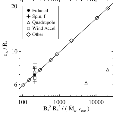
Analytic theory suggests that the dimensionless combination of parameters is of fundamental importance for determining the wind physics. We plot as a function of this parameter combination in figure 1. Using a simple power law formulation,
| (2) |
we find that and provides an excellent fit to the fiducial case and the simulations with variations in , , , or .
The combination of equations (1) and (2) gives
| (3) |
This is essentially the same formula as derived by Kawaler (1988). However, without the aid of numerical simulations, Kawaler had to parameterize the magnetic field structure in the wind and make assumptions about how the wind velocity depends on parameters. Thus, he preferred a value of , which is significantly different than the value obtained by our simulations. The value obtained by simulations should be viewed as more accurate, since the simulations self-consistently calculate the field structure and wind velocity in multiple dimensions and thus have fewer parameters and assumptions.
Finally, it is important to point out that neither the work presented here nor any previous analytic theory has properly determined the dependence of the torque on the spin rate or wind driving parameters. This is evident in figure 1, since the fit of equation (2) is less precise for cases with different spin rates () or wind acceleration parameters ( or ). Also, it is clear from the outlying triangles in the figure that the torque is very sensitive to field geometry. Due to the limited number of simulations in this study with changes in the spin rate, wind driving, and field geometry, it is still not clear what is the appropriate functional form for the dependence of on these parameters. Future work will include a larger parameter study, with the goal of determining the precise dependence on all relevant parameters.
This work has implications for understanding the observations of stellar rotation at all evolutionary phases, as well as the emperically established method of gyrochronology (Barnes, 2003). As an illustrative example of how the new power law index changes our understanding, consider that the empirical Skumanich (1972) relationship for the spin-down of main-sequence stars suggests . Under the assumption that in equation (3), a particular dynamo relationship, where , elegantly explains the Skumanich relationship. However, we showed that is instead much closer to 0.2. This suggests, e.g., either that a different dynamo relationship is appropriate or that the mass loss rate depends in a particular way on the stellar rotation rate.
References
- Matt and Pudritz (2008) S. Matt, and R. E. Pudritz, ApJ 678, 1109–1118 (2008), arXiv:0801.0436.
- Kawaler (1988) S. D. Kawaler, ApJ 333, 236–247 (1988).
- Barnes (2003) S. A. Barnes, ApJ 586, 464–479 (2003).
- Skumanich (1972) A. Skumanich, ApJ 171, 565 (1972).