Combination of Single Top Quark Production Results from CDF
Abstract
Recently, the CDF experiment at the Fermilab Tevatron has used complementary methods to make multiple measurements of the singly produced top quark cross section. All analyses use the same dataset with more than 2 fb-1 of CDF data and event selection based on or jet events with at least one -tagged jet. However, due to differences in analysis techniques these results are not fully correlated and a combination provides improved experimental precision. Two independent methods are used to combine the results. This combination results in an improved measurement of the single top production cross section and also the CKM matrix element .
I Single Top Results from CDF
Measuring the properties of single top production at the Tevatron is challenging. The production cross section is smaller than top pair production and the final state is harder to distinguish from major backgrounds. The background rates are large; in fact, the error on the background prediction is larger than the predicted single top signal. In order to improve separation of signal from background three multivariate techniques were used at CDF: a likelihood function (LF), a matrix element (ME), and a neural network (NN) [1].
In each analysis the multivariate discriminant was used to build template distributions for signal and background expectations and the data was fit to extract the signal component. Although the analyses use the same event selection, they rely on different observables to discriminate signal from background. Although many of these observables are highly correlated, a combination of results should provide additional sensitivity. Two very different strategies were developed to combine the CDF single top analyses.
II NEAT Combination
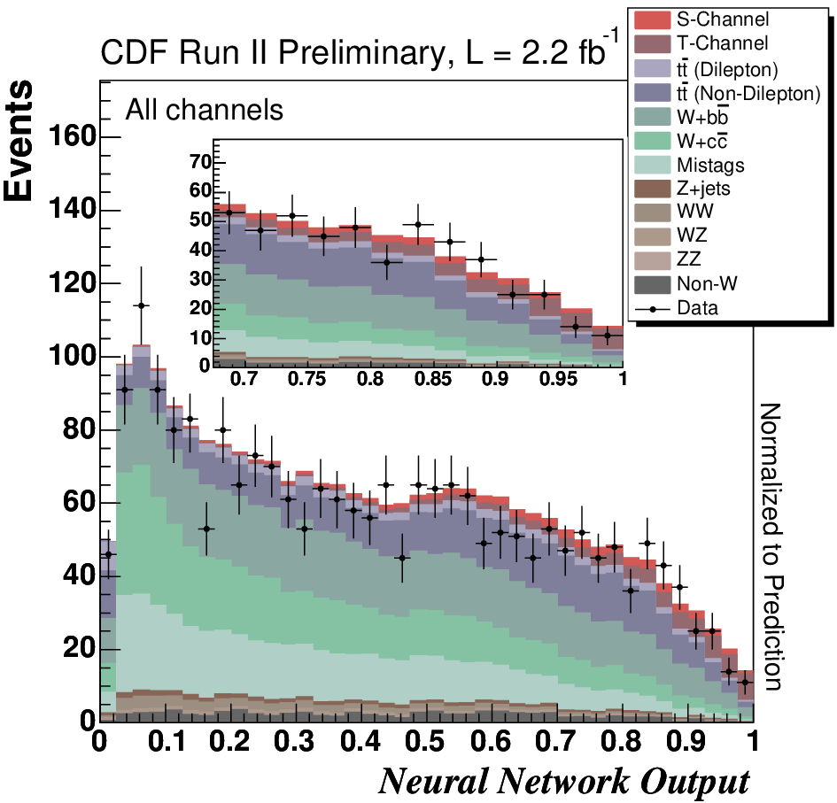
The NEAT combination method takes the discriminating variable from each analysis and combines them into one “super-analysis”. The new super-discriminant is a neural network in which the weights and topology are optimized for sensitivity by using a technique known as neuro-evolution of augmenting topologies (NEAT) [2]. A separate discriminant is optimized for events with two or three jets and events with one or two -tags. As in the individual analyses, templates based on the event-by-event output of NEAT are built for signal and background expectations and the data is fit to these to extract the most likely single top component. Figure 1 shows the expected composition of signal and background as well as the CDF data for all tag and jet channels combined.
III BLUE Combination
As a cross check to the NEAT combination, the method of forming a Best Linear Unbiased Estimate, BLUE, is used to make a weighted average of the three single top cross section measurements [3]. Recall a simple combination method:
| (1) |
where and are the measured value and error of the ith analysis, is the average of the measurements, is the column vector , and is the covariance matrix. In this case, is diagonal with . BLUE is based upon the formula above, but in order to combine measurements which each have different types of errors, is defined as
| (2) |
where is the th type of error on the th measurement and is the correlation of the th error between the th and th measurement.
The beauty of BLUE lies in the fact that a minimization routine on this need not be run to get the mean. After defining to be the inverse of the covariance matrix and as below, a weight for each measurement, , can then be calculated:
| (3) |
BLUE then predicts
| (4) |
where is the minimum of the and is the total error.
BLUE needs the measured values, uncertainties, and correlations between each analysis before the combined result can be calculated. Correlated pseudo-experiments are thrown from fully simulated events matched between each analysis and the correlations between analyses of the resulting cross sections measured in each pseudo-experiment are summarized in Table 1.
| LF | ME | NN | |
|---|---|---|---|
| LF (1.79 pb) | 1.0 | 0.599 | 0.741 |
| ME (2.17 pb) | — | 1.0 | 0.609 |
| NN (1.97 pb) | — | — | 1.0 |
In general, errors may have dependence on the value measured. Analyses which measure lower than expected could have a smaller error and this may bias the combination. In order to avoid this bias we run BLUE iteratively. Another complication is that errors need not be symmetric. Since BLUE is based on a Gaussian approximation it is not able to treat this directly. To handle this we use Asymmetric Iterative BLUE (AIB). AIB is a set of three BLUE combinations which uses average errors (for central value), upper errors, or lower errors as follows:
| (5) |
| (6) |
III.1 Results
The results of the the combination and each individual analysis are summarized in Figure 2. Fitting for the combined single-top cross section NEAT measures pb which corresponds to a measurement of . In addition the NEAT combination improves the expected sensitivity (-value [4])by about 9 %. The BLUE cross check measures a consistent cross section with NEAT and gains about 7 % in expected sensitivity. In addition, BLUE was used to study the consistency of the three analyses and finds that the combined measurement had a which was better than 87 % of pseudo-experiments. Also, about 15 % of pseudo-experiments thrown with the standard model expectation of single top events measured a cross section below 2.1 pb. So, BLUE confirms that the three CDF measurements are highly compatible with one another and that the combined result represents a deviation from the standard model expectation of about 1.
In summary, the three CDF analyses have been combined with two different techniques resulting in an improved sensitivity and measurement of the single top production cross section.

References
- [1] T. Aaltonen et al. [CDF Collaboration], arXiv:0809.2581 [hep-ex].
- [2] Kenneth O. Stanley and Risto Miikkulainen, Evolutionary Computation 10 (2) 99-127,2002.
- [3] L.Lyons, D. Gibaut, and P. Clifford, NIM A270, 110-117 (1988), L.Lyons, A. Martin, and D. Saxon, Phys. Rev. D 41, 3 (1990)
- [4] W.M. Yao et al. (Particle Data Group), J. Phys. G 33, 1 (2006).