Large-scale magnetic topologies of M dwarfs
Abstract
We present here the first results of a spectropolarimetric analysis of a small sample () of active stars ranging from spectral type M0 to M8, which are either fully-convective or possess a very small radiative core. This study aims at providing new constraints on dynamo processes in fully-convective stars.
Results for stars with spectral types M0-M4 – i.e. with masses above or just below the full convection threshold () – are presented. Tomographic imaging techniques allow us to reconstruct the surface magnetic topologies from the rotationally modulated time-series of circularly polarised profiles.
We find strong differences between partly and fully convective stars concerning magnetic field topology and characteristic scales, and differential rotation. Our results suggest that magnetic field generation in fully convective stars relies on different dynamo processes than those acting in the Sun and other partly convective stars, in agreement with theoretical expectations.
Keywords:
Stars: low-mass, brown dwarfs – Stars: magnetic fields – Stars: rotation – Stars: activity – Techniques: spectropolarimetricClassification:
97.20.Jg – 97.10.Ld – 97.10.Kc – 97.10.Jb1 Context
In partly convective stars such as the Sun, magnetic fields – the energy source of most activity phenomena – are induced by plasma motions: the combined action of differential rotation ( effect) and cyclonic convection ( effect) manages to generate a self-sustained magnetic field. The so-called dynamo [1] is believed to operate mostly through the tachocline, a thin zone of strong shear located at the interface between the radiative inner zone and the convective envelope [2].
Stars with masses lower than about are fully-convective [3] and thus do not possess a tachocline. However, they manage to trigger magnetic fields [4, 5, 6] and are very active [7, 8, 9]. Though significant progress was made since first non-solar dynamo mechanisms were proposed [10], theoretical and numerical modelling require observational constraints. It is now acknowledged, from observational [11, 12] and theoretical points of view [13, 14, 15], that fully convective stars (FCS) manage to yield large scale magnetic fields. But the properties of such magnetic fields, and their dependency on stellar parameters (in particular mass and rotation rate) are not yet clear.
We present here the first results of a spectropolarimetric analysis of a small sample of active M dwarfs with spectral types ranging from M0 to M8, which are either fully convective or possess a very small radiative core. We aim at exploring the properties of the large-scale magnetic topologies of FCS, and their evolution with main stellar parameters. The stars were selected from the rotation-activity study [7]. We chose only active stars so that the magnetic field is strong enough to produce detectable circularly polarised signatures, allowing us to apply tomographic imaging techniques. More details about the sample are available in Table 1.
| Name | ST | log | |||||||
|---|---|---|---|---|---|---|---|---|---|
| () | (km s-1) | (d) | (d) | () | () | (∘) | |||
| GJ 182 | M0.5 | 0.75 | 10 | 4.35 | 25 | 17 | 0.82 | 60 | |
| DT Vir | M0.5 | 0.59 | 11 | 2.85 | 31 | 9.2 | 0.53 | 60 | |
| DS Leo | M0 | 0.58 | 2 | 14.0 | 32 | 44 | 0.52 | 60 | |
| GJ 49 | M1.5 | 0.57 | 1 | 18.6 | 33 | 56 | 0.51 | 45 | |
| OT Ser | M1.5 | 0.55 | 6 | 3.40 | 35 | 9.7 | 0.49 | 45 | |
| CE Boo | M2.5 | 0.48 | 1 | 14.7 | 42 | 35 | 0.43 | 45 | |
| AD Leo | M3 | -3.18 | 48 | 4.7 | 0.38 | 20 | |||
| EQ Peg A | M3.5 | -3.02 | 54 | 2.0 | 0.35 | 60 | |||
| EV Lac | M3.5 | -3.33 | 64 | 6.8 | 0.30 | 60 | |||
| YZ CMi | M4.5 | -3.09 | 66 | 4.2 | 0.29 | 60 | |||
| V374 Peg | M4 | -3.20 | 72 | 0.62 | 0.28 | 70 | |||
| EQ Peg B | M4.5 | -3.25 | 76 | 0.53 | 0.25 | 60 |
For this study, we used the twin instruments ESPaDOnS on the 3.6-m Canada-France-Hawaii Telescope (CFHT) located in Hawaii and NARVAL on the 2-m Télescope Bernard Lyot (TBL) in southern France. These spectropolarimeters, built on the same design, can produce Stokes I,Q,U and V spectra spanning the entire optical domain (from 370 to 1000 nm) at a resolving power of [20].
We performed monitoring observations of the sample in circularly polarised light (Stokes ). Least-squares deconvolution (LSD) [21] was then applied, resulting, for each spectra, in a synthetic line profile gathering polarimetric information from most photospheric atomic lines.
2 Imaging procedure and Model description
For each star of the sample, our aim is to infer the topology of the surface magnetic field from the circularly polarised (Stokes ) LSD profiles we obtained. This can be achieved using a Zeeman-Doppler Imaging (ZDI) code [22]. The imaging process is based on the principles of maximum entropy image reconstruction. The magnetic field is decomposed into its poloidal and toroidal components, both expressed as spherical harmonics expansions. Starting from a null magnetic field, we iteratively improve our magnetic model by comparing the synthetic Stokes profiles with the observed LSD profiles, until we reach an optimal field topology that reproduces the data at a given level. The inversion problem being partly ill-posed, we use the entropy function to select the magnetic field with lowest information content among all those reproducing the data equally well [23].
To compute the synthetic Stokes profiles, the star is divided into a grid of cells on which the magnetic field components are computed directly from the coefficients of the spherical harmonics expansion. The contribution of each individual pixel is computed from a model based on Unno-Rachkovsky’s equations [18]. We then integrate all contributions from the visible hemisphere at each observed rotation phase.
While computing the Stokes profiles it is possible to account for differential rotation. For a given differential rotation law, each local line profile is Doppler-shifted as a function of the observation phase. It is then possible to investigate how the fit quality varies in a reasonable range of and values. We can thus derive the optimal , and corresponding error bars [24, 25, 12].
3 Reconstructed magnetic fields
For each star of our sample, we reconstruct with ZDI the large-scale surface magnetic field at least up to degree . We also measure differential rotation and assess time-variability of the magnetic topology whenever possible.
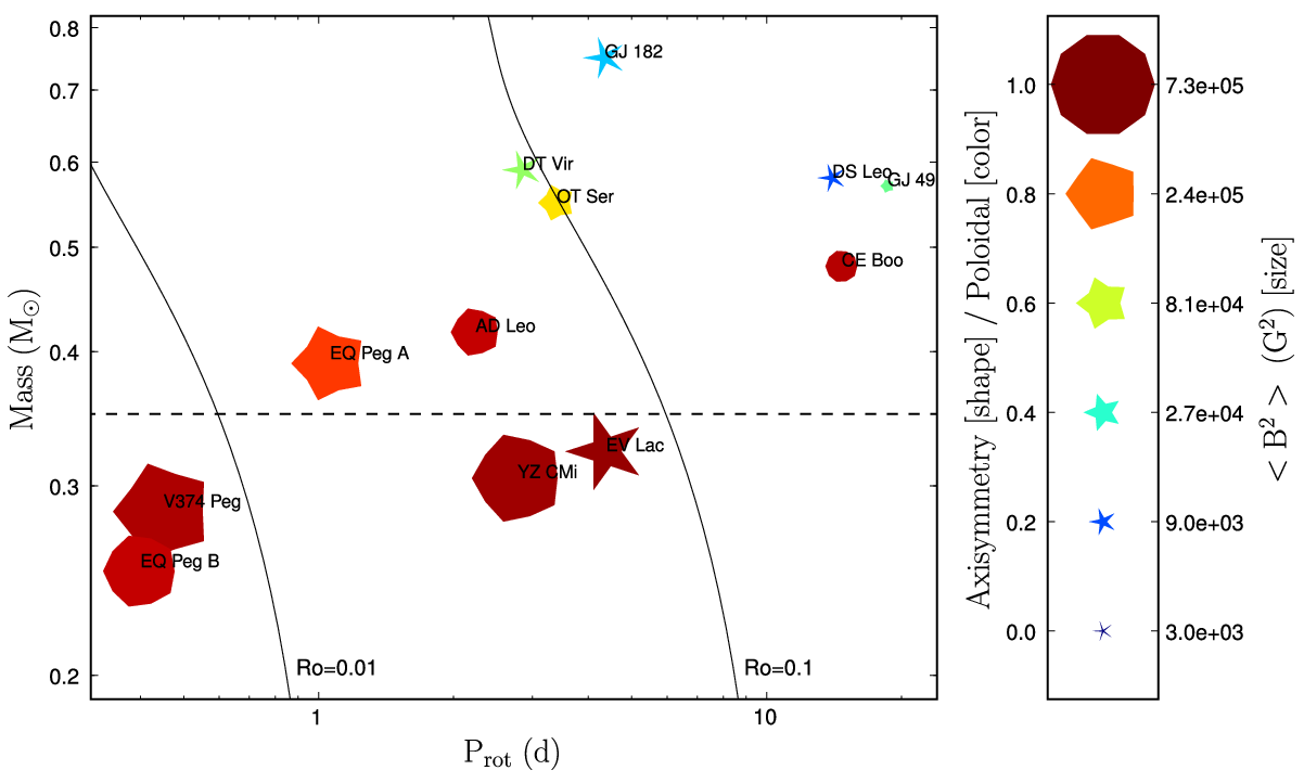
The field is characterised by three quantities: (a) the overall magnetic energy, (b) the ratio of magnetic energy reconstructed in the poloidal modes and (c) the ratio of poloidal magnetic energy reconstructed in the axisymmetric modes (defined by ). The results are described below and presented in a more visual way in Figure 1 as a function of and . See [Donati, these proceedings] for a version of this diagram including G and K dwarfs. To compare magnetic field generation in stars of different masses, it is convenient to introduce the effective Rossby number which rescales by a mass dependant coefficient. , where is an empirical convective turnover time inferred from X-ray luminosities [16]. On Fig. 1 we also plot contours of constant Rossby number and respectively corresponding approximately to the saturation and super-saturation thresholds (26, e.g.,).
The magnetic field topologies we reconstruct with ZDI and the differential rotation amplitudes are very different on each part of the boundary. This threshold is very sharp and well defined, with little apparent dependence with the rotation period. Typical examples of magnetic maps on each part of this limit are shown in Fig. 2.
 |
 |
For stars more massive than , we recover magnetic topologies including (i) a strong toroidal component and (ii) a high non-axisymmetric degree of the poloidal component. For 4 stars of this subsample we can derive differential rotation. We find , in agreement with the dispersion observed in previous photometric measurements of . As a consequence, surface magnetic features are short-lived, the topology completely changes on a timescale of a few months.
In the low mass subsample (¡), we reconstruct much stronger magnetic fluxes and very different large-scale magnetic topologies : (i) mostly poloidal ( of the reconstructed energy), (ii) strongly axisymmetric (except for EV Lac, more than half of the magnetic energy is reconstructed in modes) and (iii) close to a dipole with more 50% of the reconstructed magnetic energy lying in poloidal modes of degree . Very weak differential rotation is inferred from our data with 3 stars having of the order of a few mrad d-1. This very weak differential rotation is in agreement with the most recent numerical simulations [15]. These stars were observed at two different epochs separated by . Evolution of the magnetic topologies is small, in some cases, it is possible to fit observations separated by with a unique magnetic topology.
4 Conclusions and perspectives
Very different large-scale magnetic topologies are observed on each part of the limit. We also note that dynamo processes become suddenly much more efficient at triggering large-scale magnetic fields (see Fig. 1 and 3) at approximately the same mass (). This strong step is not visible in the log vs plot. This result suggests that (i) the X-ray emission is sensitive to overall magnetic energy whereas we are only sensitive to the largest scales. (ii) At a given stars with mass above or below generate comparable magnetic energy, but with very different spatial scales repartition (the less massive stars triggering more magnetic energy in the largest scales).
These strong changes in magnetic field generation occur at masses slightly larger than the theoretical limit to full convection (). This may be due to strong shrinking of the radiative inner zone predicted by theoretical models, from at to nothing at [17, 27].
We are currently completing this survey to extend it to fast rotators with , slow rotators with , two regimes not explored in the present sample. Present efforts are also directed to ultracool dwarfs (), to investigate how dynamo processes operate down to the brown dwarf limit, i.e. when stellar atmospheres start to become neutral.
 |
 |
References
- (1) E. N. Parker, ApJ 122, 293 (1955).
- (2) P. Charbonneau, Living Reviews in Solar Physics 2, 2 (2005).
- (3) G. Chabrier, and I. Baraffe, A&A 327, 1039–1053 (1997).
- (4) S. H. Saar, and J. L. Linsky, ApJ 299, L47–L50 (1985).
- (5) C. M. Johns-Krull, and J. A. Valenti, ApJL 459, L95 (1996).
- (6) A. Reiners, and G. Basri, ApJ 644, 497–509 (2006).
- (7) X. Delfosse, T. Forveille, C. Perrier, and M. Mayor, A&A 331, 581–595 (1998).
- (8) S. Mohanty, and G. Basri, ApJ 583, 451–472 (2003).
- (9) A. A. West, S. L. Hawley, L. M. Walkowicz, K. R. Covey, N. M. Silvestri, S. N. Raymond, H. C. Harris, J. A. Munn, P. M. McGehee, Ž. Ivezić, and J. Brinkmann, AJ 128, 426–436 (2004).
- (10) B. R. Durney, D. S. De Young, and I. W. Roxburgh, Solar Physics 145, 207–225 (1993).
- (11) J.-F. Donati, T. Forveille, A. C. Cameron, J. R. Barnes, X. Delfosse, M. M. Jardine, and J. A. Valenti, Science 311, 633–635 (2006).
- (12) J. Morin, J.-F. Donati, T. Forveille, X. Delfosse, W. Dobler, P. Petit, M. M. Jardine, A. C. Cameron, L. Albert, N. Manset, B. Dintrans, G. Chabrier, and J. A. Valenti, MNRAS 384, 77–86 (2008).
- (13) G. Chabrier, and M. Küker, A&A 446, 1027–1037 (2006).
- (14) W. Dobler, M. Stix, and A. Brandenburg, ApJ 638, 336–347 (2006).
- (15) M. K. Browning, ApJ 676, 1262–1280 (2008).
- (16) M. Kiraga, and K. Stepien, Acta Astronomica 57, 149–172 (2007).
- (17) I. Baraffe, G. Chabrier, F. Allard, and P. H. Hauschildt, A&A 337, 403–412 (1998).
- (18) J. Morin, J. . Donati, P. Petit, X. Delfosse, T. Forveille, L. Albert, M. Auriere, R. Cabanac, B. Dintrans, R. Fares, T. Gastine, M. M. Jardine, F. Lignieres, F. Paletou, J. C. Ramirez Velez, and S. Theado, ArXiv e-prints 808 (2008).
- (19) J. Donati, J. Morin, P. Petit, X. Delfosse, T. Forveille, M. Auriere, R. Cabanac, B. Dintrans, R. Fares, T. Gastine, M. Jardine, F. Lignieres, F. Paletou, J. Ramirez Velez, and S. Theado, ArXiv e-prints 809 (2008).
- (20) J.-F. Donati, “ESPaDOnS: An Echelle SpectroPolarimetric Device for the Observation of Stars at CFHT,” in Astronomical Society of the Pacific Conference Series, edited by J. Trujillo-Bueno, and J. Sanchez Almeida, 2003, vol. 307 of Astronomical Society of the Pacific Conference Series, p. 41.
- (21) J.-F. Donati, M. Semel, B. D. Carter, D. E. Rees, and A. C. Cameron, MNRAS 291, 658–682 (1997).
- (22) J.-F. Donati, and S. F. Brown, A&A 326, 1135–1142 (1997).
- (23) J. Skilling, and R. K. Bryan, MNRAS 211, 111 (1984).
- (24) P. Petit, J.-F. Donati, and A. Cameron, MNRAS 334, 374–382 (2002).
- (25) J.-F. Donati, A. Collier Cameron, and P. Petit, MNRAS 345, 1187–1199 (2003).
- (26) N. Pizzolato, A. Maggio, G. Micela, S. Sciortino, and P. Ventura, A&A 397, 147–157 (2003).
- (27) L. Siess, E. Dufour, and M. Forestini, A&A 358, 593–599 (2000).