Damping of the baryon acoustic oscillations in the matter power spectrum as a probe of the growth factor
Abstract
We investigate the damping of the baryon acoustic oscillations (BAO) signature in the matter power spectrum due to the quasi-nonlinear clustering of density perturbations. On the basis of the third order perturbation theory, we construct a fitting formula of the damping in an analytic way. This demonstrates that the damping is closely related with the growth factor and the amplitude of the matter power spectrum. Then, we investigate the feasibility of constraining the growth factor through a measurement of the damping of the BAO signature. An extension of our formula including higher order corrections of density perturbations is also discussed.
1 Introduction
The baryon acoustic oscillations (BAO) imprinted in the galaxy power spectrum have recently attracted remarkable attention, as a useful probe for exploring the origin of dark energy [1, 2]. The BAO signature has been clearly detected in the 2dFGRS and the SDSS galaxy samples [3, 4, 5, 6, 7]. The feasibility of constraining the equation of state parameter of dark energy is demonstrated [8, 9, 10], where is defined by , where and are the pressure and the energy density of the dark energy component, respectively. Furthermore, a lot of BAO survey projects are under progress, or planned [11, 12, 13, 14, 15, 16].
Though these BAO surveys will precisely measure the galaxy power spectra, but we also need precise theoretical templates, in order to obtain a useful cosmological constraint from observational data. In practice, we need to solve uncertainties about the gravitational nonlinear clustering of the density perturbations, the redshift-space distortions, and the galaxy clustering bias, because these uncertainties might yield some systematic effects in the BAO signature. Then, a lot of works related to these topics have been done recently, which are very important and challenging for future research of dark energy [17, 18, 19, 20, 21, 22, 23, 24, 25, 26, 27].
In the present paper, we focus on the damping of the BAO signature in the matter power spectrum due to the nonlinear gravitational clustering. We investigate this damping in a semi-analytic way on the basis of the third order perturbation theory of density fluctuations. The nonlinear clustering is a consequence of mode-couplings of the density fluctuations and the peculiar velocity divergence in Fourier space. Especially, we demonstrate how the damping of the BAO signature can be expressed with/without and , which describe the mode-coupling (see sections 2 and 3). Then, we develop a simple fitting formula relevant to the damping, which demonstrates the fact that the damping of the BAO signature is closely related with the growth factor and the amplitude of the matter power spectrum. This suggests that a measurement of the damping of the BAO signature might be a probe of the growth factor of the density fluctuations, though we need to further investigate if the effects of the redshift-space distortion or the galaxy clustering bias are influential to the damping.
This paper is organized as follows; In section 2, we briefly review the third order perturbation theory, and derive the second order power spectrum. In this formalism, the nonlinear gravitational clustering is described by the coupling of the Fourier modes of the density fluctuations and the peculiar velocity divergences. In section 3, we investigate the damping of the BAO signature due to the coupling of the Fourier modes in an analytic way. And a fitting formula of the damping, applicable in weakly nonlinear regime, is developed. The formula is compared with a result of -body simulation. Extensions of the formula are also discussed. In section 4, with the use of the fitting formula, we demonstrate a future feasibility of constraining the growth factor through a measurement of the damping of the BAO signature. The last section is devoted to a summary and conclusions. Throughout this paper, we use the unit in which the velocity of light equals 1, and adopt the Hubble parameter with , unless explicitly stated.
2 Quasi-nonlinear evolution of the matter power spectrum
To investigate the effect of the nonlinear gravitational clustering in the present work, we employ the standard perturbation theory (SPT) of the density fluctuations and the peculiar velocity divergences [28, 29, 30, 31, 32, 33, 34, 35, 36]. Numerical simulation is a rigorous approach to the gravitational clustering, but the perturbative approach has an advantage to understand which factors are relevant to the damping of the BAO signature in an analytic way. Recently, several authors have developed new formalism beyond the SPT [37, 38, 39, 40, 41, 42, 43, 44, 45, 46]. In the later subsection 3.3, we discuss a possible extension of our main result to include these formalism. However, let us start with briefly reviewing the derivation of the second order power spectrum on the basis of the SPT up to the third order of perturbations.
We consider the matter fluctuations after the recombination whose wavelength of interest is smaller than the horizon size, then the evolution of the matter fluctuations can be analyzed by the pressure-less nonrelativistic fluid with the Newtonian gravity. Denoting the comoving coordinates by , and the conformal time by , the evolution equations are
| (1) | |||
| (2) | |||
| (3) |
where is the density contrast, is the peculiar velocity, is the gravitational potential, is the scale factor, a dot denotes the derivative with respect to the conformal time, and . Here, the Einstein-de Sitter universe is assumed.
We ignore the rotational mode of the velocity, since our interest is only the growing solution, and the rotational mode is the decaying solution in the expanding universe. Then, we introduce the velocity divergence,
| (4) |
It is convenient to analyze the perturbations in the Fourier space, and we define the Fourier coefficients as
| (5) | |||
| (6) |
Then, equations (1) - (3) yield
| (7) | |||
| (8) |
where denotes the Dirac’s delta function. The right hand side of these equations describes the mode-couplings which govern the nonlinear evolution of the matter fluctuations.
To solve these coupled equations, we adopt the perturbative expansion as
| (9) |
In general, the -th order solution can be written as
| (10) | |||
| (11) |
where and are defined as
| (12) | |||
Assuming that the first order density perturbations described by is a Gaussian random field, we obtain the second order matter power spectrum
| (14) |
where is the linear power spectrum given by
| (15) |
is the linear growth factor, and is the second order contribution to the power spectrum, which is conventionally expressed as follows;
| (16) |
Taking the 4-point correlations of into consideration, we obtain the explicit form of expressed as the integral of the square of the linear power spectrum,
| (17) |
where is symmetrized over its arguments. On the other hand, has the form slightly different with ,
| (18) |
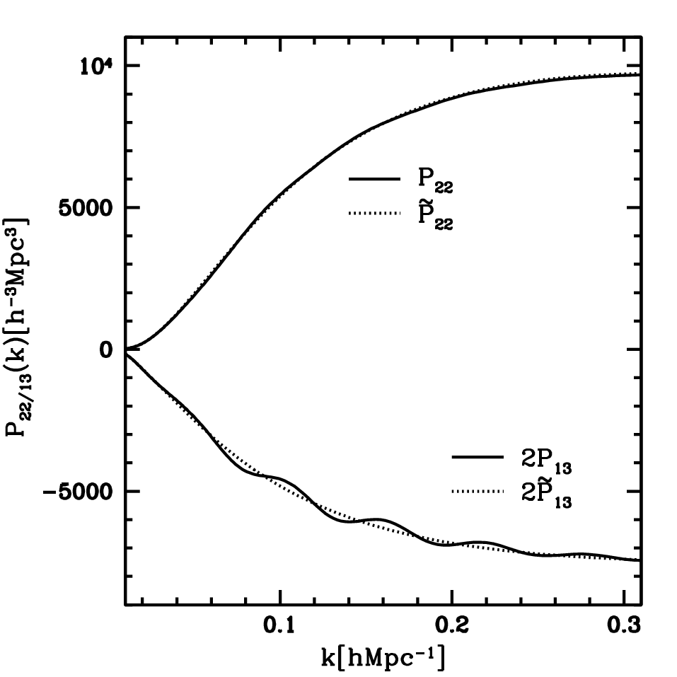
The solid curve in figure 1 shows typical behaviour of and , where the cosmological parameters are , , , and . We discuss further details of the typical behaviour of and in the next section.
Originally, this perturbation expansion is consistently formulated in the Einstein de-Sitter universe. The result is extensively used for the other general cosmological model, with the corresponding growth factor normalized as at . We follow this prescription because the validity of the extensive use of the result is known, for example, in the literature [36, 47].
3 Damping of the BAO signature
In this section, we will examine the damping of the BAO signature due to the nonlinear gravitational clustering with employing the third order perturbation theory. The BAO signature in the matter power spectrum can be extracted as follows:
| (19) |
where is the matter power spectrum including the BAO signature, but is the matter power spectrum without the BAO, which is calculated using the no-wiggle transfer function in [48]. Hereafter, the quantity with the ’tilde’ implies the quantity computed using the no-wiggle transfer function. Within the third order perturbation theory, we may write
| (20) |
where is
| (21) |
and and are, respectively, defined by (17) and (18), but with the no-wiggle transfer function.
Figure 2 shows as a function of the wavenumber for several redshifts, which is obtained using the third order perturbation theory (see also below). Here, the spatially flat universe with the cold dark matter (CDM) and the cosmological constant is assumed, where the cosmological parameters are the same as those of Figure 1. The oscillating behaviour of the curves is the BAO signature. As the redshift becomes small, one can see that the amplitude of the oscillations decreases. This damping of the oscillations is more significant as is larger.
3.1 Analytic approach
The aim of this paper is to understand the nature of the damping of the BAO signature in detail. To this end, the analytic approach based on the third order perturbation theory is useful. With the use of the formula of the second order power spectra, (14) and (20), we have
| (22) |
First, we adopt an approximation,
| (23) |
In brief, in (16) is replaced with . The validity of this approximation is demonstrated in figure 1, where the upper solid curve is , and the upper dotted curve is . The validity of this approximation comes from the fact that the mode-coupling of different Fourier modes decrease the coherent BAO signature. As shown in this figure, the tiny oscillatory feature remains. This may induce somewhat the small shift of the peaks(troughs) of the BAO, as mentioned in the reference [41]. However, this shift of peak location would not be problematic, as long as we are interested in the damping of the BAO signature.
On the other hand, can not be simply replaced with . However, careful consideration leads to an expression for in terms of the linear power spectrum multiplied by a monotonically decreasing function, as follows. First, we define
| (24) |
which corresponds to (22), within the linear theory of density fluctuations. Note that is not time-dependent. With this definition, we obtain
| (25) |
Here, we apply the following approximation to the linear power spectrum of the integrand,
| (26) | |||||
Substituting (26) into (23), is written as
| (27) |
Then, from (22), we obtain
| (28) |
This formula indicates how the BAO signature is modified as the gravitational clustering evolves, which is expressed by the BAO signature in the linear theory multiplied by the correction determined by the no-wiggle quantities and the growth factor. The second term of the denominator in (28) is small within the perturbation scheme, we may expand it as
| (29) |
though the higher order terms make no sense because we are working in the second order theory of the power spectrum. The expression (29) indicates that the leading effect of the nonlinear mode-coupling on the damping is described by the factor , and that the sign of the term clearly shows that this effect is a damping.
3.2 Fitting formula
As we are working within the third order perturbation theory, its prediction does not perfectly coincide with the result of full order computation, which can be obtained by -body simulations. However, we believe that the prediction of the third order perturbation theory is useful in constructing a semi-analytic formula which reproduces the result of -body simulations. Then, we here find a simple fitting formula which reproduces the prediction of the third order perturbation theory. We discuss the validity of the formula in comparison with a -body simulation in the below.
Up to the second order of , (29) yields
| (30) |
From a detailed analysis of as a function of , we find that the following fitting formula works well,
| (31) |
where is the rms matter density fluctuations averaged over the sphere with the radius of , and are the constant parameters which depend on , and . Figures 3 and 4 show the best-fit value of and as a function of and , where we fixed . This shows that these two parameters depend on and linearly. We can show a similar dependence on . Then, we found the following fitting formula:
| (32) | |||
| (33) |
Though these dependence on the cosmological parameter might have to be investigated more carefully, but the validity is guaranteed in the following narrow range
| (34) | |||
| (35) | |||
| (36) |
In the present paper, we simply assume that the dependence on the other cosmological parameters except for , and can be ignored.
Finally, we obtain the heuristic expression of the leading correction for the BAO signature,
| (37) |
with
| (38) |
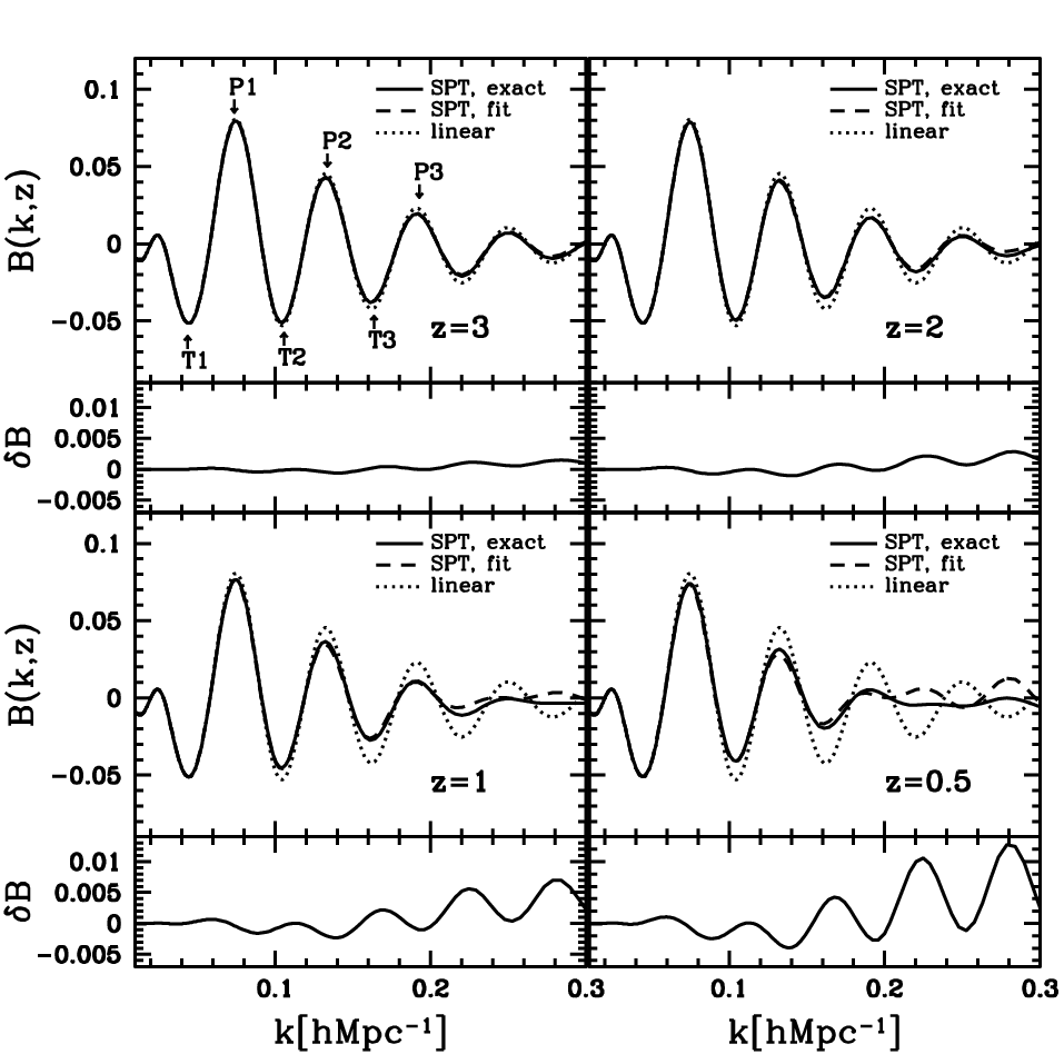
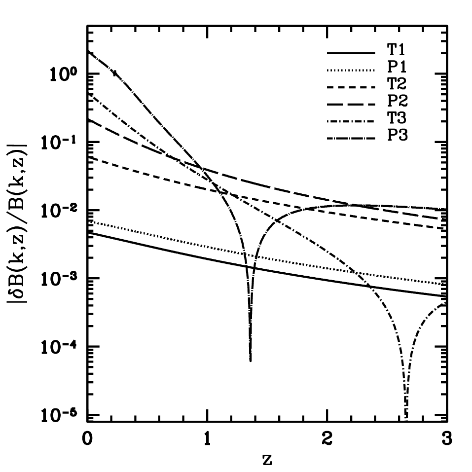
Figure 5 demonstrates the agreement between this fitting formula, , and the prediction of the third order perturbation theory, , (22). As one can see from this figure, the agreement becomes worse as the redshift is lower and the wavenumber is larger. Figure 6 shows the relative error of the fitting formula, , as a function of the redshift at the wavenumbers of P1, P2, P3, T1, T2 and T3, which are defined in Figure 5. The relative error is about less than at worst in the range of the wavenumber until . The sign of of the third peak (trough) changes around the redshift 2.7 (1.4), where the relative error becomes zero. For the redshift less than , the agreement becomes worse especially at the large wavenumber . However, we should also note that the third order perturbation theory becomes worse to reproduce -body simulations for lower redshift and for larger wavenumbers.
Figure 7 shows a comparison of our fitting formula (, solid curve) and a result of -body simulation (squares with error bar) [49]. This demonstrates that our fitting formula reproduces the result of -body simulation for until within error bars, roughly. In this conclusion, note that we focus on the damping of the BAO signature, not on the amplitude of the power spectrum itself.
In the -body simulation, we adopt a CDM cosmology (, , , , , ; WMAP5 best fit value, [50]), and calculate the linear matter power spectrum using CAMB [51]. We adopt particles in periodic cubes with each side , and displace -body particles using the second-order Lagrangian perturbation theory (e.g., [52]) from uniform grid positions at . The simulations are carried out using the Gadget2 code [53] to output data of redshifts (, , , and ). Our total simulation volume is Gpc3, which might be small to investigate our scales of interest (first a few BAO peaks). Then we correct the deviations from the ideal case of infinite volume, as follows.
In addition to the time integration using Gadget2, we also calculate the time evolution of the density contrast using the second-order perturbation theory starting from the identical initial condition with that used for the -body simulation. We then calculate the power spectrum from the result of the perturbation theory, and measure the deviation from the the linear power spectrum at each output time. The deviation of our finite volume simulation is well explained by the mode-couplings predicted by the second-order perturbation theory. Then, we can obtain a corrected power spectrum by multiplying the measured power spectrum from -body simulations by the ratio of the linear power spectrum to the power spectrum predicted by the perturbation theory. Thus the error bars in the figure stand for the remaining standard errors after this correction, which are very small compared with the usual cases in the region of the small wavenumbers. This is because the perturbation theory used for the correction is more accurate at the small wavenumbers, which can remove the deviations from the linear power spectrum better. This correction does not improve the errors at large wavenumbers (see [24], [49] for more details). Moreover, in order to construct the no-wiggle spectrum required for computing the ratio , we use a cubic basis-spline fitting with the same break points as in [27] (see also [8]).
3.3 Possible extension and discussion
There are other possible effects which may affect the damping of the BAO signature: the higher order nonlinear effect, the redshift-space distortions and the clustering bias. These effects may be influential to the damping of the BAO signature, however, there remains a lot of uncertainties about these effects, at present. Here, let us consider a possible extension of our work to include the higher order nonlinear corrections in real space.
The standard perturbation theory is useful to analyse the damping of the BAO signature in an analytic way, however, it is not enough for precise predictions that match with result of -body simulations in the regime where the nonlinear effect becomes significant. Recently, several authors have developed non-perturbative approach to the nonlinear density clustering, as mentioned above [37, 38, 39, 40, 41, 42, 43, 44, 45, 46].
As an alternative to the SPT, we here consider the work proposed by [46], which uses the technique of resumming infinite series of higher order perturbations on the basis of the Lagrangian perturbation theory (LPT). One of the advantage of this approach is the simplicity of the resulting expression of the nonlinear power spectrum, which enable us to incorporate the result into our formula. In the framework of the LPT[46], the matter power spectrum can be given by
| (39) |
where
| (40) |
Corresponding to (22), we define the BAO signature of the matter power spectrum based on the LPT,
| (41) |
where is defined by (39) but with the no-wiggle transfer function. Adopting an approximation, , we can obtain the following expression
| (42) |
Repeating the same procedure from (28) to (30), one can obtain the leading correction to the BAO
| (43) |
then we obtain
| (44) |
as an extended fitting formula. Note that this reduces to the expression (30) in the limit of . Comparing (44) and (37), the difference is the contribution from in the denominator in front of . Since is positive, this correction make the damping of the BAO signature weaker compared with (37). In figure 7, the dashed curve plots , (44).
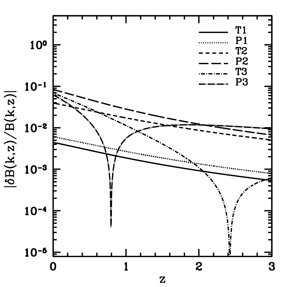
In order to show the validity of the fitting formula, figure 8 plots the relative error s at the wavenumber of the peaks and troughs as a function of the redshift, which is the same as Figure 6 but with the LPT instead of the SPT. As one can see from this figure, the fitting function better reproduces the damping of the BAO signature , compared with the case of the SPT, especially for larger wavenumber even at lower redshift. The relative error is less than in the range of the wavenumber (near the third peak) until the present epoch, . In the below, we investigate other possible ways in describing the damping of the BAO signature due to the nonlinear effect.
One of the other possible formulas for the fitting function is the exponential function, as has been discussed in references (e.g., [7, 20, 22, 54]). Angulo et al [22] discussed the following fitting formula with the Gaussian damping function,
| (45) |
where is a time-dependent free parameter, which should be calibrated by measurements from -body simulations. This free parameter describes the time-dependence of the BAO damping, and Sanchez et al [54] obtained the best fit value, at , from their result of -body simulations in [21]. Their model includes another parameter, , which describes the shift of the BAO scale in the wavenumber. However, in the present paper, we adopt the case of no shift of the BAO scale () because our interest is focused on the damping of the BAO signature not on the shift of the BAO scale. It is also shown that almost equals 1 [21].
Figure 9 compares our fitting functions and the Gaussian damping function. The vertical axis stands for divided by , which means the damping function. The dotted curve and the solid curve are and , respectively. The dashed curve is the Gaussian damping function, (45), with . becomes negative as the wavenumber becomes larger, . This is because the phase inversion of the BAO signature appears in the SPT, as shown in the panel of in Figure 5, where of the SPT breaks down in this regime as mentioned in Section 3.2. On the other hand, the damping function based on the LPT, , shows the similar behavior as the Gaussian damping function, which approaches zero in the limit of . This is due to the modification by the factor, , in (44). becomes negative for because of the same reason as that for .
In figure 9, we also plot the following damping function (dot-dashed curve),
| (46) |
The leading term of the expansion of this damping function with respect to leads to , (37). As one can see, this damping function agrees with the Gaussian damping function, (45). This means that the higher order perturbations is important in describing the BAO signature for the regime of the wavenumber, at redshift .
The result of this section gives us a clue to find how to describe the BAO damping due to the nonlinear gravitational clustering. The BAO damping is determined by the normalization and the growth factor . This suggests that a measurement of the BAO damping might be useful to estimate the growth factor of the amplitude of the density perturbations, . In section 4, we demonstrate a feasibility of constraining by measuring the damping of the BAO signature.
4 Feasibility of Constraining
As shown in the previous section, the damping of the BAO signature is closely related with the amplitude of the power spectrum, which is determined by , while the BAO signature within the linear theory is determined by the density parameters and . In this section, we discuss the feasibility of constraining by measuring the damping of the BAO in the power spectrum in quasi-nonlinear regime. To this end, the formula developed in the previous section is useful.
As mentioned in section 1 and subsection 3.3, the redshift-space distortions and the clustering bias might be additionally influential to the damping of the BAO signature. However, we here assume an optimistic case that the damping is determined by the quasi-nonlinear clustering effect and neglect the effects on the damping of the BAO signature from the redshift-space distortions and the clustering bias. Then, we study how a measurement of the damping is useful to determine . Very recently, it is recognized that a measurement of the growth factor of the density perturbations is a key to distinguish between the dark energy model and modified gravity model for the cosmic accelerated expansion (e.g., [55, 56], and references therein). Our investigation is the first step to investigate if a measurement of the BAO damping is useful to measure the growth factor.
In our investigation, we adopt a simple Monte Carlo simulation of the galaxy power spectrum assuming the CDM model. The error of the galaxy power spectrum depends on its amplitude. For definiteness, we assume the galaxy power spectrum is modeled with the no-wiggle linear power spectrum in real space, , as
| (47) |
with
| (48) |
where we use (44) as , is a constant bias factor, and , and are the parameters, which describe the correction of the nonlinear clustering, the redshift-space distortions and the scale-dependent bias to the no-wiggle power spectrum. This model is based on the -model of Cole et al [57], and is elaborated by Sanchez et al [54] by adding the new parameter which better reproduces the nonlinear power spectrum at large wavenumber. Cole et al [57] showed that, from numerical study, the value of is adequate to reconstruct the galaxy power spectrum in redshift-space, though strongly depends on the galaxy type [57, 58, 59]. Then, for simplicity, we here adopt and consider the cases , to estimate the error for the galaxy power spectrum. We assume the bias parameter , for simplicity.
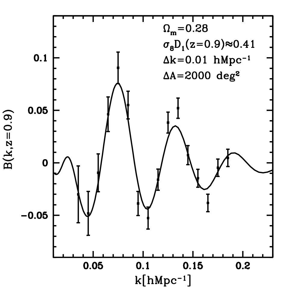
To estimate the constraint on the growth factor, we perform a simple Monte-Carlo simulation. We assume that the BAO signature, , can be extracted from a galaxy power spectrum by the method like in the reference [5]. The variance of the error in measuring the BAO signature can be estimated by
| (49) |
with
| (50) |
where is the volume of the shell in the Fourier space, and is defined as
| (51) |
where is the comoving mean number density, is the comoving distance-redshift relation, and is the survey area.
With the use of the above formulas, we assess defined by
| (52) |
where is the theoretical one of a fiducial target model at the wavenumber , while is the corresponding observational one. The fiducial target model is and , , , and , which are the same as those adopted in figure 1. is obtained through a Monte Carlo simulation, following the steps in the below,
- 1.
Based on the fiducial model, compute and the variance at , for . Here we specify a bin of the Fourier space, , and consider the range of , where the validity of our formula in the previous section is guaranteed. We assume two galaxy redshift samples as typical future survey. One is the WFMOS-like sample, in the range of redshift , and , which contains galaxies. The other sample assumes the same number density and the range of the redshift, but the larger survey area steradian.
- 2.
Each is obtained through a random process assuming the Gaussian distribution function with the variance . The data points in figure 10 show an example of a set of generated through the random process.
- 3.
We assess the values of with this sample obtained by the step (i) and (ii).
We iterate these steps and compute 1000 sets of , then obtain the average of . For the theoretical model, , we fixed , , and as those of the fiducial model, but took and as the variable parameters. Solid curves in figure 11 show the contour of (inner curve) and (outer curve), which corresponds to the and the statistical confidence level, respectively, in the and plane, for the WFMOS-like galaxy sample of . The dotted curves show the same but with the sample of the survey area steradian.
From figure 11, one can read that the 1 error of is about for the sample of , and is about for the sample of steradian. Thus, the constraint on of the WFMOS-like sample () is not very stringent. We already have the small uncertainty of at the level of a few [36], from the result by the WMAP observations, which is obtained on the basis of the flat CDM cosmological model with the cosmological constant. However, we note that the BAO damping is unique and independent to obtain a constraint on around the redshift .
It would be useful to discuss the origin of the error. To this end, we adopt the Fisher matrix approach. As we are considering the constraint from the damping of the BAO signature, we may work with the formula for the Fisher matrix
| (53) |
where denotes cosmological parameters, for which we focus on and , is defined by (48), is defined by (51), we adopt (44) as , and and . The minimum error attainable on is expressed by the diagonal part of the inverse Fisher-matrix, , if the other parameters are known. Figure 12 plots the errors and , obtained from the Fisher-matrix, as a function of the mean number density .11 1 Note that the Fisher-matrix depends on the parameter . The thick (thin) solid curve is of the sample with ( radian). The dotted curve is . Here we adopted , but the result is not sensitive to this choice. One can read that the value of the error at the point is consistent with the result of figure 11.
Figure 12 demonstrates that the constraint can be improved by increasing the number density of the galaxy sample, but can not be improved for . The reason can be explained using figure 13, which plots as a function of the wavenumber, where we fixed . In the region , we have , which means that the shotnoise is not the dominant component of the error. However, the constraint on the parameter is slightly improved by increasing the number density , depending on the bias .
Finally in this section, we mention the effect of the redshift-space distortions and the clustering bias on the BAO damping, which might be influential in measuring . It would be true that there still remains room to investigate how the redshift-space distortions and the clustering bias affect the BAO damping. If the effect of the redshift-space distortions and the clustering bias on the BAO damping could not be clarified, it would make it difficult to conclude that the BAO damping is useful. However, very recently, several authors have discussed the issue [54, 60, 61]. If the effect on the BAO damping are well understood, it can be a signal, and would be useful in measuring the growth factor.
5 Summary and Conclusions
In the present paper, we examined the effect of the nonlinear gravitational clustering on the BAO signature in the matter power spectrum. In particular, we focused on the damping of the BAO signature in the quasi-nonlinear regime. Our approach is based on the third order perturbation theory of the matter fluctuations, which enables us to investigate the damping in an analytic way. We found a simple analytic expression that describes the damping of the BAO signature, which clarifies what the important factor is for the damping. We showed that the leading correction for the damping is in proportion to the combination of . On the basis of the result, we constructed a fitting formula for the correction of the damping of the BAO signature in the weakly nonlinear regime, which is expressed as a function of , , and . This fitting formula reproduces the damping of the BAO signature of the second order power spectrum within the standard perturbation theory at level for until , though the formula is only guaranteed in a narrow range of the parameters , and .
We also discussed a possible extension of our formula to elaborate higher order nonlinear corrections using a technique of resumming infinite series of higher order perturbations on the basis of the Lagrangian perturbation theory. This extended formula reproduces the damping of the BAO signature of the second order power spectrum based on the Lagrangian perturbation theory at level for until . This formula was compared with a result of -body simulation, which showed the validity of the extended formula.
A measurement of the damping of the BAO signature might be useful as a probe of the growth factor of the density fluctuations. As a first step to investigate such the possibility, we assessed the feasibility of constraining by measuring the damping of the BAO in the power spectrum. For a useful constraint, we need a very wide survey area of the sky. For a definite conclusion, however, we must include the effect of the redshift-space distortions and the galaxy clustering bias on the damping of the BAO signature. Thus, more sophisticated formula including the effect of the redshift-space distortions and the galaxy clustering bias at the same time is required. If this effect on the BAO damping was well understood, it can be useful in measuring the growth factor. We plan to revisit this issue in future work.
References
References
- [1] Albrecht A et al, 2006 arXiv:astro-ph/0609591
- [2] Peacock J A et al, 2006 arXiv:astro-ph/0610906
- [3] Eisenstein D J et al, 2005 Astrophys. J. 633 560
- [4] Hetsi G, 2006 Astron. Astrophys. 449 891
- [5] Percival W J et al, 2007 Astrophys. J. 657 645
- [6] Percival W J et al, 2007 Astrophys. J. 657 51
- [7] Tegmark M et al, 2006 Phys. Rev. D 74 123507
- [8] Percival W J et al, 2007 Mon. Not. R. Astron. Soc. 381 1053
- [9] Okumura T et al, 2008 Astrophys. J. 677 889
- [10] Hetsi G, 2006 Astron. Astrophys. 459 375
- [11] http://www.sdss3.org/
- [12] Totani T, 2006 private communication
- [13] Bassett B A, Nichol R C and Eisenstein D J (the WFMOS Feasibility Study Dark Energy Team), 2005 arXiv:astro-ph/0510272
- [14] http://www.lsst.org/
- [15] http://www.skatelescope.org/
- [16] Robberto M et al, 2007 arXiv:0710.3970
- [17] Seo H-J and Eisenstein D J, 2003 Astrophys. J. 598 720
- [18] Seo H-J and Eisenstein D J, 2005 Astrophys. J. 633 575
- [19] Seo H-J and Eisenstein D J, 2007 astro-ph/0701079
- [20] Seo H-J et al, 2008 arXiv:0805.0117
- [21] Angulo R et al, 2005 Mon. Not. R. Astron. Soc. Lett. 362 L25
- [22] Angulo R et al, 2008 Mon. Not. R. Astron. Soc. 383 755
- [23] Shoji M et al, 2008 arXiv:0805.4238
- [24] Takahashi R et al, 2008 arXiv:0802.1808
- [25] Wang Y, 2006 Astrophys. J. 647 1
- [26] McDonald P and Eisenstein D, 2007 Phys. Rev. D76 063009
- [27] Nishimichi T et al, 2007 Publ. Astron. Soc. Japan 59 1049
- [28] Juszkiewicz R, 1981 Mon. Not. R. Astron. Soc. 197 931
- [29] Vishniac E T, 1983 Mon. Not. R. Astron. Soc. 203 345
- [30] Fry J N, 1984 Astrophys. J. 279 499
- [31] Goroff M H et al, 1986 Astrophys. J. 311 6
- [32] Makino N, Sasaki M and Suto Y, 1992 Phys. Rev. D 46 585
- [33] Jain B and Bertschinger E, 1994 Astrophys. J. 431 495
- [34] Bernardeau F, Colombi S, Gaztanaga E and Scoccimarro R, 2002 Phys. Rep. 367 1
- [35] Saito S, Takada M and Taruya A, 2008 Phys. Rev. Lett. 100 191301
- [36] Jeong D and Komatsu E, 2006 Astrophys. J. 651 619
- [37] Valageas P, 2004 Astron. Astrophys. 421 23
- [38] Valageas P, 2007 Astron. Astrophys. 465 725
- [39] Crocce M and Scoccimarro R, 2006 Phys. Rev. D 73 063519
- [40] Crocce M and Scoccimarro R, 2006 Phys. Rev. D 73 063520
- [41] Crocce M and Scoccimarro R, 2008 Phys. Rev. D 77 023533
- [42] McDonald P, 2007 Phys. Rev. D 75 043514
- [43] Matarrese S and Pietroni M, 2007 J. Cosmol. Astropart. Phys. JCAP06(2007)026
- [44] Izumi K and Soda J, 2007 Phys. Rev. D 76 083517
- [45] Taruya A and Hiramatsu T, 2007 arXiv:0708.1367
- [46] Matsubara T, 2008 Phys. Rev. D 77 063530
- [47] Bernardeau F, 1994 Astrophys. J. 433 1
- [48] Eisenstein D J and Hu W, 1998 Astrophys. J. 496 605
- [49] Nishimichi T et al, 2008 arXiv:0810.0813
- [50] Komatsu E et al, 2008 arXiv:0803.0547
- [51] Lewis A et al, 2000 Astrophys. J. 538 473
- [52] Crocce M et al, 2006 Mon. Not. R. Astron. Soc. 373 369
- [53] Springel V, 2005 Mon. Not. R. Astron. Soc. 364 1105
- [54] Sanchez A G et al, 2008 arXiv:0804.0233
- [55] Yamamoto K et al, 2007 Phys. Rev. D 76 023504
- [56] Yamamoto K, Sato T and Hütsi G, 2008 Prog. Theor. Phys. 120 609
- [57] Cole S et al, 2005 Mon. Not. R. Astron. Soc. 362 505
- [58] Sanchez A G and Cole S, 2008 Mon. Not. R. Astron. Soc. 385 830
- [59] Hamann J et al, 2008 J. Cosmol. Astropart. Phys. JCAP07(2008)017
- [60] Matsubara T, 2008 arXiv:0807.1733
- [61] Jeong D and Komatsu E, 2008 arXiv:0805.2632