Effective Theory of Braid Excitations of Quantum Geometry in terms of Feynman Diagrams
Abstract
We study interactions amongst topologically conserved excitations of quantum theories of gravity, in particular the braid excitations of four valent spin networks. These have been shown previously to propagate and interact under evolution rules of spin foam models. We show that the dynamics of these braid excitations can be described by an effective theory based on Feynman diagrams. In this language, braids which are actively interacting are analogous to bosons, in that the topological conservation laws permit them to be singly created and destroyed. Exchanges of these excitations give rise to interactions between braids which are charged under the topological conservation rules.
1 Introduction
A substantial amount of work[1, 2, 3, 4, 5, 6, 7, 8, 9] has been done recently towards emergent matter as topological invariants of framed spin networks, embedded in a topological three-manifold[1, 2, 3, 4, 5, 6, 7, 8] and unembedded[9], as fundamental states of quantum gravity and quantum geometry. Some papers study the case of framed three-valent spin networks[1, 2, 3, 9], which were motivated by the pioneer work of Bilson-Thompson [10]. Others investigate the three-strand braids of four-valent spin networks embedded in a topological three manifold[5, 6, 7, 8].
The aim of this paper is to present an effective description of these emergent local excitations[11, 1, 5] in the language of Feynman diagrams. As an analogy effective emergent degrees of freedom have been realized in condensed matter physics. For example, there are emergent quasiparticles as collective modes in some condensed matter systems, such as phonons and rotons in superfluid He4. Another example is the string-net condensation which gives rise to low energy effective gauge theories[14].
The three-valent case considered in [1, 2, 3] is limited by lack of creation and annihilation of the topological invariants[2] which are considered corresponding to Standard Model particles[3]. This partly motivates our work in the four-valent case[4, 5, 6, 7, 8] in which the topological excitations can propagate and interact under the dual Pachner moves[5]. The four-valent spin networks here can be understood as those naturally occur in spin foam models[12], or in a more generic sense as the original proposal of spin networks put forward by Penrose[13]. Another motivation of working with four-valent spin networks is that the vertices correspond to three-dimensional space11 1 Note that this correspondence is only between a 4-valent vertex and a 3d simplicial complex. The precise correspondence with a (continuum) physical 3d space remains a big open question..
The dynamical entities being studied in the four-valent case are three-strand braids, each of which is formed by the three common edges of two adjacent nodes of a spin network. With the graphic notation and the classification of these three-strand braids obtained in [4], [5] discovers that stable three-strand braids, which are thought to be local excitations[5] exist under certain stability condition. Among the stable braids, there is a small class of braids, called propagating braids, which can propagate on the spin network. The braid propagation is chiral, in the sense that some braids can only propagate to their left in their ambient local graphs, whereas some only propagate to their right and some do both[4, 5]. There is another small class of braids, the actively-interacting braids; each is two-way propagating and is able to merge with its neighboring braid to form a new one[5]. Stable braids that are not propagating are christened stationary braids.
Keeping the graphic calculus of the braids developed in [4, 5], [6, 7] proposed an algebraic calculus, which has been used to find out the conserved quantities of braids, which are mapped to possible quantum numbers such as electric charges, and the C, P, and T of our braids[7, 8].
In addition, [7] shows that all actively interacting braids form a noncommutative algebra of which the product (binary operation) is braid interaction, and that an actively interacting braid behaves like a map, taking a non-actively interacting braid to another non-actively interacting one. However, each braid interaction of the type discussed so far in [5, 6, 7, 8] must always involve at least one actively-interacting braid. In this paper we will investigate a new type of interaction which takes two adjacent braids to another two adjacent braids via exchanging a virtual actively interacting braid. This seems to imply that actively interacting braids behave like bosons whereas the others - in particular the chiral propagating braids - may be candidates for fermions.
Most importantly, the dynamics of braids can be represented by braid Feynman diagrams, based on which an effective field theory of the braids exists. Our main results are summarized as follows.
- 1.
Two neighboring braids may have an exchange interaction, i.e. they interact via exchanging a virtual actively interacting braid, resulting in two different adjacent braids.
- 2.
Effective twists and effective states of braids are conversed under exchange interaction.
- 3.
Exchange interaction is asymmetric in general; however, conditions for an exchange interaction to be symmetric are given.
- 4.
Braids can radiate actively interacting braids.
- 5.
Actively interacting braids behave analogously to bosons.
- 6.
Braid Feynman diagrams representing braid dynamics are proposed.
- 7.
A constraint on probability amplitudes of braid dynamics is obtained.
In most of this paper we do not take into account the labels which usually grace the edges and nodes of spin networks because the existence and stability of the braid excitations we study do not depend on them. Nevertheless, this paper will urge the incorporation of spin network labels, in the traditional way or in a more generalized way, in our next work, such that methods in certain spin foam models, in group field theories, or in tensor categories can be adopted (and modified).
2 Notation and Division of Braids
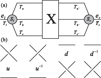
A 3-strand braid, formed by the three common edges of two adjacent nodes, is in fact an equivalence class of diffeomorphic local sub networks of the whole framed spin network embedded in a topological 3-manifold. We study a braid through its 2-dimensional projection, called a braid diagram. We therefore will not distinguish braids from braid diagrams unless an ambiguity arises. A generic example of such a braid diagram is depicted in Fig. 1(a). Although the properties of a braid should not depend on which representative is chosen for the equivalence class, in some cases an appropriate representative makes things easier.
In [5] our choice was to represent an equivalence class by a braid diagram which has zero external twists. This simplifies the interaction condition and the graphic calculus developed in [4, 5]. Each class has one and only one such representative. Thus a braid represented this way is said to be in its unique representation. This representation is important because according to [7], each multiplet of actively interacting braids under the discrete transformations, which are analogous to the C, P, and T in particle physics, found in [7] is uniquely characterized by a non-negative integer, viz the number of crossings of the braids in their unique representations in the multiplet. In this paper we will use the unique representation exclusively.
Along with the graphic calculus, an algebraic notation and the corresponding calculational method of braid interactions were put forward in [6, 7]. This algebraic formalism plays a key role in finding the conserved quantities of braids and the discrete transformations mapped to C, P, T, and their combinations, in [6, 7, 8]. We will use both the graphic and algebraic calculus in this paper. Thus let us briefly review the algebraic notation.
The generic braid shown in Fig. 1(a) is denoted by
where the crossing sequence is an element of the braid group , and the twists, , , etc, take values in . A crossing sequence is generated by the four generators shown in Fig. 1(b), and can then be written as with . It is useful to define the quantity for [8]. So clearly , meaning no crossing. The generators are assigned integral values according to their handedness, namely and . Therefore, crossings of a braid can also be summed over to obtain an integer, the crossing number: , of the braid, where is the number of crossings.
The of a braid induces a permutation , an element in the permutation group , of the three strands of the braid. The triple of internal twists on the left of and the one of the right of are thus related by and . That is, is a left-acting function of the triple of internal twists, while its inverse, is right-acting. The inverse relation between and is understood as:
| (1) |
Note that the twists such as and are abstract and have no concrete meaning until their values and positions in a triple are fixed. Thus, means , etc, and . Note also that the in the out most layer in the notation should be kept formal rather than an explicit element in because the is needed to record the crossing sequence. For example, if we obtain a braid, say in some process, then while we can write the as to complete the addition in the parenthesis, we should keep as it is but not explicitly as . The relation between and its inverse suggests that a generic braid can be equally denoted by
Given this notation, we express a braid in its unique representation as
or simply , dropping out the zero’s.
We have shown the algebraic structure of the set of all stable 3-strand braids in [7] under the braid interaction found in [5]. Hence, we choose to denote the set of stable braids by . However, for reasons which will become transparent in the sequel we should enlarge by adding two more braids:
| (2) |
which are completely trivial22 2 It is highly important to note again that at this point spin network labels have not been taken into account yet. When spin network labels are rather considered there are two immediate consequences. 1) are not just two braids, but infinite number of braids because they can be colored by different sets of spin network labels, so is any other braid in . 2) are only trivial topologically but not algebraically and neither physically.. are actually unstable according to [5] because they are dual to a 3-ball. If we tolerate their instability they are obviously actively interacting. Bearing this in mind, let us still call the enlarged set the set of stable braids but use as its notation. According to [5], can be divided into the disjoint union of three subsets: the subset of all actively interacting braids (including ), the subset of all propagating braids which are do not actively interact, and the subset of stationary braids which are passive in all interactions and do not propagate; they are denoted respectively by , , and . Therefore, we have
| (3) |
Moreover, the set of propagating-only braids can be further divided as
| (4) |
where denotes the subset of braids which only propagate to the left, is the subset of braids which only propagate to the right, and contains two-way propagating braids.
Because a new type of interaction will be introduced in this paper, to get rid of any possible confusion we call the interaction introduced in [5] the direct interaction and notate it by , while name the new interaction exchange interaction for reasons will be clear when it is defined, denoted as . As a consequence, a bare sign between two braids only means the adjacency of the braids. As pointed out in [7], is closed under the direct interaction, i.e. .
This will help to make the algebraic structure of braids and the contact of our model with particle physics clearer.
3 Exchange interaction
[5] has shown that two neighboring braids may interact and merge into a new braid. This process is called direct interaction. One of the two braids in a direct interaction must be an actively interacting braid. That is, we only have the following possible direct interactions: , . Fortunately, there exists, as we are to show, another type of interaction, namely the exchange interaction, which can take two adjacent braids in to another two neighboring ones in the same set. In fact, exchange interaction can be defined on the whole as a map, . It will be clear shortly that there is always an exchange of a virtual actively interacting braid in an exchange interaction, giving why exchange interaction is so christened. It is useful to keep track of the direction of the exchange of the actively interacting braid during an exchange interaction. Therefore, we differentiate a left and a right exchange interaction, respectively denoted by and . The arrow indicates the ”flow” of the virtual actively interacting braid.
The graphic definition of right exchange interaction is illustrated in Fig. 2. The left one can be defined likewise. We now explain with the help of our algebraic notation the process in detail as follows.
- 1.
We begin with the two adjacent braids, in Fig. 2(a). Their algebraic forms are: and . ’s right end-node and ’s left end-node are set in the same state, , to satisfy the interaction condition[5]. We also assume that is right-reducible (not necessarily fully right-reducible), such that the crossing sequence of has a maximal reducible segment, say , as shown in the figure. The reason for this will be clear soon. (Similarly, for left exchange interaction one should have left-reducible. If is right-reducible and is left-reducible, both left and right exchange interactions may occur but they lead to different results in general.)
- 2.
A move on the two nodes in the state now leads to Fig. 2(b). The dashed lines simply means the crossing relation between the green lines and black ones can not be determined unless we know what exactly the state is.
- 3.
Because is the reducible part of the crossing sequence of , according to [5] one can translate the three new nodes - one in state and two in - in (b) along with the edges , and to the left of , and rearrange them by equivalence moves defined in [4] in a proper configuration ready for a move, as seen in Fig. 2(c). This is why we assume is
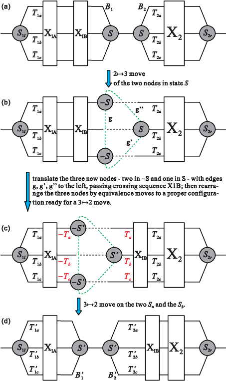
Figure 2: Definition of right exchange interaction: , . In (b), the dashed lines emphasize the dependence of the move on the state of the two nodes on which the move is taken. In (c) and (d), . In (c), the dashed line means that the configuration depends on . In (d), and are the internal twists of and respectively, which are explained in the text. right-reducible; otherwise, the translation is not viable. Due to [5], in Fig. 2(c) the three nodes are shuffled by the translation and their states are related to by . However, because is arbitrary dashed lines are also used in Fig. 2(c) for undetermined crossing relation between the green edges and the black ones. This procedure introduces twists in pair on the strands: and , labeled in red in Fig. 2(c).
Note that the triples and are not existing on the strands separately. One should add to with the permutation induced by taken into account, i.e. . The relation between and is likewise. This cannot be represented in the figure, which is a limitation of the graphic notation.
- 4.
We then perform the move and arrive at Fig. 2 (c) which shows two new adjacent braids, and , related to and by
(5) (6) This completes the right exchange interaction, .

It can be shown, according to [5, 7], that the only possible triple in Fig. 2(c) is exactly the same as the triple of internal twists of the actively interacting braid, , in Fig. 3. Note that as proved in [6], for an actively interacting braid of the form in Fig. 3, . Hence, ’s left and right end-nodes are respectively in the same states as that of the left end-node of in Fig. 2(d) and that of the right end-node of in Fig. 2(a). Thus the form of braid in Fig. 2(d) due to the final move in the interacting process must be precisely the result of the direct interaction of and . That is, by [7] we have
which validates the relation in Eq. 6.
Therefore, the process of the right exchange interaction defined by Fig. 2 is like that gives out the actively interacting braid in Fig. 3 which is then combined with by a direct interaction. In other words, and interact with each other by exchanging a virtual actively interacting braid , and become and . Or one may say that an exchange interaction is mediated by an actively interacting braid. This implies an analogy between actively interacting braids and bosons33 3 More generally, this should imply the analogy between actively interacting braids and particles that mediate interactions, which should potentially include super partners of gauge bosons.. Note that in an exchange interaction, there does not exist an intermediate state in which only the virtual actively interacting braid is present because our definition of a braid requires the presence of its two end-nodes.
The above can be summarized by the following theorem as the first main result of the paper. (The case of left exchange interaction is similar.)
Theorem 1.
Given two adjacent braids, , is on the left and is right-reducible with the reducible segment of its crossing sequence, and , there exists a braid , with , such that it mediates the exchange interaction of and to create , i.e.
| (7) | ||||
It is important to remark that the reducibility of either braid in an exchange interaction is not necessary if we have included braid in Eq. 2. For example, for two neighboring irreducible braids one can still have the steps in Fig. 2(a) and (b), then skip over Fig. 2(c) because there are no reducible crossing segment to be translated through, and directly take the step in Fig. 2(d). Such a procedure is still dynamical because of the action of evolution moves and thus can be considered a special case of exchange interaction. Needless to say, the actively interacting braid being exchanged in such an interaction is one of the two trivial braids . This ensures that exchange interaction is a map on .
Another important remark is that two braids can have exchange interactions in different ways, in contrary to direct interaction. The occurrence of an exchange interaction on two braids does not have to exhaust the maximal reducible crossing segment of the reducible braid. For example as in Fig. 2, since is the maximal reducible crossing segment, we may take it to be the concatenation of two reducible crossing segments, i.e. , then the translation taking Fig. 2(b) to (c) is allowed to terminate after passing through which becomes the crossing sequence of the virtual actively interacting braid in this new process. This certainly leads to two braids different from those in Fig. 2(d). In an ideal scenario, each possible way of the exchange interaction of two braids should have certain probability to occur.
There is an analogy of this in particle physics. Since quarks have both electric and color charges, both photons and gluons can mediate forces on quarks. However, the relation between actively interacting braids and bosons is yet not an actual identification. In fact, if each actively interacting braid corresponded to a boson, there would be too many ”bosons”. The underlining physics of that two braids can have exchange interactions in different ways deserves further studies.
It should be emphasized that each individual exchange interaction is a process giving rise to a unique result44 4 With spin network labels the result is not unique any more because two topologically equal braids can be decorated by different sets of labels, and an interaction should result in a superposition of braids labeled differently.. For preciseness, an expression like is only formal. Only when the exact forms of and , in which their reducible segments are explicitly present, are given, acquires a precise and unique meaning. In computing an exchange interaction, we have to specify explicitly our choice of the reducible crossing segment of the braid which gives out the virtual actively interacting braid which depends on this choice. For any such choice Theorem 1 holds.
[5, 6, 7] have shown that there are two representative-independent conserved quantities of stable braids, namely the effective twist and the effective state , the former of which is additively conserved under direct interaction while the latter is multiplicatively conserved. Due to the representative-independence of these two quantities, we can write down their expressions for an arbitrary braid in its unique representation, say , as and . These two quantities are important. [8] has shown that or certain function of of a braid can be accounted for the ”electric” charge of the braid. That is, braids can be charged. On the other hand, for actively interacting braids is a characteristic quantity because for any such braid. The following theorem presents that exchange interaction also preserves these two quantities in the same way as direct interaction does.
Theorem 2.
Given two neighboring stable braids, , such that an exchange interaction (left or right or both) on them is doable, i.e. , , the effective twist is an additive conserved quantity, while the effective state is a multiplicative conserved quantity, namely
| (8) | ||||
This conservation law is independent of the virtual actively interacting braid being exchanged during the exchange interaction.
Proof.
It is sufficient to prove this in the case of right exchange interaction, the other cases follow similarly. One can assume and are in the form as they are in Theorem 1. Hence, according to Theorem 1 one can readily write down
where , and
Hence we have the following:
where the use of , , and has been made. ∎
Therefore, exchanges of actively interacting braids give rise to interactions between braids which are charged under the topological conservation rules. The conservation of is analogous to the charge conservation in particle physics.
3.1 Asymmetry of exchange interaction
As in the case of direct interaction[7], exchange interaction is not symmetric either. The asymmetry of exchange interaction is two-fold. On the one hand, given , which are both right-reducible (left-reducible), in general (). This is henceforth called the asymmetry of the first kind. On the other hand, if and are respectively right- and left-reducible, then in general , which is christened the asymmetry of the second kind. Most probably, the interactions on either side of these inequalities simply does not occur due to the interaction condition. Even when these interactions do occur, the inequalities hold in general. However, we now show that there are cases where exchange interaction can be symmetric.
An issue is that two braids may have several different exchange interactions. It is then impossible for, say , to be equal to for all possible ways of how and may interact. The only precise question we can answer is actually, taking right exchange interaction as an example: For any and , among all possible ways of and , does there exist a way in which the reducible crossing segments of and are chosen, such that in this way ?
We first study the the asymmetry of the first kind. It suffices to check the right exchange interaction and the left one follows likewise. We assume and , with and certain choices of the reducible crossing segments of respectively and . The fact that both and are assumed to be legal requires that and for some and . Hence, we have and . With this, Theorem 1 immediately gives us
where and ; and are the triples of internal twists of the two virtual actively interacting braids being exchanged in the two interactions respectively. Requiring that the RHS of the two interaction equations are equal term by term gives rise to
| (9) |
and
| (10) |
Eq. 9 also implies . We can then rewrite as , as , and both and as . As a result, the two triples and must be equal, which is understood by recalling the steps in Fig. 2. Thus Eq. 10 becomes
whose only solution is
Therefore, and must be exactly the same. By the same token, this should be true for the case of left exchange interaction too.
We now investigate the asymmetry of the second kind. We assume a right-reducible braid with the choice of its reducible crossing segment, and with the choice of its reducible crossing segment. Note that the right end-node of has already been made the same as the left end-node of such that and are both allowed.
By Theorem 1 we get
where , and the triple of internal twists of the virtual actively interacting braid in the interaction. Analogously we also have
where , and the triple of internal twists of the virtual actively interacting braid in the interaction. The term-by-term equality of the RHS of the above two equations now helps us to pin down the conditions on and . Firstly, we must have which requires and keeping . Secondly, we demand and . The only solution of this is readily . Or equivalently, we obtain . This sets and hence guarantees . These results now turn the constraint on the triples of internal twists of and to be
| (11) |
Surprisingly, Eq. 11 actually puts no more constraint on and because it is automatically satisfied. The reason is as follows.
In both cases, namely and , the configurations obtained by the first move are the same, which has three new nodes and three new edges (like the dashed green ones in Fig. 2(b)). We call this configuration, . In the case of , one needs to translate the to the left, passing through , then rearrange by equivalence moves into another configuration, say , which is a proper for a move. The equivalence moves taking to equips with two opposite triples of twists, viz on the left of and on the right. is the very triple of internal twists of the virtual actively interacting braid exchanged by and in this interaction. In the case of , one translates to the right, passing the crossing sequence , and reforms it by equivalence moves into another one, say , which is also ready for a move. Likewise, is equipped with on its left and on its right. is the very triple of internal twists of the virtual actively interacting braid exchanged in the process of . Nevertheless, because of , according to [8], and happen to be related to each other by a discrete transformation which is considered as a transformation. By the action property of a (see [8] for details), we have precisely
| (12) |
Putting this aside first, we have another useful identity from [8]55 5 The equation A.2 in the reference:
where stands for an arbitrary triple of internal twists, and , the reversion operation of a crossing sequence. [8] also defines the inversion of a crossing sequence, namely . Obviously, . However, regarding the permutation induced by a crossing sequence, [8], which then means . Consequently, the equation above is extended to
| (13) |
Finally, in view of Eqs. 12 and 13, and all the relations we have in hand, it is easy to see that Eq. 11 is satisfied. That is, the triples of internal twists of and can be any thing they can. Therefore, for and can be equal in certain way, we demand and . For compactness, the discussion above is concluded by the following theorem.
Theorem 3.
Exchange interaction between two arbitrary braids , if allowed, is asymmetric in general. The asymmetry of the first kind goes like, (), whereas the asymmetry of the second kind reads . However, there exist the following special cases.
- 1.
For that there exists a way in which (), and must be in the form
(14) where represents an arbitrary triple of internal twists, and is the chosen reducible crossing segment.
- 2.
For that there exists a way in which , and have to be like
(15) where and are the specified reducible crossing segments of and respectively during the two interactions.
The existence of exchange interaction brings the braids and their dynamics closer to Quantum Field Theory. This is not to say that we already have a fundamental field theoretic formulation of our theory. Rather, we can have an effective field theory describing the dynamics of braids. To make this more transparent, we need first to show another dynamical process of braids.
4 Braid Decay
It is implied in [5] that there can be reversed processes of direct interactions: a braid may split into two braids.
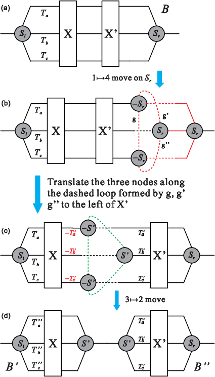
We may call a reversed direct interaction a decay. Hence, obviously through decay a braid always radiates at least one actively interacting braid. In a direct interaction, the actively interacting braid involved may interact with the other braid from the left or from the right. As a result, via a decay the braid may radiate an actively interacting braid to its right or to its left, depending on whether the braid is right-reducible or left-reducible. We thus differentiate a left-decay from a right-decay. The former is symbolized by , indicating that , while the latter is denoted by for that .
Fig. 4 presents the defining process of right-decay. Fig. 4(a) shows a right-reducible braid, , with a chosen reducible crossing segment . As in an exchange interaction can be a part of the maximal reducible crossing segment of ’. This indicates that generically a braid can also have different ways of decay, corresponding to each choice of the reducible segment. We thus need to specify this choice in a specific decay process.
Taking a move on the right end-node of leads to Fig. 4(b). One then translate the three nodes, one in state and two in , along the red dashed loop in Fig. 4(b) to the left of , and rearrange them in a proper configuration for a move, as shown in Fig. 4(c). This produces the pair of opposite triples of twists in Fig. 4(c), namely and . Note that the triple , which is in red, should be understood to be added to , the original triple of internal twists of , taking into account the permutation induced by , i.e. . Finally, a move results in Fig. 4(d) which depicts the two resulted adjacent braids, and . Thus we have
| (16) |
where and . Left-decay is defined similarly.
By the same logic as that of the remark below Theorem 1, an irreducible braid can also decay but it only radiates a completely trivial braid which is either or in Eq. 2. An irreducible braid hence stays unchanged topologically under a decay.
The notation of decay already implies that a decay is in general not symmetric. For a braid which is able to decay in both directions, say and , there is no way for and because we must have but . Even if is an actively interacting braid, its left and right decays give rise to different results because both of its left and right decays have more than one ways to occur, as pointed out above. There are also special cases in which an actively interacting braid has a certain left decay that is the same as a certain right decay of it. The conditions of this are similar to those for a direct interaction to be symmetric found in [7].
On the other hand, a direct interaction is not guaranteed to have a corresponding decay despite that a decay can be viewed as the reverse of certain direct interaction. This is because pair cancelation of crossings may occur in a direct interaction and in [7] it is pointed out that in the definition of a 3-strand braid the crossing sequence of the braid in any representation is the shortest one among all equivalent ones due to braid relations. Indeed, one can easily show that a braid in cannot decay into a braid in , although a direct interaction in the opposite direction is always possible.
Because of the relation between decay and direct interaction, effective twist and effective state must be respectively an additive conserved quantity and a multiplicative conserved quantity under a decay. By the same token, because direct interactions are invariant under C, P, T, and their combinations[8], so are decays. Decay and direct interaction of braids indicate that an actively interacting braid can be singly created and destroyed. This reinforces the implication that actively interacting braids are analogous to bosons.
5 Braid Feynman diagrams
Our study of braid excitations of embedded framed spin networks, in particular the discovery of the dynamics of these excitations, namely direct and exchange interactions, and decay of braids, makes it possible to describe the dynamics of braids by an effective theory based on Feynman diagrams. These diagrams are called braid Feynman diagrams. We remark that as a distinction from the usual QFT Feynman diagrams which do not have any internal structure, each braid Feynman diagram is an effective description of the whole dynamical process of an interaction of braids, its internal structure records how the braids and their neighborhood evolve.
We use ![[Uncaptioned image]](0809.4464v2/outProp.png) and
and ![[Uncaptioned image]](0809.4464v2/inProp.png) for respectively outgoing and ingoing
propagating braids in ,
for respectively outgoing and ingoing
propagating braids in ,
![[Uncaptioned image]](0809.4464v2/outStat.png) and
and
![[Uncaptioned image]](0809.4464v2/inStat.png) for
respectively outgoing and ingoing stationary
braids66
6
Stationary braids although are not directly
propagating on the spin network it resides, may still be able to
move around under the change of its surroundings due to the network
evolution, and may also propagate physically in the continuum limit
of the theory. in . Because it is implied that
actively interacting braids are analogous to bosons, outgoing and
ingoing braids in are better represented by
for
respectively outgoing and ingoing stationary
braids66
6
Stationary braids although are not directly
propagating on the spin network it resides, may still be able to
move around under the change of its surroundings due to the network
evolution, and may also propagate physically in the continuum limit
of the theory. in . Because it is implied that
actively interacting braids are analogous to bosons, outgoing and
ingoing braids in are better represented by
![[Uncaptioned image]](0809.4464v2/outAct.png) and
and
![[Uncaptioned image]](0809.4464v2/inAct.png) respectively.
respectively.
In accordance with left and right decay, we will henceforth denote left and right direct interactions by and respectively. Note that if the two braids being interacting are both actively interacting, the direction of the direct interaction is irrelevant because the result does not depend on which of the two braids plays the actual active role in the interaction[5, 6]. According to the algebraic structure of braids under direct interaction found in [7]77 7 See Theorem 4 in the reference., namely and , the only possible single vertices of right direct interactions are listed below. (Those corresponding to left direct interactions are left-right mirror images these.)


Similarly, right decay have the possible basic single vertices in Fig. 6. (The left-decay vertices are left-right mirror images of these.) In the second figure of Fig. 6 when is irreducible, should be understood equal to and is either of the two braids in Eq. 2.
The arrows over the wavy lines in Figs. 5 and 6 are important for that they differentiate a left process from a right process. More importantly, they encode the fact that the correspondence between decay and direct interaction is not one-to-one and can be used to see which kind of direct interactions can have a corresponding decay. That said, one can flip the arrow over the braid in each of the first three diagrams in Fig. 6 and obtain the diagram of the corresponding left direction interaction. One can also turn the fourth diagram in Fig. 6 upside down to get its corresponding direct interaction diagram. However, for example, one cannot flip the arrow over the wavy line in the fourth diagram in Fig. 5 to obtain a decay of the braid in the diagram because there does not exist such a left decay according to the mirror images of the diagrams in Fig. 6.

The result of an exchange interaction of two braids, say by exchanging some virtual , is the same as that of the combined process of the decay, , and the direct interaction . However, it is important to note that the former process and the latter combined process are two topologically and dynamically distinct processes; they only have the same in and out states topologically. Therefore, we obtain in Fig. 7 all possible basic 2-vertex diagrams for right exchange interaction.
The left-right mirror images of the diagrams in Fig. 7 are certainly the basic diagrams for left exchange interaction. In Fig. 7(e), (f), (h), (n), (s) and their left-right mirror images, if happens to be irreducible, and or are understood. Given all these it becomes manifest that exchange interaction is invariant under the C, P, T and their products defined in [8], as in the case of direct interaction and decay.
Recalling Theorem 3, braid Feynman diagrams make it transparent to tell whether an exchange interaction can be symmetric. Regarding the asymmetry of the first kind, one simply needs to check if the diagram of an interaction looks the same as its left-right mirror with also the arrow over the virtual braid reversed. Fig. 7(c), (d), (h) through (o), and (q) through (t) depict exchange interactions which do not allow any violation of the asymmetry of the first kind, viz . The reason is that in each of these diagrams, the out-state contains two braids in two different divisions respectively. Their mirror images have the same kind of asymmetry with respect to left exchange interaction.
As to the asymmetry of the second kind, one should check if the arrow over the virtual braid in a diagram can be flipped. According to this, the four diagrams in Fig. 7(q) through (t) respect the asymmetry of the second kind, i.e. in any case, because the arrow over the braid in any of these diagrams cannot be flipped, for which the fact that a stationary braid does not decay into a propagating braid is accounted. Therefore, the exchange interactions respectively in Fig. 7(q) to (t) are completely asymmetric.
Nevertheless, interactions respectively in Fig. 7(a) through (p) can have instances violating the asymmetry of the second kind if conditions in Theorem 3 are satisfied, because these diagrams are symmetric under flipping the arrow over the braid in each of them. As a result, the exchange interactions which can be fully symmetric when conditions in Theorem 3 are satisfied correspond respectively to the diagrams in Fig. 7(a), (b), (e), (f), (g), and (p).
The analogy between actively interacting braids and bosons is manifested by the braid Feynman diagrams in Figs. 5, 6, and 7. Fermionic degrees of freedom may correspond to those braids which are not actively interacting because their interactions are mediated by the actively interacting ones. They are more probably corresponding to braids in , which are chiral propagating but not actively interacting.
More complicated braid Feynman diagrams including the loop ones can be constructed out of these basic vertices. As a result, there should exist an effective field theory based on these diagrams, in which the probability amplitudes of each diagram can be computed. For this one should figure out the terms evaluating external lines, vertices, and propagators of braids.
In a more complete sense, one may try to write down an action of the effective fields representing braids that can generate these braid Feynman diagrams. In such an effective theory, each line of a braid Feynman diagram represents an effective field characterizing a braid; it should be labeled by characterizing quantities of the braid represented by the line, which are elements of certain groups or the corresponding representations of these groups. For a braid these quantities are its two end-node states which are elements of , its crossing sequence, an element of the braid group , its twists which are elements in , and spin network labels when they are taken into account. Moreover, there are constraints of these group elements on the lines meeting at a vertex.
This is more difficult than just to find a way to compute the probability amplitude of each braid Feynman diagram. In any case, the very first challenge of fulfilling this task is to choose an appropriate mathematical language. In the next section we will briefly mention three possible formalisms.
However, these braid Feynman diagrams put a constraint on defining the probability amplitudes regardless of the underlining mathematical language. We use an example to illustrate this point. Let us consider the braid Feynman diagram in Fig. 7(a) for some specific interaction. This diagram is the same as concatenating the first diagram in Fig. 6 with the first diagram in Fig. 5 from the left along the wavy line. That is, the exchange interaction, by exchanging some virtual , and the combined process of the decay, , and the direct interaction , have identical in and out braid states at this tree level. We hence expect the following equality at this level, which is only formal,
| (17) |
The LHS of Eq. 17 is the probability amplitude of the exchange interaction, which is independent of the virtual braid being exchanged during the interaction but only determined by the evolution moves involved in the interaction and the external lines in Fig. 7(a), namely , , and . The first term on the RHS of this equation is the conditional probability amplitude of the direct interaction provided with the occurrence of the decay and the meeting of and . Besides , , , and the corresponding evolution moves, this also certainly depends on the braid which is characterized by a set of parameters, denoted by , including the end-node states, spin network labels, twists, and crossings of . The second term on the RHS, i.e. represents the propagator (however it will be defined) of , which is obviously also a function of . must be summed over due to the independence of the final result on . There are analogies of this summation in usual quantum field theories, e.g. the integration over the momentum defining the propagator of the virtual particle in an interaction, and the summation over polarizations of gauge bosons.
Eq. 17 is generic though is derived with the help of a specific example because one can simply replace the exchange interaction on the LHS with any other one and substitute the corresponding direct interaction and decay on the RHS simultaneously. No matter how the continuum limit of our theory is to be obtained, the momentum of the braid in this limit should be accounted for by . Therefore, Eq. 17 can be used for a validity check of the theory’s future possible developments which will be able to define the probability amplitudes of the dynamical processes of our braids.
6 Conclusions and future work
In conclusion, we have found the exchange interaction of braids, which has two kinds of asymmetry. Conserved quantities under exchange interaction are discussed. We also discussed decay of braids. The existence of exchange interaction and its relation with direct interaction and decay of braids imply the analogy between actively interacting braids and bosons. Braid Feynman diagrams are developed and used to represent the dynamics of braids. An effective theory describing braid dynamics can be based on these braid Feynman diagrams. We emphasize that an interaction of two braids is not point-like, although braid Feynman vertices are point-like. This is similar to the case of String Theory in which two strings do no interact at a point.
Despite the lack of a fully fundamental theory of quantum gravity with matter, an effective theory of topological excitations, such as our braids, of quantum geometry may be more relevant to the testable region of our physical world. The study of collective modes in condensed matter physics provides a great motivation to this. For example, in the current stage of the string-net condensation, all Standard Model gauge fields and fermionic fields but chiral fermions appear to be low energy effective fields emergent out of certain high energy lattice models[14].
Our next step is to compute the probability amplitudes of the braid Feynman diagrams and to write down the effective field theory of these braid excitations in an algebraic way. To compute the probability amplitudes, one may adopt the methods in some spin foam models, in which the probability amplitude of each evolution move is most basic. However, the way to define the probability amplitude of an evolution move in our situation should be modified because all current spin foam models are unembedded but our spin networks are embedded in a topological 3-manifold, which means that not only spin network labels but also the topological quantities defining the braids should be considered.
One may also borrow the ideas from Group Field Theories in which a field is a scalar function of group elements defining a fundamental building block of spacetime[16]. We can try to construct a group field theory of braids, in which a field is a function of the group elements defining a braid. The interacting term in this theory can be written done with the help of braid Feynman diagrams. The very first challenge is to construct the field representing a braid. As a first step, one may start with a toy model, considering actively interacting braids only, or even merely certain actively interacting braids, of a spin network. This is what we are currently working on.
The third possibility is by means of tensor categories. The motivations of adopting tensor categorical methods have been discussed in [8]. The connection between LQG and Spin Foam Models and Tensor Categories has actually been realized for about two decades. It was first introduced by Crane[17] and elaborated by others, e.g. Kauffman[18]. One should also note that the string network condensation by Wen et al[14] and their newly proposed tensor-net approach[15] are examples of approaches of unifying gravity and matter which indicate that tensor category might be a correct underlying mathematical language towards this goal. This formulation would be purely algebraically, referring to any topological embedding is no longer needed.
Another open issue is that we cannot justify for now whether the actively interacting braids are analogous to bosons or gauge bosons in particular. For the latter to be true, actively interacting braids should obey certain gauge symmetry. We would like to see gauge symmetries arise when we include spin network labels, which are normally gauge group representations, in our model. The three possible approaches introduced above may have an answer for this question.
Acknowledgements
The author thanks Sundance Bilson-Thompson, Jonathan Hackett, and Matthias Wapler for helpful discussions. His gratitude also goes to Daniele Oriti and Florian Conrady for clarifying some GFT concepts. He appreciates Zhengcheng Gu for discussions on tensor categories and the clarification of Wen’s work. He is grateful to Song He and Lee Smolin, his advisor, for invaluable comments on the manuscript. Research at Perimeter Institute for Theoretical Physics is supported in part by the Government of Canada through NSERC and by the Province of Ontario through MRI.
References
- [1] S. Bilson-Thompson, F. Markopoulou, L. Smolin, Quantum gravity and the standard model, Class. Quant. Grav., 24, 3975 (2007), hep-th/0603022.
- [2] J. Hackett, Locality and Translations in Braided Ribbon Networks, hep-th/0702198.
- [3] S. Bilson-Thompson, J. Hackett, and L. Kaufmann, Particle Identifications from Symmetries of Braided Ribbon Network Invariants, arXiv:0804.0037.
- [4] Y. Wan, On Braid Excitations in Quantum Gravity, arXiv:0710.1312.
- [5] L. Smolin, Y. Wan, Propagation and Interaction of chiral states in quantum gravity, Nucl. Phys. B, 796, 331 (2008).
- [6] J. Hackett, Y. Wan, Conserved Quantities for Interacting Four Valent Braids in Quantum Gravity, arXiv:0803.3203.
- [7] S. He, Y. Wan, Conserved Quantities and the algebra of Braid excitations in Quantum Gravity, Nucl. Phys. B 804, 286 (2008), arXiv:0805.0453.
- [8] S. He, Y. Wan, C, P, and T of braid excitations in quantum gravity, Nucl. Phys. B 805, 1 (2008), arXiv:0805.1265.
- [9] F. Markopoulou, I. Premont-Schwarz, Conserved Topological Defects in Non-Embedded Graphs in Quantum Gravity, Class. Quant. Grav. 25, 5015 (2008), arXiv:0805.3175.
- [10] S. Bilson-Thompson, A topological model of composite preons, hep-ph/0503213.
- [11] D. W. Kribs, F. Markopoulou, Geometry from quantum particles, gr-qc/0510052. F. Markopoulou and D.Poulin, Noiseless subsystems and the low energy limit of spin foam models, unpublished.
- [12] C. Rovelli, Loop Quantum Gravity, Living Rev.Rel. 1 (1998) 1, gr-qc/9710008; Quantum Gravity, Cambridge University Press, 2004. D. Oriti, Spin Foam Models of Quantum Spacetime, Ph.D. Thesis, arXiv: gr-qc/0311066. A. Perez, Spin Foam Models for Quantum Gravity, Class. Quant. Grav. 20 (2003) R43, arXiv:gr-qc/0301113. J. Baez, An Introduction to Spin Foam Models of Quantum Gravity and BF Theory, Lect. Notes Phys. 543 (2000) 25, arXiv:gr-qc/9905087.
- [13] R. Penrose, Angular monentum: an approach to combinatorial space-time, Quantum Theory and Beyond, Cambridge University Press, 1971; On the nature of quantum geometry, Magic without magic, Freeman, San Francisco, 1972.
- [14] M. A. Levin, X. Wen, String net condensation: A Physical mechanism for topological phases, Phys. Rev. B, 71:045110 (2005); A Unification of light and electrons based on spin models, cond-mat/0407140.
- [15] Z. Gu, M. A. Levin, X. Wen, Tensor-entanglement renormalization group approach to topological phases, arXiv:0807.2010.
- [16] D. Oriti, The group field theory approach to quantum gravity, arXiv:gr-qc/060703v2.
- [17] L. Crane, 2-D physics and 3-D topology, Commun. Math. Phys. 135:615 (1991).
- [18] L. Kauffman, Knots and physics, World Scientific.