Flow Equation for Supersymmetric Quantum Mechanics

Franziska Synatschke Georg Bergner Holger Gies Andreas Wipf Affiliation: Theoretisch-Physikalisches Institut, Friedrich-Schiller-Universität Jena, Max-Wien-Platz 1, D-07743 Jena, Germany Email: franziska.synatschke@uni-jena.de, g.bergner@tpi.uni-jena.de, gies@tpi.uni-jena.de, wipf@tpi.uni-jena.de Affiliation: E-mail:

Abstract:

We study supersymmetric quantum mechanics with the functional RG formulated in terms of an exact and manifestly off-shell supersymmetric flow equation for the effective action. We solve the flow equation nonperturbatively in a systematic super-covariant derivative expansion and concentrate on systems with unbroken supersymmetry. Already at next-to-leading order, the energy of the first excited state for convex potentials is accurately determined within a 1% error for a wide range of couplings including deeply nonperturbative regimes.

Keywords:

Renormalization Group, Superspaces, Supersymmetric Effective Theories, Nonperturbative Effects

1 Introduction

Supersymmetry is a key ingredient in the construction of models of fundamental physics, since it provides for a salient possibility to combine internal symmetries with the Poincare group. Even though distinguishing features of supersymmetric systems can be understood within perturbation theory, many important properties such as collective condensation phenomena often related to symmetry breaking are inherently nonperturbative. If supersymmetry is realized in nature, powerful and flexible nonperturbative tools will be needed to investigate the underlying mechanisms of these strong-coupling phenomena.

As supersymmetry does not only mix bosons and fermions but also involves spacetime translations, lattice methods built on spacetime discretization often go along with a partial loss of supersymmetry. The construction of appropriate lattice formulations in addition to the challenge of dealing with dynamical fermions is an ongoing effort [1, 2, 3, 4]. These studies need to be complemented by nonperturbative continuum methods preferably with manifest supersymmetry.

In recent years, the functional renormalization group (RG) has become such a nonperturbative tool as has been demonstrated by many successful applications ranging from critical phenomena, via fermionic systems and gauge theories even to quantum gravity, see [5, 6, 7, 8, 9, 10] for reviews. However, the number of applications to supersymmetric systems is rather small. In this work, we formulate and test the functional RG for a simple supersymmetric system, namely, supersymmetric quantum mechanics.

In fact, ordinary quantum mechanics has often been used for illustrating and testing the nonperturbative capabilities of the functional RG, since the RG flow equations are easily obtained and approximate solutions can directly be compared to known exact results or high-precision numerics. In particular, the study of ground- and excited-state energies with RG techniques has received a great deal of interest in the last few years [11, 12, 13, 14, 9]. Whereas single-well potentials can be treated comparatively easily even at extreme coupling, double-well potentials have turned out to be more challenging, since the analytic RG flow equations have to build up the non-analyticities from tunneling; the latter are usually described in terms of instantons, being of topological nature.

In [11], Horikoshi et al. study the quantum double well using an expansion in powers of the field, [12] and [14, 15] go beyond this approximation and solve the RG flow in the so-called local-potential approximation for the effective potential (i.e., leading-order derivative expansion). Within the propertime RG, Zappalà [13] also includes wave function renormalization (i.e., next-to-leading-order derivative expansion), and finds good agreement for the mass gap. Particularly, this study convincingly demonstrates that the functional RG automatically includes also fluctuations of topological degrees of freedom without explicitly introducing them by hand.

Supersymmetric quantum mechanics was introduced by Witten [16] as a toy model for spontaneous symmetry breaking. The first to use renormalization group methods for supersymmetric quantum mechanics were Horikoshi et al. [11]. They investigated a broken supersymmetric model with nonperturbative renormalization group methods and calculated the nonvanishing ground-state energy and that of the first excited state in a polynomial expansion of the effective potential. They found good agreement with the exact results for all cases where tunneling is not important. This latter region has been covered in [15] within the propertime RG, where again the observation was made that a wave function renormalization improves the results for the energy spectrum, i.e., helps including tunneling.

Both approaches use regulators that break supersymmetry which makes it difficult to distinguish between explicit and spontaneous or dynamical supersymmetry breaking. One possibility to solve this problem is the inclusion of symmetry breaking by the regulator into the symmetry relations as done in [17, 18]. In fact even the lattice discretisation can be viewed as a supersymmetry breaking regulator. The corresponding modified symmetry relations are similar to the Ginsparg-Wilson-relation, introduced in [19] and extended in [20], and were established for supersymmetric models in [21]. But so far a solution of these relations is possible only in some simple cases. In this paper, we present an approach to flow equations for supersymmetric quantum mechanics which maintains supersymmetry manifestly on the level of the RG flow equation with the aid of an invariant regulator. In contrast to [11] and [15], we concentrate on a system with unbroken supersymmetry.

Our approach is similar to the works by Bonini and Vian [22, 23] where a supersymmetric regulator for the $4d$ Wess-Zumino model is presented. The functional RG has also been formulated for supersymmetric Yang-Mills theory in [24] employing the superfield formalism; for applications, see also [25, 26]. Very recently, Rosten has investigated general theories of a scalar superfield including the Wess-Zumino model with the aid of a Polchinski-type of RG equation with elegant applications in the context of non-renormalization theorems [27]. A construction of a Wilsonian effective action for the Wess-Zumino model by perturbatively iterating the functional RG has been performed in [28].

The paper is organized as follows: in Sect. 2, we briefly recall the basics of Euclidean supersymmetric quantum mechanics, also introducing our notation. In Sect. 3 we derive the flow equation for the superpotential and introduce a general class of supersymmetric regulator functions. In Sect. 4 we discuss the flow equation for the superpotential for different regulators. In Sect. 5 we introduce wave function renormalization and in Sect. 6 we compare our results with exactly known results.

2 Euclidean supersymmetric quantum mechanics

For our study of supersymmetric quantum mechanical RG flows, we employ the superfield formalism to maintain supersymmetry manifestly. The Euclidean superfield has the expansion

\displaystyle\Phi=\phi+\bar{\theta}\psi+\bar{\psi}\theta+\bar{\theta}\theta F

(1)

with anticommuting parameters $\theta,\bar{\theta}$ . Supersymmetric interaction terms are obtained as $D$ -term of

\displaystyle W(\Phi)=W(\phi)+\big(\bar{\theta}\psi+\bar{\psi}\theta\big)W^{\prime}(\phi)+\bar{\theta}\theta\big(FW^{\prime}(\phi)-W^{\prime\prime}(\phi)\bar{\psi}\psi\big),

(2)

where the superpotential $W(\Phi)$ is a polynomial in $\Phi$ , and $W(\phi)$ denotes the same polynomial evaluated at the scalar field $\phi$ . The nilpotent supercharges $Q=i\partial_{\bar{\theta}}+\theta\partial_{\tau}$ and $\bar{Q}=i\partial_{\theta}+\bar{\theta}\partial_{\tau}$ anticommute into the generator of (Euclidean) time-translations, $Q\bar{Q}+\bar{Q}Q=2i\partial_{\tau}$ . Supersymmetry variations are generated by $\delta_{\epsilon}=\bar{\epsilon}Q-\epsilon\bar{Q}$ , such that the variation of the superfield takes the form

\displaystyle\delta_{\epsilon}\Phi=\bar{\epsilon}\big(i\psi+i\theta F+\theta\dot{\phi}+\theta\bar{\theta}\dot{\psi}\big)-\big(i\bar{\psi}+i\bar{\theta}F-\bar{\theta}\dot{\phi}+\bar{\theta}\theta\dot{\bar{\psi}}\big)\epsilon,

(3)

from which we read off the transformation rules for the component fields,

\displaystyle\delta\phi=i\bar{\epsilon}\psi-i\bar{\psi}\epsilon\,,\qquad\delta\psi=(\dot{\phi}-iF)\epsilon\,,\qquad\delta\bar{\psi}=\bar{\epsilon}(\dot{\phi}+iF),\qquad\delta F=-\bar{\epsilon}\dot{\psi}-\dot{\bar{\psi}}\epsilon\,.

(4)

The super-covariant derivatives $D=i\partial_{\bar{\theta}}-\theta\partial_{\tau}$ and $\bar{D}=i\partial_{\theta}-\bar{\theta}\partial_{\tau}$ fulfill similar anticommutation relations as the supercharges,

\displaystyle\{D,D\}=\{\bar{D},\bar{D}\}=0\quad\hbox{{and}}\quad\{D,\bar{D}\}=-2i\partial_{\tau}\,.

(5)

They commute with $\partial_{\tau}$ and anticommute with the supercharges. The integration over the anticommuting variables extracts the D-term of a superfield

\displaystyle\int d\theta d\bar{\theta}\Phi\equiv\Phi|_{\bar{\theta}\theta}\,.

(6)

From this, we obtain the invariant action in the superfield formalism:

	$\displaystyle S[\phi,F,{\bar{\psi}},\psi]$	$\displaystyle=\int d\tau d\theta d\bar{\theta}\left[\frac{1}{2}\Phi K\Phi+i\cdot W(\Phi)\right]$
		$\displaystyle=\int d\tau\left[\frac{1}{2}\dot{\phi}^{2}-i\bar{\psi}\dot{\psi}+iFW^{\prime}(\phi)-i\bar{\psi}W^{\prime\prime}(\phi)\psi+\frac{1}{2}F^{2}\right],$		(7)

with kinetic operator $K=\frac{1}{2}(D\bar{D}-\bar{D}D)$ . Eliminating the auxiliary field $F$ , we obtain the on-shell action

\displaystyle S_{\rm on}[\phi,\psi,\bar{\psi}]=\int d\tau\left[\frac{1}{2}\dot{\phi}^{2}-i\bar{\psi}\dot{\psi}+\frac{1}{2}\big(W^{\prime}{}(\phi)\big)^{2}-iW^{\prime\prime}(\phi)\bar{\psi}\psi\right].

(8)

It contains the bosonic potential $V(\phi)=\frac{1}{2}\big(W^{\prime}(\phi)\big)^{2}$ and a Yukawa term. In this paper, we consider models with unbroken supersymmetry. They have vanishing ground state energy $E_{0}=0$ and are realized for superpotentials whose highest power is even. On the microscopic scale, we will focus on quartic superpotentials

\displaystyle W(\phi)=e\phi+\frac{m}{2}\phi^{2}+\frac{g}{3}\phi^{3}+\frac{a}{4}\phi^{4}\,,

(9)

as the defining starting point of the interactions of our quantum mechanical system before fluctuations are taken into account.

3 Flow equation in the off-shell formulation

3.1 Flow equation for the effective action

The functional RG can be formulated in terms of a flow equation for the effective average action $\Gamma_{k}$ [29]. This is a scale-dependent action functional which interpolates between the microscopic or classical action $S$ and the full quantum effective action $\Gamma$ , being the generating functional for 1PI Green’s functions. The interpolation scale $k$ denotes an infrared $IR$ regulator scale which suppresses all fluctuations with momenta smaller than $k$ . For $k\to\Lambda$ with $\Lambda$ denoting the microscopic scale, no fluctuations are included such that $\Gamma_{k\to\Lambda}\to S$ . For $k\to 0$ , all fluctuations are taken into account and we arrive at $\Gamma_{k\to 0}\to\Gamma$ , i.e., the full solution of the quantum theory. The effective average action can be determined from the Wetterich equation [29]

\partial_{k}\Gamma_{k}=\frac{1}{2}\STr\left\{\left[\Gamma_{k}^{(2)}+R_{k}\right]^{-1}\partial_{k}R_{k}\right\}

(10)

which defines an RG flow trajectory in the space of action functionals with the classical action serving as initial condition. Here, $\Gamma^{(2)}$ denotes the second functional derivative with respect to the dynamical fields,

\left(\Gamma_{k}^{(2)}\right)_{ab}=\frac{\overrightarrow{\delta}}{\delta\Psi_{a}}\Gamma_{k}\frac{\overleftarrow{\delta}}{\delta\Psi_{b}}\,,

(11)

where the indices $a,b$ in the general case summarize field components, internal and Lorentz indices, as well as spacetime or momentum coordinates. In the present case, we have $\Psi^{\text{T}}=(\phi,F,\psi,\bar{\psi})$ . (Note that $\Psi$ is not a superfield, but merely a collection of fields.) The supertrace in eq. (10) as well as the pattern of functional differentiation in eq. (11) takes care of the minus signs from Grassmann-valued variables. The regulator function $R_{k}$ guarantees the IR suppression of modes below $k$ , the shape of which is to some extent arbitrary; examples will be given below. Different $R_{k}$ correspond to different RG trajectories manifesting the RG scheme dependence, but the end point $\Gamma_{k\to 0}\to\Gamma$ remains invariant.

The flow equation (10) is an exact equation, involving the regularized exact propagator $G_{k}\equiv(\Gamma_{k}^{(2)}+R_{k})^{-1}$ , and has a one-loop structure. It can be viewed as the differential counterpart of a functional integral, or path integral in quantum mechanics. Its perturbative expansion yields full standard perturbation theory, but also nonperturbative systematic expansion schemes can be devised. In the present work, we use a derivative expansion of the effective action in powers of the covariant derivative in the off-shell formulation. This expansion is systematic in the sense that all possible operators can uniquely be classified, and it is consistent, since dropping higher-order terms leads to a closed set of equations. Most importantly, a truncation of such an expansion preserves supersymmetry. In this work, the derivative expansion of supersymmetric quantum mechanics will be worked out to next-to-leading-order. For simplicity, let us here begin with the leading order, corresponding to the local-potential approximation for the superpotential; to this order, the truncated effective action reads

	$\displaystyle\Gamma_{k}[\phi,F,{\bar{\psi}},\psi]$	$\displaystyle=\int d\tau d\theta d\bar{\theta}\left[\frac{1}{2}\Phi K\Phi+i\cdot W_{k}(\Phi)\right]$
		$\displaystyle=\int d\tau\left[\frac{1}{2}\dot{\phi}^{2}-i\bar{\psi}\dot{\psi}+\frac{1}{2}F^{2}+iFW^{\prime}_{k}(\phi)-iW^{\prime\prime}_{k}(\phi)\bar{\psi}\psi\right].$		(12)

The prime always denotes the derivative with respect to the bosonic field $\phi$ . In the following we will derive flow equations for the superpotential $W_{k}(\phi)$ . The next order which includes a wave function renormalization will be considered later on.

Let us finally mention that the effective action is particularly convenient for extracting physical quantities: the effective action $\Gamma=\Gamma_{k=0}$ evaluated on the solution of its quantum equation of motion yields the ground state energy, which is zero if supersymmetry is unbroken. Since $\Gamma$ is the generating functional of 1PI Green’s functions, it provides access to all correlators and corresponding quantities. For instance, the location $p^{2}$ of the pole of the propagator $\Gamma^{(2)}(p^{2})=0$ is a measure for the energy of the first excited state in supersymmetric quantum mechanics (corresponding to particle masses in quantum field theory). In the derivative expansion, this excited-state energy can directly be related to properties of the superpotential, see below. An alternative to the effective-action flow would be the flow of the Wilson action $S_{k}$ which has the advantage of being regulator-independent at leading-order in the derivative expansion [30], but can suffer from numerical instabilities within truncations [8].

3.2 Supersymmetric regulators

For a supersymmetric initial condition and truncation, the flow and the resulting effective action is supersymmetric provided the regulator does not break the symmetry. When deriving the flow equation (10) from the functional integral, the regularization is introduced by means of an additional action contribution $\Delta S_{k}$ , such that $R_{k}=\Delta S_{k}^{(2)}$ . The action principle therefore guarantees a supersymmetric regularization, as long as $\Delta S_{k}$ is invariant. Indeed, an off-shell supersymmetric cutoff action can be written in terms of superfields and its covariant derivatives:

\displaystyle\Delta S_{k}=\frac{1}{2}\int d\tau\;\Phi R_{k}(D,\bar{D})\Phi|_{\bar{\theta}\theta}\,.

(13)

Since $D$ and $\bar{D}$ satisfy the anticommutation relations (5) the regulator can be written as

\displaystyle R_{k}(D,\bar{D})=ir_{1}(-\partial_{\tau}^{2},k)+r_{2}(-\partial_{\tau}^{2},k)K\,,\qquad K=\frac{1}{2}(D\bar{D}-\bar{D}D).

(14)

The factor $i$ in front of $r_{1}$ is chosen for convenience such that the corresponding cutoff action matches the mass term. Similarly $r_{2}$ is chosen such that its cutoff action matches the kinetic term. Both functions are functions of $-\partial_{\tau}^{2}$ , i.e., of $p^{2}$ in momentum space. For this general class of regulators, the cutoff actions read

\displaystyle\Delta S_{k}=

\displaystyle\frac{1}{2}\int d\tau d\theta d\bar{\theta}\;\Phi\left(ir_{1}+r_{2}K\right)\Phi=\frac{1}{2}\int\frac{dp}{2\pi}\Psi^{T}(-p)R_{k}(p)\Psi(p)\,,

(15)

where $\Psi^{T}=(\phi,F,\psi,\bar{\psi})$ . The quadratic form $R_{k}(p)$ is block-diagonal,

\displaystyle R_{k}=\begin{pmatrix}R_{k}^{\rm B}&0\\ 0&R_{k}^{\rm F}\end{pmatrix}\quad\hbox{{with blocks}}\quad R_{k}^{\rm B}=\begin{pmatrix}p^{2}r_{2}&ir_{1}\\ ir_{1}&r_{2}\end{pmatrix},\quad R_{k}^{\rm F}=\begin{pmatrix}0&pr_{2}+ir_{1}\\ pr_{2}-ir_{1}&0\end{pmatrix},

(16)

and hence does not mix bosonic and fermionic degrees of freedom. Three properties of the regulator $R_{k}(p)$ are essential: (i) $R_{k}(p)|_{p^{2}/k^{2}\to 0}>0$ in order to implement an IR regularization, (ii) $R_{k}(p)|_{k^{2}/p^{2}\to 0}=0$ , implying that the regulator vanishes for vanishing $k$ , (iii) $R_{k}(p)|_{k\to\Lambda\to\infty}\to\infty$ which helps fixing the theory with the classical action in the UV.

For manifestly supersymmetric cutoff actions $\Delta S_{k}$ , supersymmetry relates the regulators of bosonic fields to that of the fermionic field. This puts further constraints on the admitted cutoff functions in a supersymmetric theory, as can be seen from the following example. In view of the regulator structure in eq. (16), one may be tempted to set $r_{1}=0$ . A natural choice for the regulator functions would then be such that the bosonic component $\sim p^{2}r_{2}$ induces a gap for IR modes, e.g., $r_{2}(p^{2}/k^{2})\sim k^{2}/p^{2}$ such that $p^{2}r_{2}\sim k^{2}$ . Supersymmetry implies to the regulator $pr_{2}$ for the fermions and to the regulator $r_{2}$ for the auxiliary field, both of which diverge in the IR for this choice. Even though regulators of this type are perfectly legitimate in the full flow equation, they lead to artificial IR divergencies at higher order in the derivative expansion, e.g., for a wave function renormalization. This problem can be avoided by a softer IR behavior of $r_{2}$ and including a suitable nonvanishing $r_{1}$ .

3.3 Regularized on-shell action

The equation of motion for the auxillary field in the presence of a cutoff is

\displaystyle F=-\frac{i}{h}{\mathcal{W}}^{\prime}\,,\qquad{\mathcal{W}}^{\prime}(\phi)=W_{k}^{\prime}(\phi)+r_{1}\phi\,,\qquad h=1+r_{2}\,,

(17)

where, for convenience, we have introduced the function $h(p)$ and the shifted superpotential ${\mathcal{W}}$ containing the cutoff functions $r_{2}$ and $r_{1}$ . The regularized non-local on-shell action becomes

\displaystyle S_{\rm on}=\int d\tau\left[\frac{1}{2}\dot{\phi}h\dot{\phi}-i\bar{\psi}h\dot{\psi}-i\bar{\psi}{\mathcal{W}}^{\prime\prime}(\phi)\psi+\frac{1}{2}{\mathcal{W}}^{\prime}(\phi)\frac{1}{h}{\mathcal{W}}^{\prime}(\phi)\right].

(18)

It is invariant under the following deformed supersymmetry transformations

\displaystyle\delta\phi=i\bar{\epsilon}\psi-i\bar{\psi}\epsilon\,,\qquad\delta\psi=\left(\dot{\phi}-\frac{1}{h}{\mathcal{W}}^{\prime}(\phi)\right)\epsilon\,,\qquad\delta\bar{\psi}=\bar{\epsilon}\left(\dot{\phi}+\frac{1}{h}{\mathcal{W}}^{\prime}(\phi)\right).

(19)

These non-local transformations close on infinitesimal time translations,

\displaystyle(\delta_{\epsilon_{2}}\delta_{\epsilon_{1}}-\delta_{\epsilon_{1}}\delta_{\epsilon_{2}})(\hbox{field})=2i(\bar{\epsilon}_{1}\epsilon_{2}-\bar{\epsilon}_{2}\epsilon_{1})\partial_{\tau}(\hbox{field})\,,

(20)

provided the fermionic field satisfies the deformed Dirac equation $h\dot{\psi}+{\mathcal{W}}^{\prime\prime}(\phi)\psi=0$ . With (18) we have constructed a regularized (nonlocal) on-shell action which is invariant under deformed supersymmetry transformations.

Nevertheless, we would like to stress that the off-shell formulation is crucial for the construction of an invariant flow equation with one-loop structure. As the on-shell supersymmetry transformations act nonlinearly on the fields, the resulting cutoff action is not quadratic in the fields. Even though an on-shell supersymmetric flow can straightforwardly be constructed from eq. (18), the resulting flow involves higher-loop terms and thus is much more difficult to deal with.

3.4 Flow equation

Returning to the off-shell formulation and using the block-diagonal structure of the regulator (16), the flow equation for the effective action $\Gamma_{k}[\phi,F,\bar{\psi},\psi]$ written in component fields reads

\displaystyle\partial_{k}\Gamma_{k}=\frac{1}{2}\STr\left\{\left[\Gamma_{k}^{(2)}+R_{k}\right]^{-1}\partial_{k}R_{k}\right\}=\frac{1}{2}\Tr\left({\partial_{k}R_{k}}\,{G_{k}}\right)_{BB}-\frac{1}{2}\Tr\left({\partial_{k}R_{k}}\,{G_{k}}\right)_{FF}\,,

(21)

where we have introduced the regularized full Green’s function or propagator $G_{k}=(\Gamma_{k}^{(2)}+R_{k})^{-1}$ . Upon insertion of the truncation (12) into eq. (21), we need to project only onto the flow of the superpotential $W_{k}$ . It can be done by extracting the flow of either the term linear in $F$ or the term proportional to $\bar{\psi}\psi$ , cf. eq. (12). This is a direct consequence of the manifest supersymmetry of this approach. As an illustration of this fact, we do it both ways. For the projection, it suffices to consider constant fields, such that an expansion of the inverse Green’s function in terms of the constant anticommuting spinors $\psi,\bar{\psi}$ yields

\displaystyle G_{k}^{-1}=\Gamma^{(2)}_{k}+R_{k}\equiv G_{0,k}^{-1}+\bar{\psi}M_{1}+M_{2}\psi+\bar{\psi}M_{3}\psi\,.

(22)

The propagator itself reads

	$\displaystyle G_{k}=$	$\displaystyle\,G_{0,k}-G_{0,k}(\bar{\psi}M_{1}+M_{2}\psi)G_{0,k}$
		$\displaystyle+G_{0,k}\left(M_{1}G_{0,k}M_{2}-M_{2}G_{0,k}M_{1}-M_{3}\right)G_{0,k}\bar{\psi}\psi\,.$		(23)

To proceed we use the block notation,

\displaystyle N=\begin{pmatrix}N_{BB}&N_{BF}\\ N_{FB}&N_{FF}\end{pmatrix}.

(24)

The nonvanishing blocks of the operators in the expansion (22) have the form

$\displaystyle(G_{0,k}^{-1})_{BB}$	$\displaystyle=\begin{pmatrix}hp^{2}+iF{\mathcal{W}}^{(3)}&i{\mathcal{W}}^{\prime\prime}\\ i{\mathcal{W}}^{\prime\prime}&h\end{pmatrix},\qquad(G_{0,k}^{-1})_{FF}=\begin{pmatrix}0&hp+i{\mathcal{W}}^{\prime\prime}\\ hp-i{\mathcal{W}}^{\prime\prime}&0\end{pmatrix},$	(25)
$\displaystyle M_{1FB}$	$\displaystyle=-M_{1BF}=\begin{pmatrix}i{\mathcal{W}}^{(3)}&0\cr 0&0\end{pmatrix},\qquad M_{2BF}=-M_{2FB}^{T}=\begin{pmatrix}0&i{\mathcal{W}}^{(3)}\cr 0&0\end{pmatrix},$
$\displaystyle M_{3BB}$	$\displaystyle=\begin{pmatrix}-i{\mathcal{W}}^{(4)}&0\\ 0&0\end{pmatrix}.$

To calculate the full propagator $G_{k}$ we must invert $G_{0,k}^{-1}$ . The inverse of $G_{0,k}^{-1}$ is block diagonal, and the diagonal blocks read for constant fields

\displaystyle(G_{0,k})_{BB}=\frac{1}{\Delta_{B}}\begin{pmatrix}h&-i{\mathcal{W}}^{\prime\prime}\\ -i{\mathcal{W}}^{\prime\prime}&hp^{2}+iF{\mathcal{W}}^{(3)}\end{pmatrix}\quad\hbox{{and}}\quad(G_{0,k})_{FF}=\frac{1}{\Delta_{F}}\,(G_{0,k}^{-1})_{FF}

(26)

with determinantal factors

\displaystyle\Delta_{\rm F}=h^{2}p^{2}+({\mathcal{W}}^{\prime\prime})^{2}\quad\hbox{{and}}\quad\Delta_{\rm B}=\Delta_{\rm F}+ihF{\mathcal{W}}^{(3)}\,.

(27)

Since the regulator $R_{k}$ is block-diagonal, see (16), only the diagonal blocks of the dressed propagator enter the flow equation (21). These blocks can be calculated with the help of (23). Inserting the regulator (16) finally yields

\displaystyle\hbox{Str}\left(\partial_{k}R_{k}\,G_{k}\right)=\int d\tau\left(H_{0}+H_{3}\bar{\psi}\psi\right)

(28)

with $\phi$ and $F$ -dependent coefficient functions

	$\displaystyle H_{0}$	$\displaystyle=-iF{\mathcal{W}}^{(3)}\int\frac{dp}{2\pi}\,\frac{\partial_{k}r_{2}(h^{2}p^{2}-{\mathcal{W}}^{\prime\prime\,2})+2h\partial_{k}r_{1}{\mathcal{W}}^{\prime\prime}}{\Delta_{B}\Delta_{F}}$	(29)
and
	$\displaystyle H_{3}$	$\displaystyle=i\int\frac{dp}{2\pi}\left(\Delta_{F}{\mathcal{W}}^{(4)}-2({\mathcal{W}}^{(3)})^{2}{\mathcal{W}}^{\prime\prime}\right)\frac{\partial_{k}r_{2}(h^{2}p^{2}-{\mathcal{W}}^{\prime\prime 2})+2h\partial_{k}r_{1}{\mathcal{W}}^{\prime\prime}}{\Delta_{B}^{2}\Delta_{F}}$
		$\displaystyle\quad+2i\int\frac{dp}{2\pi}h({\mathcal{W}}^{(3)})^{2}\;\frac{\partial_{k}r_{1}(h^{2}p^{2}-{\mathcal{W}}^{\prime\prime 2})-2hp^{2}\partial_{k}r_{2}{\mathcal{W}}^{\prime\prime}}{\Delta_{B}\Delta_{F}^{2}}\,.$	(30)

The flow equation (21) relates the supertrace (28) to the variation of the effective action (12). To project onto the flow for the superpotential, we differentiate the flow equation with respect to $F$ and afterwards set $F=\psi=\bar{\psi}=0$ . This yields

\displaystyle\partial_{k}W_{k}^{\prime}=-\frac{i}{2}\frac{\partial\Gamma_{0}}{\partial F}\Big|_{F=0}=-\frac{{\mathcal{W}}^{(3)}}{2}\int\frac{dp}{2\pi}\,\frac{\partial_{k}r_{2}(h^{2}p^{2}-{\mathcal{W}}^{\prime\prime\,2})+2h\partial_{k}r_{1}{\mathcal{W}}^{\prime\prime}}{\Delta^{2}_{B}}\,.

(31)

Integrating with respect to $\phi$ (and dropping the irrelevant constant of integration) finally yields the flow equation for the superpotential

\displaystyle\partial_{k}W_{k}(\phi)=\frac{1}{2}\int\frac{dp}{2\pi}\frac{h\partial_{k}r_{1}-\partial_{k}r_{2}{\mathcal{W}}^{\prime\prime}(\phi)}{h^{2}p^{2}+{\mathcal{W}}^{\prime\prime}(\phi)^{2}}\,,

(32)

where we recall the abbreviations $h=1+r_{2}$ and ${\mathcal{W}}^{\prime\prime}=r_{1}+W_{k}^{\prime\prime}$ . This flow equation for the superpotential is one of the central results of our work. From the solution of (32), we can calculate the effective potential $V_{k}$ by eliminating the auxiliary field in the effective action. In passing, we note that a quicker way to obtain the flow equation makes use of the superspace formulation, and an efficient approach is summarized in appendix A.

The flow equation (32) can alternatively be obtained by projecting the flow of the effective action (21) onto the coefficient of $\bar{\psi}\psi$ . This way one obtains

\displaystyle\partial_{k}W_{k}^{\prime\prime}=\frac{1}{2}H_{3}\big|_{F=0}\,.

(33)

The two projection formulas (31) and (33) indeed give rise to identical flows, since

\frac{\partial^{2}H_{0}}{\partial\phi\partial F}|_{F=0}=iH_{3}|_{F=0}\,.

(34)

This identity illustrates the fact that our flow equation is manifestly supersymmetric.

4 Flow of the superpotential for different regulators

The regulator in the flow equation not only suppresses IR modes, but also guarantees UV regularization due to the operator insertion $\partial_{k}R_{k}$ for $R_{k}$ decreasing with momentum. This renders the flow local in momentum space, enhancing also the numerical stability. In quantum mechanics, this property is less important, since quantum mechanics is UV finite. This allows to choose less UV-restrictive regulators for which the momentum integral in eq. (32) can be carried out analytically.

Indeed, as long as no diagrams with closed $F$ loops contribute to the truncation, the regulator $r_{2}$ can be dropped completely, as $r_{1}$ is sufficient to regularize all diagrams with at least one $\phi$ or $\psi$ line, as is clear from the structure of the regulator (16). Then the flow equation (32) simplifies to

\displaystyle\partial_{k}W_{k}(\phi)=\frac{1}{2}\int_{-\infty}^{\infty}\frac{dp}{2\pi}\frac{\partial_{k}r_{1}}{p^{2}+(r_{1}+W^{\prime\prime}_{k}(\phi))^{2}}\,.

(35)

We verify in appendix B, that this regulator choice is sufficient for guaranteeing that the microscopic action is the correct starting point of the flow without closed $F$ loops. Incidentally, setting $r_{1}=0$ and using $r_{2}$ as a regulator alone in the flow equations would lead to artificial divergencies for the wave function renormalization, as mentioned above. Next, we will discuss and compare different regulators. In principle, the choice of the regulator can be optimized in order to minimize truncation artifacts. However, due to the mixing between momentum- and field-dependencies in the denominator of eq. (35) $\sim r_{1}(p^{2})W_{k}^{\prime\prime}(\phi)$ , simple optimization strategies for bosonic systems [31, 32] do not apply and full functional optimization would be required [8]. However, since we are not aiming for high-precision calculations, our regulator choice will be guided by simplicity.

4.1 The Callan-Symanzik regulator

First, we consider a simple Callan-Symanzik regulator $r_{1}(p^{2},k)=k$ for which eq. (35) reduces to the simple flow equation

\displaystyle\partial_{k}W_{k}(\phi)=\frac{1}{4}\cdot\frac{1}{k+W_{k}^{\prime\prime}(\phi)}\,.

(36)

We will discuss and compare various approaches to solve this flow equation for different parameters and, in particular, for non-convex classical superpotentials.

4.1.1 Polynomial expansion

For a polynomial approximation, one may expand the superpotential $W_{k}(\phi)$ in eq. (36) in powers of the bosonic field $\phi$ ,

\displaystyle W_{k}(\phi)=\sum_{n}\frac{a_{n}(k)}{n}\,\phi^{n}\quad\hbox{{with}}\quad W_{k\to\Lambda}(\phi)=W_{\rm cl}(\phi)=e\phi+\frac{m}{2}\phi^{2}+\frac{g}{3}\phi^{3}+\frac{a}{4}\phi^{4}\,.

(37)

Then also the right hand side of the flow equation can be expanded similarly. A comparison of coefficients leads to a system of coupled ordinary differential equations for the coefficients $a_{n}(k)$ . Terminating the expansions on both sides at order $N$ and setting $a_{n>N}\to 0$ the system becomes closed and can be solved numerically. At the cutoff $k=\Lambda$ , the non-vanishing coefficients are $(a_{1},a_{2},a_{3},a_{4})=(e,m,g,a)$ . Note that for $g^{2}>3ma$ the classical superpotential becomes non-convex.

Indeed, such an expansion about $\phi=0$ is not adjusted to the flow, as the largest contribution to the flow equation arises from field values which minimize $W_{k}^{\prime\prime}$ . An expansion of eq. (37) about the minimum of $W_{k}^{\prime\prime}$ ,

\displaystyle W_{k}(\phi)=\sum_{n=1}^{N}\frac{\tilde{a}_{n}(k)}{n}\big(\phi-\phi_{0}(k)\big)^{n}\,,\qquad W^{\prime\prime\prime}_{k}(\phi_{0})=2\tilde{a}_{3}=0\,,

(38)

thus has a much better convergence behavior. At the cutoff, the initial conditions are provided by the nonvanishing parameters $(\tilde{a}_{1},\tilde{a}_{2},\tilde{a}_{4},\phi_{0})$ which can directly be linked with $(e,m,g,a)$ given above. Most importantly, $W_{\Lambda}^{\prime\prime}=\tilde{a}_{2}+3\tilde{a}_{4}(\phi-\phi_{0})^{2}$ is an even function of $\phi-\phi_{0}$ . Thus, the flow is also even, implying that $W^{\prime\prime}_{k}$ stays even at all scales and all coefficients $\tilde{a}_{n}(k)$ vanish for odd $n\geq 3$ . From the $(\phi-\phi_{0})^{3}$ coefficient of the flow, we find $(k+\tilde{a}_{2})^{2}\partial_{k}\phi_{0}=\tilde{a}_{5}/\tilde{a}_{4}=0$ which states that $\phi_{0}$ is scale-invariant. The same is true for $\tilde{a}_{1}$ , since $\partial_{k}\tilde{a}_{1}=0$ . The differential equations for the nontrivial even coefficients of the truncated system up to order $N=10$ read

$\displaystyle\partial_{k}\tilde{a}_{2}$	$\displaystyle=$	$\displaystyle-\frac{3}{2}\frac{\tilde{a}_{4}}{P^{2}}\,,\qquad P=k+\tilde{a}_{2}$
$\displaystyle\partial_{k}\tilde{a}_{4}$	$\displaystyle=$	$\displaystyle\hskip 14.22636pt\frac{9\tilde{a}_{4}^{2}-5\tilde{a}_{6}P}{P^{3}}$
$\displaystyle\partial_{k}\tilde{a}_{6}$	$\displaystyle=$	$\displaystyle-\frac{3}{2}\frac{27\tilde{a}_{4}^{3}-30\tilde{a}_{4}\tilde{a}_{6}P+7\tilde{a}_{8}P^{2}}{P^{4}}$
$\displaystyle\partial_{k}\tilde{a}_{8}$	$\displaystyle=$	$\displaystyle\hskip 8.53581pt2\,\frac{81\tilde{a}_{4}^{4}-135\tilde{a}_{4}^{2}\tilde{a}_{6}P+(25\tilde{a}_{6}^{2}+42\tilde{a}_{4}\tilde{a}_{8})P^{2}-9\tilde{a}_{10}P^{3}}{P^{5}}$
$\displaystyle\partial_{k}\tilde{a}_{10}$	$\displaystyle=$	$\displaystyle-\frac{5}{2}\frac{243\tilde{a}_{4}^{5}-540\tilde{a}_{6}\tilde{a}_{4}^{3}P+(189\tilde{a}_{8}\tilde{a}_{4}^{2}+225\tilde{a}_{6}^{2}\tilde{a}_{4})P^{2}-70\tilde{a}_{8}\tilde{a}_{6}P^{3}-54\tilde{a}_{10}\tilde{a}_{4}P^{4}}{P^{6}}\,.$

The energy $E_{1}$ of the first excited state is determined by the curvature of the effective potential $V_{k}=\frac{1}{2}(W^{\prime}_{k})^{2}$ at its minimum $\phi_{\rm min}$ ; note that $\phi_{\text{min}}$ is generically not equal to $\phi_{0}$ . At the minimum, $W^{\prime}$ vanishes, such that $E_{1}=W^{\prime\prime}(\phi_{\text{min}})$ . Table 1 contains the gap energy $E_{1}$ for classical superpotentials with parameters $e=m=a=1$ and different values of $g$ .

g	0.0	0.2	0.4	0.6	0.8	1.0	1.2	1.4	1.6	1.8
$\phi^{4}$	2.008	1.960	1.895	1.815	1.722	1.615	1.497	1.371	1.237	1.097
$\phi^{6}$	2.205	2.140	2.064	1.980	1.889	1.794	1.699	1.608	1.530	1.472
$\phi^{8}$	2.214	2.146	2.070	1.987	1.898	1.808	1.721	1.646	1.596	1.590
$\phi^{10}$	2.201	2.135	2.060	1.977	1.888	1.798	1.711	1.638	1.595	1.612
PDE	2.203	2.137	2.062	1.979	1.890	1.798	1.710	1.633	1.584	1.590
exact	2.022	1.970	1.905	1.827	1.738	1.639	1.534	1.426	1.323	1.235

Table 1: Energy

E_{1}

of the first excited state calculated in different orders of the polynomial approximation with the Callan-Symanzik regulator for

e=m=a=1

. For comparison, also the results obtained from the solution to the partial differential equation (36) (PDE) and the exact values from numerically diagonalizing the Hamiltonian are given.

For $g^{2}>3$ the initial superpotential becomes non-convex. In addition, the minimum $\phi_{\text{min}}$ moves away from the expansion point $\phi_{0}$ , in principle signaling the break down of the polynomial approximation which can be expected to hold only near $\phi_{0}$ . Nevertheless, the values $E_{1}(g)$ obtained for the polynomial approximations of orders $4,6,8$ and $10$ converge to values obtained by solving the full partial differential equation (36). We conclude that the polynomial expansion as an approximation to the full solution to leading-order derivative expansion works satisfactorily for the energy $E_{1}$ at these coupling values. However, as the $\sim 10\%$ difference to the exact gap energies shows, the leading-order derivative expansion itself gives acceptable but not very precise results. This should be compared to the analogous flow-equation approximation for non-supersymmetric quantum mechanics which yields an error below the percent level even at strong coupling.

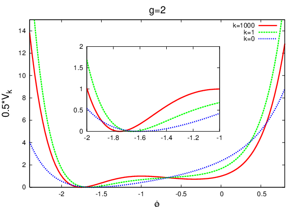
One important difference is that we have a flow equation for the superpotential and not for the effective potential itself. As a consequence, the flow equation tends to make the superpotential convex but not necessarily the effective potential. Figure 1 shows the flow of the effective potential $V_{k}$ in the polynomial approximation (38) with $N=6$ for a convex and non-convex $W_{\rm cl}$ .

Refer to caption — Figure 1: The effective potential $V_{k}$ in the *polynomial approximation* for $W_{\rm cl}^{\prime}(\phi)=1+\phi+g\phi^{2}+\phi^{3}$ . The left panel shows the potential for $g=0$ and the right panel for $g=2$ .

4.1.2 Partial differential equation

It is known from the study of non-supersymmetric systems that the polynomial approximation fails for nonconvex potentials [12, 15]. The latter require a solution of the full partial differential equation (36), which we did with NDSolve of Mathematica. In practice, we have chosen $\phi$ in the range of $\phi\in(-200,200)$ and kept the potential at its classical values on the boundary of this range. The results for three different scales are depicted in Figure 2.

For convex superpotentials, the solutions obtained from the polynomial expansions and from solving the partial differential equation are almost identical. But in the non-convex case, the polynomial expansion fails to reproduce the correct asymptotic form of the superpotential. Non-convex classical superpotentials pose a numerical challenge as they might lead to instabilities originating from the singularity at $W_{k}^{\prime\prime}(\phi)=-k$ . For such potentials – corresponding to a large coupling $g$ – the flow equation also does not reproduce the correct gap energies $E_{1}(g)$ ; see the PDE row in Table 1. We shall see that similar conclusions hold for other regulators in the flow equation.

4.2 Exponential and $\theta$ regulator

We want to compare the results obtained with the Callan-Symanzik regulator – which serves only as an IR regulator but does not suppress the UV – with an exponential and a $\theta$ regulator,

	$\displaystyle r^{(\text{e})}_{1}(p^{2},k)$	$\displaystyle=k\cdot e^{-p^{2}/k^{2}}$		$\displaystyle\text{exponential regulator}$		(39)
	$\displaystyle r^{(\theta)}_{1}(p^{2},k)$	$\displaystyle=\sqrt{k^{2}-p^{2}}\cdot\theta(k^{2}-p^{2})$		$\displaystyle\theta\text{ regulator.}$		(39)

In contrast to the infrared Callan-Symanzik regulator used in (36), these regularize the IR and UV. The corresponding flow equations for the superpotential read

	$\displaystyle\partial_{k}W^{(\text{e})}_{k}(\phi)$	$\displaystyle=\frac{1}{2k^{2}}\int\limits_{-\infty}^{\infty}\frac{dp}{2\pi}\frac{(k^{2}+2p^{2})e^{-p^{2}/k^{2}}}{p^{2}+(W^{\prime\prime}_{k}(\phi)+ke^{-p^{2}/k^{2}})^{2}}$		(40)
	$\displaystyle\partial_{k}W^{(\theta)}_{k}(\phi)$	$\displaystyle=\frac{1}{4\pi}\frac{k}{\|k^{2}-{W^{\prime\prime}_{k}}^{\,2}\|}\left(\pi\left(1-\hbox{sign}\,W^{\prime\prime}_{k}\right)+2\arctan\frac{\|k^{2}-{W^{\prime\prime}_{k}}^{2}\|}{2kW^{\prime\prime}_{k}}\right).$		(40)

Note, that for the $\theta$ regulator the integral (35) can be calculated analytically. The numerical results in Table 2 have been obtained from the solutions to these partial differential equations. For the exponential regulator we have taken $\phi\in(-20,20)$ and the integration over $p$ from $-5k$ to $5k$ . For the $\theta$ regulator, we have used $\phi\in(-50,50)$ .

g	0.0	0.2	0.4	0.6	0.8	1.0	1.2	1.4	1.6	1.8
CS	2.203	2.137	2.062	1.979	1.890	1.798	1.710	1.633	1.584	1.590
exp	2.195	2.130	2.055	1.972	1.884	1.791	1.701	1.622	1.569	1.684
$\theta$	2.197	2.132	2.058	1.975	1.888	1.794	1.705	1.626	1.576	1.581
exact	2.022	1.970	1.905	1.827	1.738	1.639	1.534	1.426	1.323	1.235

Table 2: Energy of the first excited state for the classical superpotential (37) with

(e,m,a)=(1,1,1)

and varying

g

calculated from the solution to the partial differential equation (35) with Callan-Symanzik, exponential and

\theta

regulators.

The results for the three different regulators are depicted in Table 2. They are almost identical, but all differ on the $\sim 10\%$ level from the exact values displayed in the last row of the table. Higher precision thus requires a next-to-leading order calculation in the derivative expansion including a wave-function renormalization.

5 Wave function renormalization

To next-to-leading-order in the derivative expansion, a field-dependent wave function renormalization is included in the truncation,

$\displaystyle\Gamma_{k}[\phi,F,{\bar{\psi}},\psi]$	$\displaystyle=\int d\tau d\theta d\bar{\theta}\left[\frac{1}{2}\mathcal{Z}_{k}(\Phi)K\mathcal{Z}_{k}(\Phi)+i\cdot W_{k}(\Phi)\right]$
	$\displaystyle=\int d\tau\left[\frac{1}{2}\mathcal{Z}^{\prime}_{k}(\phi)^{2}\dot{\phi}^{2}-i\mathcal{Z}^{\prime}_{k}(\phi)^{2}\bar{\psi}\dot{\psi}-i\mathcal{Z}^{\prime}_{k}(\phi)\mathcal{Z}^{\prime\prime}_{k}(\phi)\dot{\phi}\bar{\psi}\psi+\frac{1}{2}\mathcal{Z}^{\prime}_{k}(\phi)^{2}F^{2}\right.$
	$\displaystyle\left.\phantom{\int d\tau[\frac{1}{2}+}-\mathcal{Z}_{k}^{\prime\prime}\mathcal{Z}_{k}^{\prime}F\bar{\psi}\psi+iFW^{\prime}_{k}(\phi)-iW^{\prime\prime}_{k}(\phi)\bar{\psi}\psi\right]$	(41)

with a field dependent function $\mathcal{Z}_{k}(\phi)$ . The operator $K$ has been defined in (14) and primes denote derivatives with respect to $\phi$ . The results of the last sections are recovered for $\mathcal{Z}_{k}(\Phi)=\Phi$ .

In the spirit of functional optimization [8], we choose a spectrally adjusted regulator [33, 34] which includes the wave function renormalization,

\displaystyle\Delta S_{k}=\frac{1}{2}\int d\tau d\theta d\bar{\theta}\;\mathcal{Z}_{k}^{\prime}(\bar{\Phi})^{2}\Phi\left(ir_{1}+r_{2}K\right)\Phi\,,

(42)

where $\mathcal{Z}_{k}^{\prime}$ is evaluated at a background field $\bar{\Phi}=(\bar{\phi},0,0)$ . The value of $\bar{\phi}$ can be viewed as a parameter labeling a class of regulator functions. In components, the cutoff action reads

\displaystyle\Delta S_{k}=\int d\tau\;\mathcal{Z}_{k}^{\prime}(\bar{\phi})^{2}\left(\frac{1}{2}p^{2}\phi r_{2}\phi+\frac{1}{2}Fr_{2}F+iFr_{1}\phi+\bar{\psi}(pr_{2}-ir_{1})\psi\right)\,.

(43)

Again, the flow of $\mathcal{Z}_{k}$ can be read off from various operators. The simplest choice is given by the prefactor of the $F^{2}$ term, cf. eq. (41), since no time derivatives are involved here. After the projection onto the $F^{2}$ term at vanishing $\bar{\psi}\psi$ and a constant scalar field, we obtain the flow equations for the Callan-Symanzik regulator

	$\displaystyle\partial_{k}W^{\prime}_{k}(\phi)=$	$\displaystyle-W^{\prime\prime\prime}_{k}\frac{\mathcal{N}}{4{\mathcal{D}}^{2}}$		(44)
	$\displaystyle\mathcal{Z}^{\prime}_{k}(\phi)\partial_{k}\mathcal{Z}^{\prime}_{k}(\phi)=$	$\displaystyle\left(\frac{4\mathcal{Z}^{\prime\prime}_{k}(\phi)W^{\prime\prime\prime}_{k}(\phi)}{{\mathcal{D}}}-\big(\mathcal{Z}_{k}^{\prime\prime}(\phi)\mathcal{Z}^{\prime}_{k}(\phi)\big)^{\prime}-\frac{3\mathcal{Z}_{k}^{\prime}(\phi)^{2}W^{\prime\prime\prime}_{k}(\phi)^{2}}{4{\mathcal{D}}^{2}}\right)\frac{\mathcal{N}}{4\mathcal{D}^{2}}\,,$		(44)

where we have introduced the abbreviations

\displaystyle\mathcal{N}=(1+k\partial_{k})\mathcal{Z}^{\prime}_{k}(\bar{\phi})^{2}\quad\hbox{{and}}\quad\mathcal{D}=W^{\prime\prime}(\phi)+k\mathcal{Z}^{\prime}_{k}(\bar{\phi})^{2}\,.

(45)

To solve this system of coupled equations, we need to pick a value for the background field $\bar{\phi}$ . Since we are interested in the excited-state energy, a reasonable choice would be $\bar{\phi}=\phi_{\text{min}}$ . Since $\phi_{\text{min}}$ is not a priori known but a result of the flow, this would require an iterative construction of the RG trajectory. Instead we make a technically much simpler choice and identify the background field $\bar{\phi}$ with the fluctuation field $\phi$ . Since all functions in the action are parameters of the background field $\bar{\phi}$ , e.g., $\mathcal{Z}_{k}(\phi)\equiv\mathcal{Z}_{k}(\phi,\bar{\phi})$ , identifying $\bar{\phi}=\phi$ goes along with an approximation. This becomes obvious from the fact that, e.g., $\mathcal{Z}_{k}^{\prime}(\phi,\bar{\phi}=\phi)\equiv\partial_{\phi}\mathcal{Z}_{k}(\phi,\bar{\phi})|_{\bar{\phi}=\phi}\neq\partial_{\phi}\mathcal{Z}_{k}(\phi,\phi)$ . By setting $\bar{\phi}=\phi$ , we ignore this latter difference. This approximation is well known in the context of background-field flows [35, 36], and the resulting flow can be viewed as a generalized propertime flow [37, 33]. As experience demonstrates, the error made by this approximation is outweighed by the improvement arising from the better spectral adjustment of the regulator, see, e.g., [38]. Our results indeed confirm this conjecture.

Including the wave function renormalization, the on-shell effective bosonic action at next-to-leading order in the derivative expansion is

\displaystyle\Gamma_{k}[\phi,\psi=0,\bar{\psi}=0]=\int d\tau\left[\frac{1}{2}\left(\partial_{\tau}\mathcal{Z}_{k}(\phi)\right)^{2}+V_{k}(\phi)\right],\qquad V_{k}(\phi)=\frac{1}{2}\left(\frac{W^{\prime}_{k}(\phi)}{\mathcal{Z}^{\prime}_{k}(\phi)}\right)^{2}\,.

(46)

At $k=0$ , the energy gap results from the curvature of the effective potential with respect to canonically normalized fluctuations $\chi=\mathcal{Z}(\phi)$ , for which we have the standard kinetic term $\sim(\partial_{\tau}\chi)^{2}$ . Hence, the energy of the first excited state for unbroken supersymmetry is

\displaystyle E_{1}=\lim_{k\rightarrow 0}\left.\sqrt{\frac{d^{2}V_{k}(\mathcal{Z}_{k}^{-1}(\chi))}{d\chi^{2}}}\right|_{\chi_{\text{min}}=\mathcal{Z}(\phi_{\text{min}})}{=}\lim_{k\rightarrow 0}\frac{W^{\prime\prime}(\phi)}{(\mathcal{Z}^{\prime}(\phi))^{2}}\bigg|_{\phi=\phi_{\text{min}}}.

(47)

In Table 3, the energy gap $E_{1}(g)$ for $(e,m,a)=(1,1,1)$ and various couplings $g$ is compared with those obtained without wave function renormalization. The flow with wave function renormalization leads to much better results as compared to the flow without wave function renormalization. The agreement is very satisfactory with errors on the $\sim 1\%$ level even for couplings of order 1. We conclude that the flow equation is able to capture nonperturbative physics in supersymmetric quantum systems with a reasonable precision.

g	0.0	0.2	0.4	0.6	0.8	1.0	1.2	1.4	1.6	1.8
PDE	2.203	2.137	2.062	1.979	1.890	1.798	1.710	1.633	1.584	1.590
PDE+WF	2.089	2.031	1.961	1.879	1.788	1.690	1.589	1.489	1.402	1.341
exact	2.022	1.970	1.905	1.827	1.738	1.639	1.534	1.426	1.323	1.235

Table 3: Energy of the first excited state for the classical superpotential (37) with

(e,m,a)=(1,1,1)

and varying

g

calculated from the solution to flow equations with Callan-Symanzik regulator without and with wave function renormalization.

6 Summary of the numerical results

6.1 The energy of the first excited state

We find that the polynomial approximation and the solution of the partial differential equation without wave function renormalization for convex superpotentials converge to the same value independent of the regulator, see Sect. 4.1.1. Depending on the parameters of the classical superpotential, we obtain an accuracy of 10% for a small mass parameter $(m\approx 1)$ and 2% for larger mass parameters $(m\approx 3)$ . Inclusion of the wave function renormalization improves the results for the energy gap considerably. We achieve an accuracy of 3% for $m=1$ . Due to the presence of the auxiliary field, the wave function renormalization has contributions of order $p^{0}$ in the momentum and the $F^{2}$ -term – which is neglected without wave function renormalization – contributes to the on-shell potential $V_{k}(\phi)$ . This effect is more pronounced for small mass parameters as the anomalous dimension scales with the inverse of $m$ . For large $m$ , the anomalous dimension is small so we do not expect large contributions in agreement with the numerical results. Figure 3 summarizes the results for the energies $E_{1}(g)$ obtained from the different approximation schemes for $m=1$ and $m=3$ . The explicit values are listed in Tables 1-3.

The parameter space of large- $a$ couplings is explored in Fig. 4. Here, we have used $e=m=g=1$ , implying that the initial potential is always convex. First, we observe that the excited-state energy from the polynomial expansion converges rapidly to that taken from the full solution at leading-order. The deviations from the exact result are again on the $\sim 10\%$ level. This is greatly improved at next-to-leading-order including the wave function renormalization. Here, the results match the exact values with an error on the 1% level or below. The agreement holds over the whole coupling range from the weak- to the deeply nonperturbative strong-coupling regime.

The overall picture confirms that the functional RG employing the super-covariant derivative expansion captures the physics of the first excited state well beyond the perturbative small-coupling regime. For initial boundary conditions given in terms of classical convex potentials, the derivative expansion appears to converge well and reaches a very satisfactory accuracy level already at next-to-leading order.

For combinations of couplings where the initial potential is non-convex, e.g., $g>\sqrt{3}$ for $e=m=a=1$ , there is clearly room for improvements, as the deviations of the excited-state energy from the exact result become large. Though the inclusion of a wave function renormalization at next-to-leading order improves the result significantly, the accuracy remains poor, see Fig. 3. Moreover, as the next-to-leading-order correction becomes of the same order as the leading order, the convergence of the derivative expansion may become questionable. On the other hand, it is important to note in this context that the hierarchy of the derivative expansion is interwoven more strongly for the supersymmetric version than for non-supersymmetric systems. In the present case, also next-to-next-to-leading order operators can contribute to the flow of the superpotential. These contributions may be relevant for non-convex initial potentials and thus restore the convergence properties of the derivative expansion.

6.2 The global structure of the effective potential

Whereas the polynomial expansion does rather well for the excited-state energy for the convex case, we observe its break-down beyond this restricted case: For instance for $g^{2}>3$ at $e=m=a=1$ , the classical superpotential ceases to be convex. Here, the polynomial approximation fails for asymptotic values of the field, since it tries to provide for a polynomial solution of the partial differential equation near the expansion point, where the low-energy effective potential $V_{k}$ becomes flat. The global structure of the effective potential for $g=2$ calculated from the partial differential equation (36) and the polynomial approximation with Callan-Symanzik regulator are plotted in Figure 5 together with the classical potential.

As expected the polynomial approximation is not able to reproduce the correct global structure whereas the partial differential equation is able to do so. The other regulators lead to the same global structure of the effective potential.

7 Conclusions

In this paper, we have presented a functional RG approach to supersymmetric quantum mechanics. Our approach is formulated in terms of an exact and manifestly supersymmetric flow equation for the effective action which is a supersymmetric variant of the Wetterich equation. We have used the supersymmetric off-shell formulation which is the crucial ingredient to maintain the simple one-loop structure of the flow equation. The approach can straightforwardly be generalized to other supersymmetric models based on a real superfield.

We solve the flow equation nonperturbatively in a systematic and consistent approximation scheme based on an expansion of the effective action in powers of field operators of increasing numbers of supercovariant derivatives. To leading order, this yields a flow equation for the superpotential – a supersymmetric analogue of the local-potential approximation; a field dependent wave function renormalization appears in the flow to next-to-leading order.

In the present work, we focus on unbroken supersymmetry by considering only superpotentials whose highest power is even. As a physical observable, we concentrate on the energy of the first excited state resulting from the effective potential. A comparison with the exact solution provides information about the convergence of the derivative expansion. Our results confirm that the functional RG is indeed capable of describing the system over the whole range from weak to strong coupling. Our approach works particularly well for initial convex potentials. Here, first quantitative estimates can already be obtained from a simple polynomial expansion of the superpotential. For the excited-state energy, the polynomial expansion also converges nicely, whereas the solution of the full partial differential equation for the superpotential is required for global properties of the potential. Since the excited-state energy is a physical quantity, it should also be universal in an RG sense. In fact, our results show little dependence on the regulator which confirms this required universality. At next-to-leading order, the inclusion of a wave function renormalization improves the quantitative accuracy considerably. For convex potentials, the functional RG result agrees with the exact result within an error on the $\sim 1\%$ level even at strong coupling.

As soon as the initial potential becomes non-convex, the flow-equation result for the energy to lowest order starts to deviate significantly from the exact result. As is already known from standard quantum mechanics, the relevant tunneling processes are associated also with higher orders in the derivative expansion. Inclusion of the wave function renormalization indeed improves our result, even though sizable deviations from the exact result still remain. The reason for this can be anticipated: supersymmetry forces us to organize the expansion in powers of the super-covariant derivative. This, however, mixes different orders of time derivatives; e.g, in the off-shell version of any supersymmetric theory with a scalar multiplet, the auxiliary field and the derivative of the scalar field occur on equal footings. This is visible, for example, in the supersymmetry transformation of $\psi$ being proportional to $\dot{\phi}-iF$ , see (4). On the other hand, we expect that the low-lying excitation energies are mainly determined by the long-wavelength fluctuations, such that an expansion in time derivatives of the field should be well justified.

The crucial observation in this context is that the super-covariant derivative expansion contains terms without time derivatives also at higher super-covariant derivative order, for instance, $\Phi[(D\bar{D})\Phi]^{2}\sim F^{3}+\dots$ . In particular, these $F$ -potential terms can directly contribute to the flow of the superpotential. Since these terms are generated sizably only at larger values of the coupling, it is natural to expect that they can exert a pronounced influence on the energy gap at large coupling. As even higher-order operators will not take a direct influence on the flow of the superpotential, it is conceivable that the excited-state energy converges at this next-to-next-to-leading order of the super-covariant derivative expansion. Otherwise, the convergence and use of this expansion in the tunneling regime would be questionable.

A study of these higher orders giving access to operators with higher powers of $F$ are also needed for the case of broken supersymmetry. In this case, a nonzero vacuum expectation value of $F$ is expected to occur, the description of which requires knowledge of the effective potential of this auxiliary field.

The models considered here can be obtained by a dimensional reduction from the $2d$ Wess-Zumino model with $N=1$ supersymmetry. This in part is the reason that most structural results of the present work also apply to this two-dimensional field theory, for example to the form of the cutoff action and the structure of the flow equations. The super-covariant derivative-expansion techniques are straightforwardly generalizable. Work in this direction is in progress.

Acknowledgments.

Helpful discussions with C. Wozar and T. Fischbacher are gratefully acknowledged. GB acknowledges support by the Evangelisches Studienwerk and FS by the Studienstiftung des deutschen Volkes. This work has been supported by the DFG grants Wi 777/8-2 and Gi 328/5-1 (Heisenberg program).

Appendix A The flow equations in superspace

In this appendix we sketch the derivation of the flow equation for the superpotential in superspace. The equivalence of this manifestly supersymmetric derivation with the one in component form will be shown afterwards. The superspace-coordinates $(x,\theta,\bar{\theta})$ are denoted by $z$ .

The supertrace that defines the flow of the effective action translates into a superspace integral:

\displaystyle\partial_{k}\Gamma_{k}

\displaystyle=\frac{1}{2}\int\,dz\,dz^{\prime}\,\partial_{k}R_{k}(z,z^{\prime})G_{k}(z^{\prime},z)\,,\qquad G_{k}=(\Gamma^{(2)}_{k}+R_{k})^{-1}

(48)

As in the component formulation the fields are taken to be constant to calculate the Green’s function $G_{k}(z^{\prime},z)$ . In addition the expression is expanded in terms of the covariant derivatives $D$ and $\bar{D}$ . To zeroth order in the covariant derivatives one finds

i\int d\theta d\bar{\theta}\,\partial_{t}W(\Phi)=\frac{1}{2}\int\!\frac{dp}{2\pi}\,d\theta d\bar{\theta}\,d\theta^{\prime}d\bar{\theta}^{\prime}\,\left(i\partial_{t}r_{1}(p)+\partial_{t}r_{2}(p)K(p)\right)\times\\ \times\delta(\bar{\theta}^{\prime}-\bar{\theta})\delta(\theta^{\prime}-\theta)\frac{hK(p)-i{\mathcal{W}}^{\prime\prime}(\Phi)}{hp^{2}+({\mathcal{W}}^{\prime\prime}(\Phi))^{2}}\delta(\bar{\theta}^{\prime}-\bar{\theta})\delta(\theta^{\prime}-\theta)\,.

(49)

Note that in momentum space the operator $K=\frac{1}{2}(D\bar{D}-\bar{D}D)$ still contains derivatives with respect to the Grassmann-coordinates. These derivatives act on the first entry of the adjacent delta-functions. The only two contributions that remain after an integration over $\theta^{\prime}$ and $\bar{\theta}^{\prime}$ are the ones where the highest Grassmann derivative acts on one and only one of the delta functions inside the integral. Therefore we get

\displaystyle\int d\theta d\bar{\theta}\,\partial_{t}W(\Phi)=\frac{1}{2}\int\!\frac{dp}{2\pi}\,d\theta d\bar{\theta}\,\left(\frac{h\partial_{t}r_{1}(p)-{\mathcal{W}}^{\prime\prime}(\Phi)\partial_{t}r_{2}(p)}{hp^{2}+({\mathcal{W}}^{\prime\prime}(\Phi))^{2}}\right).

(50)

For the lowest component of the superfield this is exactly the flow equation (32).

To prove the equivalence of this derivation to the one in given in the main body of the paper we observe that the transition from component to superfield formulation can be achieved with the linear operators $P(\theta,\bar{\theta})=(1,\bar{\theta}\theta,-\theta,\bar{\theta})$ and $P^{T}(\theta,\bar{\theta})=(1,\bar{\theta}\theta,\theta,-\bar{\theta}):$

	$\displaystyle\Phi$	$\displaystyle=P_{i}(\theta,\bar{\theta})(\phi,F,\bar{\psi},\psi)_{i}=(1,\bar{\theta}\theta,-\theta,\bar{\theta})_{i}(\phi,F,\bar{\psi},\psi)_{i}=\phi+\bar{\theta}\psi+\bar{\psi}\theta+\bar{\theta}\theta F$
		$\displaystyle=(\phi,F,\bar{\psi},\psi)_{i}(1,\bar{\theta}\theta,\theta,-\bar{\theta})_{i}=(\phi,F,\bar{\psi},\psi)_{i}P^{T}_{i}(\theta,\bar{\theta})\,.$		(51)

In the other direction the operator $Q(\theta,\bar{\theta})=(\bar{\theta}\theta,1,-\bar{\theta},-\theta)$ must be applied:

\displaystyle(\phi,F,\bar{\psi},\psi)_{i}

\displaystyle=\int d\theta d\bar{\theta}\,Q_{i}(\theta,\bar{\theta})\Phi=\int d\theta d\bar{\theta}\,(\bar{\theta}\theta,1,-\bar{\theta},-\theta)_{i}\,(\phi+\bar{\theta}\psi+\bar{\psi}\theta+\theta\bar{\theta}F)\,.

(52)

Note that as expected $P_{i}(\theta^{\prime},\bar{\theta}^{\prime})Q_{i}(\theta,\bar{\theta})=Q_{i}(\theta^{\prime},\bar{\theta}^{\prime})P^{T}_{i}(\theta,\bar{\theta})=\delta(\bar{\theta}^{\prime}-\bar{\theta})\delta(\theta^{\prime}-\theta)$ and $\int d\theta d\bar{\theta}\,Q_{i}(\theta,\bar{\theta})P_{j}(\theta,\bar{\theta})=\int d\theta d\bar{\theta}\,P^{T}_{i}(\theta,\bar{\theta})Q_{j}(\theta,\bar{\theta})=\delta_{ij}$ . The operator $R_{k}$ and its inverse can be easily translated from component to superspace formulation using these operators:

	$\displaystyle(R_{k}(x,x^{\prime}))_{ij}$	$\displaystyle=\int d\theta d\bar{\theta}\,d\theta^{\prime}d\bar{\theta}^{\prime}\,P^{T}_{i}(\theta,\bar{\theta})R_{k}(z,z^{\prime})P_{j}(\theta^{\prime},\bar{\theta}^{\prime})$		(53)
	$\displaystyle(R_{k}(x,x^{\prime}))^{-1}_{ij}$	$\displaystyle=\int d\theta d\bar{\theta}\,d\theta^{\prime}d\bar{\theta}^{\prime}\,Q_{i}(\theta,\bar{\theta})(R_{k}(z,z^{\prime}))^{-1}Q_{j}(\theta^{\prime},\bar{\theta}^{\prime})\,,$		(54)

with $\int dz^{\prime}R_{k}(z,z^{\prime})(R_{k}(z^{\prime},z))^{-1}=\delta(z-z^{\prime})$ . So the flow equations translate into

$\displaystyle\int$	$\displaystyle dxdx^{\prime}(-1)^{\varepsilon_{i}}\partial_{t}R_{k}(x,x^{\prime})_{ij}G_{k}(x^{\prime},x)_{ji}$
	$\displaystyle=\int d\theta d\bar{\theta}\,d\theta^{\prime}d\bar{\theta}^{\prime}\,dxdz^{\prime\prime}(-1)^{\varepsilon_{i}}Q_{i}(\theta,\bar{\theta})P_{i}(\theta^{\prime},\bar{\theta}^{\prime})(\partial_{t}R_{k})(x,\theta,\bar{\theta};z^{\prime\prime})G_{k}(z^{\prime\prime};x,\theta^{\prime},\bar{\theta}^{\prime})$
	$\displaystyle=\int dzdz^{\prime\prime}(\partial_{t}R_{k})(z,z^{\prime\prime})G_{k}(z^{\prime\prime};z)$	(55)

with $(-1)^{\varepsilon_{i}}$ $-1$ if $i$ is a fermionic index and $1$ otherwise, since $(-1)^{\varepsilon_{i}}P_{i}(\theta,\bar{\theta})=P^{T}_{i}(\theta,\bar{\theta})$ .

Appendix B Initial conditions

Throughout this work, we have set the regulator component $r_{2}=0$ . With regard to the regulator structure (16), one may wonder whether this choice is compatible with a sufficient UV suppression of all modes. If not, the initial condition of the flow would not necessarily coincide with the microscopic (classical) action, but a separate UV renormalization would be necessary.

Indeed, it is easy to see that diagrams containing closed $F$ loops with a momentum-independent free propagator can give rise to UV divergencies signaling this insufficient UV suppression. On the other hand, closed $F$ loops do simply not contribute to the present truncation; this would require, e.g., the occurrence of $F$ self-interactions $\sim F^{3}$ which are generated only at higher-order in the super-covariant derivative expansion. Perturbatively, they occur at the two-loop level. We conclude that there is no danger from $F$ loops up to next-to-leading order in the derivative expansion.

Indeed, sufficient UV suppression can directly be verified. For large $k$ , the cutoff action $\Delta S_{k}$ dominates the action in the defining Euclidean path integral which is of the form [29]

\displaystyle e^{-\Gamma_{k}[\phi,F,\psi,\bar{\psi}]}=\int{\mathcal{D}}\varphi{\mathcal{D}}\mathcal{F}{\mathcal{D}}\chi{\mathcal{D}}\bar{\chi}e^{-S[\phi+\varphi,F+\mathcal{F},\psi+\chi,\bar{\psi}+\bar{\chi}]}e^{\frac{\delta\Gamma_{k}}{\delta\phi}\varphi+\frac{\delta\Gamma_{k}}{\delta F}\mathcal{F}+\frac{\delta\Gamma_{k}}{\delta\psi}\chi+\frac{\delta\Gamma_{k}}{\delta\bar{\psi}}\bar{\chi}-\varphi r_{1}\mathcal{F}-\chi r_{1}\bar{\chi}}\,.

(56)

The integral becomes dominated by small fluctuations around the classical solutions in the presence of the cutoff. A good estimate is thus provided by a saddle-point approximation of the path integral. Using the simple Callan-Symanzik regulator $r_{1}=k$ as an example, one-loop corrections are given by

\displaystyle\Gamma_{k,1\text{loop}}=-\frac{1}{2}\int\limits_{-\infty}^{\infty}\frac{dp}{2\pi}\ln\frac{S_{\phi\phi}S_{FF}-S_{F\phi}^{2}}{S_{\psi\bar{\psi}}S_{\bar{\psi}\psi}}=-\frac{1}{2}\int\limits_{-\infty}^{\infty}\frac{dp}{2\pi}\ln\left(1+\frac{iFW^{\prime\prime\prime}}{p^{2}+(W^{\prime\prime}+k)^{2}}\right).

Rescaling $p$ with $k$ yields

\displaystyle\Gamma_{k,1\text{loop}}=-k\int\limits_{-\infty}^{\infty}\frac{d\tilde{p}}{2\pi}\ln\left(1+\frac{1}{k^{2}}\frac{iFW^{\prime\prime\prime}}{\tilde{p}^{2}+(W^{\prime\prime}/k+1)^{2}}\right).

This integral vanishes for $k\to\infty$ so that no UV counterterms are necessary to define the initial conditions. The starting point of the flow equation is indeed the classical action.

References

[1] A. Feo, Predictions and recent results in SUSY on the lattice, Mod. Phys. Lett. A19 (2004) 2387–2402, [hep-lat/0410012].
[2] J. Giedt, Deconstruction and other approaches to supersymmetric lattice field theories, Int. J. Mod. Phys. A21 (2006) 3039–3094, [hep-lat/0602007].
[3] G. Bergner, T. Kaestner, S. Uhlmann, and A. Wipf, Low-dimensional supersymmetric lattice models, Annals Phys. 323 (2008) 946–988, [arXiv:0705.2212].
[4] T. Kastner, G. Bergner, S. Uhlmann, A. Wipf, and C. Wozar, Two-Dimensional Wess-Zumino Models at Intermediate Couplings, Phys. Rev. D78 (2008) 095001, [arXiv:0807.1905].
[5] K. Aoki, Introduction to the nonperturbative renormalization group and its recent applications, Int. J. Mod. Phys. B14 (2000) 1249–1326.
[6] J. Berges, N. Tetradis, and C. Wetterich, Non-perturbative renormalization flow in quantum field theory and statistical physics, Phys. Rept. 363 (2002) 223–386. hep-ph/0005122.
[7] D. F. Litim and J. M. Pawlowski, On gauge invariant Wilsonian flows, hep-th/9901063.
[8] J. M. Pawlowski, Aspects of the functional renormalisation group, Annals Phys. 322 (2007) 2831–2915, [hep-th/0512261].
[9] H. Gies, Introduction to the functional RG and applications to gauge theories, hep-ph/0611146.
[10] H. Sonoda, The Exact Renormalization Group – renormalization theory revisited –, arXiv:0710.1662.
[11] A. Horikoshi, K.-I. Aoki, M.-a. Taniguchi, and H. Terao, Non-perturbative renormalization group and quantum tunnelling, hep-th/9812050.
[12] A. S. Kapoyannis and N. Tetradis, Quantum-mechanical tunnelling and the renormalization group, Phys. Lett. A276 (2000) 225–232, [hep-th/0010180].
[13] D. Zappala, Improving the Renormalization Group approach to the quantum-mechanical double well potential, Phys. Lett. A290 (2001) 35–40, [quant-ph/0108019].
[14] M. Weyrauch, Functional renormalization group: Truncation schemes and quantum tunneling, Journal of Molecular Liquids 127 (2006) 21–27. International Conference on Physics of Liquid Matter: Modern Problems.
[15] M. Weyrauch, Functional renormalization group and quantum tunnelling, J. Phys. A39 (2006) 649–666.
[16] E. Witten, Dynamical Breaking of Supersymmetry, Nucl. Phys. B188 (1981) 513.
[17] M. Bonini, M. D’Attanasio, and G. Marchesini, Renormalization group flow for SU(2) Yang-Mills theory and gauge invariance, Nucl. Phys. B421 (1994) 429–455, [hep-th/9312114].
[18] U. Ellwanger, Flow equations and BRS invariance for Yang-Mills theories, Phys. Lett. B335 (1994) 364–370, [hep-th/9402077].
[19] P. H. Ginsparg and K. G. Wilson, A remnant of chiral symmetry on the lattice, Phys. Rev. D25 (1982) 2649.
[20] Y. Igarashi, H. So, and N. Ukita, Ginsparg-Wilson relation and lattice chiral symmetry in fermionic interacting theories, Phys. Lett. B535 (2002) 363–370, [hep-lat/0203019].
[21] G. Bergner, F. Bruckmann, and J. M. Pawlowski, Generalising the Ginsparg-Wilson relation: Lattice supersymmetry from blocking transformations, arXiv:0807.1110.
[22] F. Vian, Supersymmetric gauge theories in the exact renormalization group approach, hep-th/9811055.
[23] M. Bonini and F. Vian, Wilson renormalization group for supersymmetric gauge theories and gauge anomalies, Nucl. Phys. B532 (1998) 473–497, [hep-th/9802196].
[24] S. Falkenberg and B. Geyer, Effective average action in N = 1 super-Yang-Mills theory, Phys. Rev. D58 (1998) 085004, [hep-th/9802113].
[25] S. Arnone and K. Yoshida, Application of exact renormalization group techniques to the non-perturbative study of supersymmetric field theory, Int. J. Mod. Phys. B18 (2004) 469–478.
[26] S. Arnone, F. Guerrieri, and K. Yoshida, N = 1* model and glueball superpotential from renormalization group improved perturbation theory, JHEP 05 (2004) 031, [hep-th/0402035].
[27] O. J. Rosten, On the Renormalization of Theories of a Scalar Chiral Superfield, arXiv:0808.2150.
[28] H. Sonoda and K. Ulker, Construction of a Wilson action for the Wess-Zumino model, arXiv:0804.1072.
[29] C. Wetterich, Exact evolution equation for the effective potential, Phys. Lett. B301 (1993) 90–94.
[30] T. R. Morris, Equivalence of local potential approximations, JHEP 0507, 027 (2005), [hep-th/0503161].
[31] D. F. Litim, Optimisation of the exact renormalisation group, Phys. Lett. B486, 92 (2000) [arXiv:hep-th/0005245].
[32] D. F. Litim, Optimised renormalisation group flows, Phys. Rev. D64 (2001) 105007, [hep-th/0103195].
[33] H. Gies, Running coupling in Yang-Mills theory: A flow equation study, Phys. Rev. D66 (2002) 025006, [hep-th/0202207].
[34] J. M. Pawlowski, On Wilsonian flows in gauge theories, Int. J. Mod. Phys. A16, 2105 (2001).
[35] M. Reuter and C. Wetterich, Effective average action for gauge theories and exact evolution equations, Nucl. Phys. B417 (1994) 181–214.
[36] M. Reuter and C. Wetterich, Gluon condensation in nonperturbative flow equations, Phys. Rev. D56 (1997) 7893–7916, [hep-th/9708051].
[37] D. F. Litim and J. M. Pawlowski, Completeness and consistency of renormalisation group flows, Phys. Rev. D66 (2002) 025030, [hep-th/0202188].
[38] A. Bonanno and D. Zappala, Towards an accurate determination of the critical exponents with the renormalization group flow equations, Phys. Lett. B504 (2001) 181–187, [hep-th/0010095].