Coherent operation of coupled superconducting flux qubits

Superconducting Josephson junction qubits are one of the most promising candidates for implementing quantum computation because macroscopic coherence of superconductor is robust against noises from environment. Recent experiments for superconducting charge [1] and flux [2, 3] qubits have reported much longer coherence times. For practical quantum computing also the high performance coupled-qubit operations need to be achieved. For flux qubits an XY-type of coupling between two qubits has been achieved, where only a SWAP gate operation has been demonstrated [4]. The controlled-NOT (CNOT) gate, as the basic element of the universal gate [5], provides the simplest design for scalable quantum computing. By using an Ising-type of coupling between two flux qubits, a CNOT gate operation has been experimentally demonstrated for inductively coupled flux qubits [6] with rather weak coupling.

In this study we obtain the Hamiltonian for coupled three-Josephson-junction qubits under a microwave field in weak microwave amplitude limit, consistent with usual experimental situations. The Hamiltonian is written in terms of the magnetic dipole moment of qubit which constitutes the qubit-microwave coupling constant in experiment [7] and phenomenological Hamiltonians [8]. For a proper parameter regime for the CNOT gate operation the Hamiltonian is reduced to a block-diagonalized form. Each diagonal part of the Hamiltonian corresponds to different control qubit state. The discriminating oscillations of occupation probability of coupled qubits give rise to the CNOT gate operation. With the obtained Hamiltonian for coupled qubits we show that strongly coupled qubits can achieve the high performance CNOT gate operation. The fluctuation effects of the microwave field as well as the static magnetic field are discussed. We consider, for example, phase-coupled flux qubits to achieve a strong coupling. For practical quantum computing the phase-coupling scheme of flux qubits provides a switching function. We discuss the effects of microwave on the switching operation of phase-coupled qubits.

When only a static flux is penetrating a flux qubit, the fluxoid quantization condition for the qubit loop is given by $2\pi n+2\pi f-\phi_{1}-\phi_{2}-\phi_{3}=0$ with integer $n$. The reduced flux is denoted as $f=\Phi_{{\rm st}}/\Phi_{0}$ with the static external flux $\Phi_{{\rm st}}$ threading the qubit loop and the superconducting unit flux quantum $\Phi_{0}=h/2e$. Using the relation $\phi_{1}=2\pi(n+f)-\phi_{2}-\phi_{3}$, the energy levels of the qubit is written as $E_{s}(f)=E_{J1}[1-\cos(2\pi(n+f)-\phi_{2,s}-\phi_{3,s})]+E_{J2}(1-\cos\phi_{2,s})+E_{J3}(1-\cos\phi_{3,s}),$ where $\phi_{2(3),s}$ with $s\in\{\downarrow,\uparrow\}$ is the value of $\phi_{2(3)}$ for the state $|s\rangle$ at the local minima of $U_{{\rm eff}}$ and depends on $f$. Here $|\downarrow\rangle$ ($|\uparrow\rangle$) is the diamagnetic (paramagnetic) current state of the flux qubit.

For the Rabi oscillation of a flux qubit, a microwave field with frequency $\omega$ is applied; $f_{\omega}(t)=(\Phi_{\rm mw}/\Phi_{0})\cos\omega t,$ where $\Phi_{\rm mw}=BS$ with the microwave magnetic field $B$ and the area of the qubit loop $S$. Using the fluxoid quantization condition

the effective potential of the qubit is written as $U_{{\rm eff}}(\hat{\bm{\phi}})=E_{J1}[1-\cos(2\pi(f+f_{\omega}(t))-{\phi}_{2}-{\phi}_{3})]+E_{J2}(1-\cos{\phi}_{2})+E_{J3}(1-\cos{\phi}_{3})$ with $n=0$. Normally, in usual experiments, the applied microwave fields are in the range of $\Phi_{\rm mw}\ll\Phi_{0}$. Then, the effective potential is written as

where $\phi_{2(3),s}$ can be assumed to be constant in time due to $\Phi_{\rm mw}\ll\Phi_{0}$.

In the basis of the qubit current sates $\{\left|\uparrow\right\rangle,\left|\downarrow\right\rangle\}$ one can obtain the qubit Hamiltonian. The diagonal components $E_{\omega,s}$ of the qubit Hamiltonian consist of the static $E_{s}$ and oscillating parts; $E_{\omega,s}(t,f)\simeq E_{s}(f)-M_{s}B\cos\omega t$ with

where the qubit loop has the circulating current $I=-I_{c}\sin\phi_{1}$ with $I_{c}=2\pi E_{J1}/\Phi_{0}$ and the magnetic dipole moment of the qubit is $M_{s}$. Hence, in terms of the magnetic moment of the qubit loop and the interaction with the microwave field, the qubit Hamiltonian is rewritten as

where ${\cal H}_{0}=E_{\downarrow}\left|\downarrow\right\rangle\left\langle\downarrow\right|+E_{\uparrow}\left|\uparrow\right\rangle\left\langle\uparrow\right|-t_{q}(\left|\downarrow\right\rangle\left\langle\uparrow\right|+\left|\uparrow\right\rangle\left\langle\downarrow\right|)$ and $t_{q}$ is the tunneling amplitude between the two states in the qubit, which comes from the charging energy of the Josephson junctions [9]. The interaction between the magnetic dipole moment and the microwave field is described by

where we set $M_{\downarrow}\approx-M_{\uparrow}\equiv M$. Here note that, although the microwave field just threads the qubit loop, not applied on the qubit directly, the dipole magnetic moment of qubit and the microwave interact with each other through the fluxoid quantization condition of Eq. (1).

For two coupled flux qubits we consider that the left qubit is the control qubit. In this case the flux $f_{L}$ is adjusted far away from the degeneracy point so that the tunneling process $t_{L}$ in the left qubit is negligible, i.e., $t_{L}/|E_{\downarrow s}-E_{\uparrow s}|\approx 0$. As a consequence, the two-qubit Hamiltonian becomes block-diagonalized. Hence the problem is reduced to that of two independent qubits under a microwave irradiation,

where $E_{ss^{\prime}}(f_{L},f_{R})$ is the energy level of coupled qubits, $M_{L(R)s}$ is the magnetic dipole moment of the left (right) qubit in $|s\rangle$ state, and $-s$ denotes the opposite pseudo-spin state of $s\in\{\downarrow,\uparrow\}$. Here we set $M_{R\downarrow}\approx-M_{R\uparrow}\equiv M_{R}$ and $M_{L\downarrow}\approx-M_{L\uparrow}\equiv M_{L}$.

To clearly describe the Rabi-type oscillations, we employ rotated coordinates for the coupled-qubit states as $|00\rangle=\cos(\theta_{\downarrow}/2)|\downarrow\downarrow\rangle+\sin(\theta_{\downarrow}/2)|\downarrow\uparrow\rangle,~|01\rangle=-\sin(\theta_{\downarrow}/2)|\downarrow\downarrow\rangle+\cos(\theta_{\downarrow}/2)|\downarrow\uparrow\rangle,~|10\rangle=\cos(\theta_{\uparrow}/2)|\uparrow\downarrow\rangle+\sin(\theta_{\uparrow}/2)|\uparrow\uparrow\rangle,$ and $|11\rangle=-\sin(\theta_{\uparrow}/2)|\uparrow\downarrow\rangle+\cos(\theta_{\uparrow}/2)|\uparrow\uparrow\rangle$ with $\tan\theta_{s}=2t_{R}/|E_{s\downarrow}-E_{s\uparrow}|.$ Let us consider, for example, the case that the control qubit states is $|\downarrow\rangle$. Then we see the relations

If $2t_{R}/|E_{s\downarrow}-E_{s\uparrow}|=0$, i.e., $\sin\theta_{\downarrow}=0$, the off-diagonal terms in Eq. (7) does not appear so that the transition between the qubit states does not occur even for a resonant microwave field. Hence the tunneling $t_{R}$ between the states $|\downarrow\downarrow\rangle$ and $|\downarrow\uparrow\rangle$ plays a key role in responding to the microwave field. For the control qubit state $|\uparrow\rangle$ we also perform the transformation and obtain the two-qubit Hamiltonian,

where

with $\alpha_{0}=\sin\theta_{\downarrow},~\alpha_{1}=\sin\theta_{\uparrow},~\beta_{0}=\cos\theta_{\downarrow},$ and $\beta_{1}=\cos\theta_{\uparrow}$.

The Hamiltonian in Eq. (9) is valid in the weak microwave amplitude limit $\Phi_{\rm mw}\ll\Phi_{0}$. However, to perform a gate operation via a Rabi oscillation in experiments, $\Phi_{\rm mw}$ should satisfy a more strict condition that the Rabi frequency $\Omega$ is much smaller than the energy gap $\omega_{0}$, i.e.,

In this regime, the rotating wave approximation (RWA) can be applied and a well-behaved Rabi-type oscillation can be observed. In other words, the applied microwave field should be in the range of $\Phi_{\rm mw}=BS\ll\hbar\omega_{0}/I$. From the experimental parameters for the flux qubits in Ref. [10], this condition reads $\Phi_{\rm mw}\ll 10^{-3}\Phi_{0}$. For the Rabi frequency $\Omega/2\pi\approx$ 600 MHz which coincides with usual experimental situations, we find that the corresponding amplitude $\Phi_{\rm mw}\sim 10^{-4}\Phi_{0}$ provide a well-behaved Rabi-type oscillation in this study.

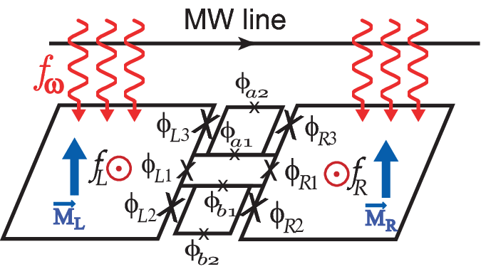
In this section, we consider a concrete system, for example, two phase-coupled qubits [11, 12, 13, 14, 15] in Fig. 1. From the Hamiltonian of Eq. (9) we show that the CNOT gate operation can be achieved with a high performance for a strong coupling. In a previous study  [11] the CNOT gate operation was analyzed without microwave irradiation. The energy levels ${\cal E}^{0}_{\rho\rho^{\prime}}(f_{L},f_{R})$ of coupled qubits are shown in Figs. 2(a) and (c) as a function of $f_{R}$ with fixed $f_{L}=0.49$.

At degeneracy points (solid lines) in Figs. 2(a) and (c), $E_{\downarrow\downarrow}=E_{\downarrow\uparrow}\equiv E_{0}$, $E_{\uparrow\downarrow}<E_{\uparrow\uparrow}$, $\theta_{\downarrow}=\pi/2$ and $\theta_{\uparrow}=\tan^{-1}(2t_{R}/|E_{\uparrow\uparrow}-E_{\uparrow\downarrow}|)$. At this point we have the diagonal elements, ${\cal E}_{00}=-t_{R}-M_{L}B\cos\omega t+E_{0}$, ${\cal E}_{01}=t_{R}-M_{L}B\cos\omega t+E_{0}$, and the constant energy gap

On the other hand, the off-diagonal term $\alpha_{0}M_{R}B\cos\omega t~(\rho=0)$ with $\alpha_{0}=1$ gives rise to a dynamical evolution between the states $|00\rangle$ and $|01\rangle$, i.e., a Rabi-type oscillation. In Figs. 2 (b) and (d) the occupation probabilities $P_{\rho\rho^{\prime}}$ of $|\rho\rho^{\prime}\rangle$ states during the Rabi-type oscillations are shown as a function of time when the initial state is prepared as $\psi(0)=(|00\rangle+|10\rangle)/\sqrt{2}$.

As shown in Fig. 2, the microwave field with the resonance frequency $\omega=\omega_{0}$ induces the Rabi oscillation between the states $|00\rangle$ and $|01\rangle$ owing to the off-diagonal term with $\rho=0$ in Eq. (9). For the weak coupling case of Fig. 2(b) the states $|10\rangle$ and $|11\rangle$ also oscillate simultaneously in response to the microwave field through the off-diagonal term $\alpha_{1}M_{R}B\cos\omega t(|10\rangle\langle 11|+|11\rangle\langle 10|)$ with $\rho=1$, while they are stationary for the strong coupling case in Fig. 2(d).

For a discriminating Rabi oscillation, the coupling strength $J$ should be larger than the tunneling rate, $J>t_{R}$. The coupling strength is given as $J=(E_{\uparrow\uparrow}-E_{\uparrow\downarrow})/4$ at the degeneracy point where $E_{\downarrow\downarrow}=E_{\downarrow\uparrow}$ [11, 12]. Further, as discussed in Eq. (11), for Rabi-type oscillations the energy gap $\omega_{0}=2t_{R}$ should be much larger than the Rabi frequency $\Omega=M_{R}B/\hbar$. Consequently, for a high performance of CNOT gate operation, we see the criteria

In Fig. 2(a), at the degeneracy point $f_{R}\approx 0.4994$, the tunneling amplitude is greater than the coupling strength, i.e., $t_{R}/h\approx 2\mathrm{GHz}$ and $J/h\approx 0.6\mathrm{GHz}$. Thus, the oscillations are not discriminative. To improve the discrimination of oscillations, one need to increase $J$ larger than the value of $t_{R}$.

From the energy levels in Fig. 2(c), increasing $J$ is shown to make the distance farther between the degeneracy point at $f_{R}\approx 0.4945$ and the other degeneracy point. This property makes it possible to perform a discriminative Rabi-type oscillation. In Fig. 2(d), we plot the oscillations of occupation probabilities $P_{\rho\rho^{\prime}}$ as a function of time by using the Hamiltonian in Eq. (9). Figure 2(d) shows that the microwave field at the resonance frequency $\omega=\omega_{0}$ induces the Rabi oscillation between the states $|00\rangle$ and $|01\rangle$ driven by the off-diagonal term for $\rho=0$ in Eq. (9), while the states $|10\rangle$ and $|11\rangle$ $(\rho=1)$ do not respond to the microwave field. From Eqs. (2) and (12) we have the relation

which shows that the difference $|\omega_{1}-\omega_{0}|$ between the energy gaps increases as the coupling strength $J$ increases at the degeneracy point. Here the the latter time-dependent term is negligibly small compared with $J$ due to the criteria of Eq. (13). Hence the states $|10\rangle$ and $|11\rangle$ hardly respond to the microwave with frequency $\omega_{0}$, resulting in the CNOT gate operation via discriminative Rabi-type oscillations at $\Omega t$=(odd)$\pi$ in Fig. 2(d).

Now we discuss the effect of fluctuations of microwave field as well as the static one on the CNOT gate operation. During the two-qubit operation both the static flux $f_{L(R)}$ and microwave flux $f_{\omega}(t)$ give rise to the noises, $\delta f_{L(R)}(t)$ and $\delta f_{\omega}(t)$, which destroy the qubit coherence. These noises appear in the fluxoid quantization condition,

Let us first discuss the noises in the left qubit. Combining the fluctuation of static flux $\delta f_{L}(t)$ into that of the microwave field $\delta f_{\omega}(t)$, the net effect of both noises is expressed as a random fluctuation $\delta B_{L}(t)$ in the microwave field $f_{\omega}(t)=(BS/\Phi_{0})\cos\omega t$. As a result, the magnetic field of microwave in the diagonal terms of Eq. (9) is rewritten as $M_{L}(B\cos\omega t+\delta B_{L}(t))$. Since the diagonal term $M_{L}(B\cos\omega t+\delta B_{L}(t))$ does not change the energy gaps $\omega_{0}$ and $\omega_{1}$ in Eqs. (12) and (14), the fluctuation $\delta B_{L}(t)$ has no effect on the operations. Hence the fluctuations of both the static and microwave fields threading the left qubit loop are negligible.

On the other hand, the fluctuations of fluxes threading the right qubit may cause the decoherence in the qubit states. Let us discuss the terms with $\rho=0$ and $\rho=1$ in Eq. (9) separately. For the $\rho=0$ terms in Eq. (9) the fluctuation of microwave flux, $\delta f_{\omega}(t)$, can be combined into the fluctuation of static flux, $\delta f_{R}(t)$, in the fluxoid quantization condition for right qubit in Eq. (15). Since the degeneracy point is optimally biased with respect to the static flux $f_{R}$, the first order fluctuation effect of both $\delta f_{R}(t)$ and $\delta f_{\omega}(t)$ on qubit state dephasing will vanish at this point.

For the terms with $\rho=1$ the net fluctuation can be given by $M_{R}(B\cos\omega t+\delta B_{R}(t))$ in the diagonal and off-diagonal terms. Since $\theta_{\uparrow}=\tan^{-1}(t_{R}/2|J|)\approx 0$ and thus $\alpha_{1}\approx 0$ for a sufficiently strong coupling, the off-diagonal term with $\rho=1$ will not appear. Thus the fluctuation $\delta B_{R}(t)$ in the off-diagonal terms hardly gives rise to dissipation of qubit states for a sufficiently strong coupling, but the fluctuations in the diagonal terms may cause dephasing.

For practical quantum computing, the quantum operations should be manipulated by a switchable coupling. To discuss this, in the model of Fig. 1, we introduce two dc-SQUIDs in the connecting loop of the phase coupled qubits. Here the external fluxes $f_{a}$ and $f_{b}$ vary from zero to 0.5. When the fluxes threading the dc-SQUID loops are set as $f_{a}=f_{b}=0$ (switch on), a dc-SQUID can be simplified as a single Josephson junction with the Josephson coupling energy $2E^{\prime}_{J}$. The design of Fig. 1 is similar to that in a previous study [12]. The difference is just the direction of pseudo-spin of the right qubit. The present design is symmetric so that it may be more appropriate for real experiments.

The current flowing in the connecting loop $I^{\prime}$ also gives rise to magnetic moments in the dc-SQUID loops. $I^{\prime}$ depends on the two-qubit states such as $I^{\prime}=\mp(2\pi/\Phi_{0})2E^{\prime}_{J}\cos\pi f^{\prime}\sin\pi f^{\prime}_{\rm eff}\equiv\pm I^{\prime}_{0}$ for the states, $|\downarrow\downarrow\rangle$ and $|\uparrow\uparrow\rangle$, respectively and otherwise $I^{\prime}=0$ [12]. Here we set $f_{a}=f_{b}=f^{\prime}.$ Then the Josephson energy of the connecting loop $U^{\prime}_{{\rm JJ},\omega}(\phi_{ai},\phi_{bi})=\sum^{2}_{i=1}[E^{\prime}_{J}(1-\cos\phi_{ai})+E^{\prime}_{J}(1-\cos\phi_{bi})]$ has an additional oscillating term,

where we used the fluxoid quantization conditions for the dc-SQUID loops and the connecting loop, $S^{\prime}$ is the area of the dc-SQUIDs, and $f^{\prime}_{\rm eff}\equiv(\phi_{L1}+\phi_{R1})/2\pi$.

As a consequence, the connecting loop energy of coupled states becomes

where $M^{\prime}_{\downarrow\downarrow}=-M^{\prime},M^{\prime}_{\uparrow\uparrow}=M^{\prime}$ and $M^{\prime}_{\downarrow\uparrow}=M^{\prime}_{\uparrow\downarrow}=0$. $M^{\prime}\equiv I^{\prime}_{0}S^{\prime}$ can be interpreted as the magnetic moment of the control loops. This magnetic moment arises by the interaction between the magnetic flux and the flowing current via the fluxoid quantization conditions of the dc-SQUID loops. If we include these terms in the Hamiltonian of Eq. (6), the net effect is just the shift of magnetic moments,

remaining the physics qualitatively the same.

The microwave field threading the dc-SQUID loops also generates noises. The noise from the microwave field can be introduced as a fluctuation of magnetic field $0.5M^{\prime}(B\cos\omega t+\delta B^{\prime}(t))$ as before. $\delta B^{\prime}(t)$ can be combined with the previous fluctuations $\delta B_{L(R)}(t)$ through the relation of Eq. (18), which does not generate qualitatively different effect. The static flux $f^{\prime}$ controls the coupling between two qubits; when $f^{\prime}=0~(0.5)$, the coupling is switched on (off). The static flux $f^{\prime}$ also generates noises in the dc-SQUID loops, but the switch-on (off) point, $f^{\prime}=0~(0.5)$, is an optimal point with respect to $f^{\prime}$ [12].

For a direct comparison of CNOT gate operation performance as the coupling strength varies, the fidelity and concurrence [16] oscillations are plotted as a function of time in Figs. 3(a) and (b). The fidelity is calculated by the definition

where $\rho_{\rm CNOT}$ is the matrix for the perfect CNOT operation and $\rho(t)$ is the truth table amplitude at time $t$ [6]. At $t=0$, $\rho(0)$ is the $4\times 4$ identity matrix and the fidelity has a finite value $F(0)=0.5$. The CNOT operation changes an initial product state into a maximally entangled state. Thus the maximal entanglement as well as the maximal fidelity corresponds to the perfect CNOT gate operation. Figure 3 shows that the deviations of the fidelity and concurrence oscillations diminish as the coupling strength increases.

At the end of two-qubit operations the phase-coupling is switched off with $f_{a}=f_{b}=0.5$. Since the magnetic dc pulse for switching-off has a finite rising time, the phase of qubit state evolves during the time, but this phase evolution is controllable by manipulating other parameters. The states of qubits can be detected by shifting the magnetic pulse adiabatically [3]. At the degeneracy point in Fig. 2, the averaged current of qubit states vanishes. Thus, one can apply a finite dc magnetic pulse to shift the qubits slightly away from the degeneracy point to detect the qubit current states.

In summary, we study the operation of two coupled flux qubits under a microwave irradiation. The flux qubits interact with the threading microwave field by the fluxoid quantization condition and can be treated as magnetic moments for a weak magnetic field threading the qubit loop. By using the coupled qubit Hamiltonian we show that for a strong coupling the microwave-driven CNOT gate can be realized with a high fidelity. The strong coupling between flux qubits is obtained by a phase-coupling scheme. Introducing the switching SQUIDs in the phase-coupled qubit results in the renomalization of the magnetic moments of both qubits. The fluctuation effects of both the static and microwave fields are discussed.

References

- [1] Wallraff A et al. 2004 Nature 431 162; Majer J et al. 2007 Nature 449 443.
- [2] Bertet P, Chiorescu I, Burkard G, Semba K, Harmans C J P M, DiVincenzo D P and Mooij J E 2005 Phys. Rev. Lett. 95 257002; Yoshihara F, Harrabi K, Niskanen A O, Nakamura Y and Tsai J S 2006 ibid. 97 167001
- [3] Kakuyanagi K, Meno T, Saito S, Nakano H, Semba K, Takayanagi H, Deppe F and Shnirman A 2007 Phys. Rev. Lett. 98 047004
- [4] Niskanen A O, Harrabi K, Yoshihara F, Nakamura Y, Lloyd S and Tsai J S 2007 Science 316 723; Niskanen A O, Nakamura Y and Tsai J S 2006 Phys. Rev. B 73 094506; Bertet P, Harmans C J P M and Mooij J E 2006 ibid. 73 064512
- [5] Barenco A et al. 1995 Phys. Rev. A 52 3457
- [6] Plantenberg J H, de Groot P C, Harmans C J P M and Mooij J E 2007 Nature 447 836
- [7] Deppe F et al. 2008 Nature Phys. 4 686
- [8] Saito S, Meno T, Ueda M, Tanaka H, Semba K and Takayanagi H 2006 Phys. Rev. Lett. 96 107001; Berns D M, Oliver W D, Valenzuela S O, Shytov A V, Berggren K K, Levitov L S and Orlando T P 2006 ibid. 97 150502
- [9] Orlando T P, Mooij J E, Tian L, van der Wal C H, Levitov L S, Lloyd S and Mazo J J 1999 Phys. Rev. B 60 15398
- [10] Mooij J E et al. 1999 Science 285 1036; van der Wal C H et al. 2000 Science 290 773; Chiorescu I et al. 2003 Science 299 1869
- [11] Kim M D and Hong J 2004 Phys. Rev. B 70 184525
- [12] Kim M D 2006 Phys. Rev. B 74 184501
- [13] Grajcar M et al. 2006 Phys. Rev. Lett. 96 047006
- [14] van der Ploeg S H W, Izmalkov A, Maassen van den Brink A, Hübner U, Grajcar M, Iĺichev E, Meyer H-G and Zagoskin A M 2007 Phys. Rev. Lett. 98 057004
- [15] Grajcar M, Liu Y-X, Nori F and Zagoskin A M 2006 Phys. Rev. B 74 172505
- [16] Wootters W K 1998 Phys. Rev. Lett. 80 2245; Hill S and Wootters W K 1997 ibid. 78 5022