On the Unicast Capacity of Stationary Multi-channel Multi-radio Wireless Networks: Separability and Multi-channel Routing

It is well known that the joint capacity of independent parallel Gaussian channels with a total power constraint is equal to the sum of the capacities of the individual channels [1]. Therefore, to find the joint capacity of the parallel channels, we can find the capacities of the individual channels separately, and then sum them up. We call such property separability in channels. The separability property may look trivial but it is not. In fact, when the noise is colored, i.e., dependent from channel to channel, the separability property in general does not hold [1].

In this paper, we first study an analogue of the above separability property for stationary multi-channel multi-radio wireless networks. Specifically, given a multi-channel multi-radio network, we define the corresponding single-channel single-radio wireless networks, and examine whether the capacity of the multi-channel multi-radio network is equal to the sum of the capacities of those corresponding single-channel single-radio networks.

We then investigate the impact of multi-channel routing on the network capacity. In a multi-channel multi-radio network, two routing schemes can be adopted: routing a given bit either (1) on multiple channels, or (2) on only one channel while different bits may be routed through different channels. We refer to the first scheme as multi-channel routing, and the second as single-channel routing. As an example, consider the routing of bit $b$ from source (node $A_{1}$), through relays (nodes $A_{2}$ and $A_{3}$), to destination (node $A_{4}$). When multi-channel routing is adopted, a route may look like:

In contrast, when single-channel routing is adopted, a route may look like:

while a different bit $b^{\prime}$ may be routed through a different channel, say, channel 3. Note that by definition multi-channel routing includes single-channel routing as a special case.

Two network models are considered: Arbitrary Network and Random Network [2]. The communication links are point-to-point with fixed data rates, and advanced techniques such as successive interference cancelation or MIMO [3] are not considered. We assume that each node has $m$ radio interfaces, and there are $c$ orthogonal channels. Due to the assumed communication model, there is no benefit for a node to simultaneously transmit (or simultaneously receive) on multiple radio interfaces on the same channel. As a result, the case $m>c$ reduces to the case $m=c$, and therefore we consider only the case $m\leq c$.

The main results are as follows:

1. 1.

   For both Arbitrary Networks and Random Networks, given a channel assignment, the separability property of network capacity does not always hold. But if $m=c$, the separability property holds.

2. 2.

   For both network models, multi-channel routing in general yields equal or a higher network capacity than single-channel routing does. But if $m=c$, the two routing schemes result in equal network capacities.

A striking difference of this paper from most existing work  [2][4][5][6][7] is that this paper deals with the network capacity and not the bounds of it. Those bounds, although very useful for studying the asymptotic or rough behavior of large wireless networks, are insufficient for studying the precise relations (i.e., being equal or unequal) to be evaluated in this paper.

The remainder of this paper is organized as follows. Section II introduces some key notations, Section III and Section IV present the results for Arbitrary Networks and Random Networks, respectively, and Section V points out some implications of the results.

A multi-channel multi-radio network $\mathcal{N}$ is a 4-tuple $(U,H,\sigma,\eta)$, where

• •

  $U:=\{1,...,n\}$ is a set of $n$ nodes, where each node $i\in U$ has $m$ radio interfaces,

• •

  $H:=\{1,...,c\}$ is a set of $c$ channels, where channel $i\in H$ supports a fixed data rate of $w_{i}$ bits/sec,

• •

  $\sigma$ is the region in which the nodes are located, and

• •

  $\eta$ is the interference model.

A channel assignment distributes the $mn$ radio interfaces onto the $c$ channels. Let $I_{i}$ be the set of radio interfaces of $\mathcal{N}$ assigned to channel $i$, $i=1,...c$. For the network $\mathcal{N}$ defined above, we define $c$ corresponding single-channel single-radio networks $\mathcal{N}_{i}^{\prime}:=(I_{i},i,\sigma,\eta)$, $i=1,...,c$. That is, $\mathcal{N}_{i}^{\prime}$ consists of the radio interfaces assigned to channel $i$, and they can communicate only on channel $i$.

A network can be configured in different ways, resulting in different data delivery capabilities. Define a network configuration $G$ as a 5-tuple $(X,I,F,M,P)$ for network $\mathcal{N}$, where

• •

  $X=(X_{1},...,X_{n})$ is the locations of the nodes, where $X_{i}$ is the location of node $i$.

• •

  $I=(I_{1},...,I_{c})$ denotes the channel assignment.

• •

  $F=(F_{1},...,F_{n})$ denotes the traffic flow configuration, where $F_{i}$ specifies a traffic flow originating from node $i$.

• •

  $M$ denotes the routing scheme, specifying the route for any source-destination pair.

• •

  $P=(P_{ij})$, $i=1,...n,j=1,2,...$ is the transmission power configuration, where $P_{ij}$ specifies the transmission power of the $j$th transmission from node $i$.

Note that when $m=c$, the optimal channel assignment $I$ is simple: a 1-1 mapping between a node’s interfaces and the channels.

In the Arbitrary Network model [2], node locations are arbitrary, each node arbitrarily chooses a destination, and the power level of each transmission is set arbitrarily. The network capacity is measured by transport capacity [2]. Following the convention in the communication theory that the term “capacity” refers to the supremum of a set of achievable “rates”, we define transport capacity as the supremum of achievable transport rates, which is defined below.

The unicast transport rate of network $\mathcal{N}$ under configuration $G$ during time interval $T$ is defined as

with unit bit-meters per second, where $l_{b}(G)$ is the distance (magnitude of the displacement) that bit $b$ travels from source to destination under configuration $G$, and $\langle T\rangle$ is the set of bits delivered within time interval $T$.

Assume that the diameter of the region $\sigma$ and the data rates $w_{i}$ are bounded. Then, transport rate $R(G,T)$ is also bounded and has a unique supremum, which we define as the unicast transport capacity

Likewise, we define the unicast transport capacity for a single-channel single-radio network $\mathcal{N}_{i}^{\prime}$ in time interval $T$

where $G_{i}^{\prime}$ configures the interfaces assigned to channel $i$ under $G$. We can also define various conditional transport capacities. For example, the network capacity conditioned on a given channel assignment $I$ is define as

where $G|I$ means that the channel assignment component of $G$ is fixed at $I$.

A few more definitions:

• •

  A tick $\tau_{i}$ is the time required to transmit 1 bit by one hop on channel $i$, i.e., $\tau_{i}=1/w_{i}$.

• •

  A Simultaneous Transmission Set (STS) of channel $i$ is a set of successful one-hop transmissions on channel $i$ in a tick.

• •

  Network $\mathcal{N}^{a}$ is said to simulate network $\mathcal{N}^{b}$, if there is a way for $\mathcal{N}^{a}$ to replicate the delivery of all the bits delivered by $\mathcal{N}^{b}$. The technique of simulation has been used in other places such as proving the equivalence of the Deterministic Finite Automaton (DFA) and the Nondeterministic Finite Automaton (NFA) [8]. We should distinguish the simulation here from what is performed by the network simulators such as the Network Simulator-2 (NS-2) [9]. With NS-2, a single computer simulates the events that occurred in a computer network, but it does not replicate real communication.

Now we present the first result Theorem III.1 below. To understand it, note that finding the transport capacity conditioned on a channel assignment involves optimization over various configuration parameters including the locations of nodes or radio interfaces. In a multi-channel multi-radio network, all interfaces of the same node must take the same location, and we call this constraint the interface location constraint. In contrast, in the corresponding single-channel single-radio networks, which are optimized independently, there is no such constraint, therefore potentially resulting in a different conditional transport capacity.

Let the optimal configuration conditioned on $I$ of network $\mathcal{N}$ be $G^{*}$. Since the nodes are distributed over 3 channels, there must be 3 or 4 simultaneous transmissions in $\mathcal{N}$ in any tick under $G^{*}$: 1 or 2 simultaneous transmissions on channel 1, and 1 transmission on channel 2 and channel 3 each.

For network $\mathcal{N}$, the optimal routing conditioned on channel assignment $I$, denoted by $M^{*}$ is such that each flow consists of only one hop. This way, the distance of each transmission is fully accounted in the transport rate while the maximum number of simultaneous transmissions can be achieved. As a result, $C(T|I)=R(G^{*},T)=\sum_{i=1}^{3}R_{i}(G^{*},T)$, where $R_{i}(G^{*},T):=\frac{1}{T}\sum_{b\in\langle T,i\rangle}l_{b}(G^{*})$ with $\langle T,i\rangle$ defined as the set of bits delivered on channel $i$ in $T$. By the definition of $C_{i}^{\prime}(T|I)$, we have $R_{i}(G^{*},T)\leq C_{i}^{\prime}(T|I)$, and hence

Now consider the optimal configurations $G_{i}^{\prime*}$ of the corresponding single-channel single-radio networks $\mathcal{N}_{i}^{\prime}$, $i=1,2,3$. It is clear that $G_{2}^{\prime*}$ is to place nodes 1 and 2 at the opposite ends of a diagonal of square $\sigma$ and let one node transmit a time, and $G_{3}^{\prime*}$ is similar. To achieve the equality in $\leq$ in (5), we must have $R_{i}(G^{*},T)=C_{i}^{\prime}(T)$ for all $i=1,2,3$, which, however, is impossible for some $\Delta$ as shown next.

Suppose that $G^{*}$ satisfies $R_{i}(G^{*},T)=C_{i}^{\prime}(T|I)$ for $i=2,3$. Under $G^{*}$, the interfaces in network $\mathcal{N}$ assigned to channels 2 and 3 must be at the corners of square $\sigma$. Because those interfaces come from all four nodes, the remaining interfaces, which are on channel 1, will also be at the corners. Choose $\Delta>0$ in the Protocol Model such that $G_{1}^{\prime*}$ allows two simultaneous transmissions on channel 1. It can be checked that placing all nodes at the corners of square $\sigma$ violates the constraints imposed by the Protocol Model and therefore cannot be optimal for $\mathcal{N}_{1}^{\prime}$. Thus $R_{1}(G^{*},T)<C_{1}^{\prime}(T|I)$. By (5), $C(T|I)<\sum_{i=1}^{3}C_{i}^{\prime}(T|I)$. $\Box$

We next show that if $m=c$, the transport capacity of any Arbitrary Network is separable in channels.

(b) We now show $C(T)\leq\sum C_{i}^{\prime}(T)$ as $T\to\infty$ by showing that any sequence of STS’s of network $\mathcal{N}$ can be simulated by networks $\mathcal{N}_{i}^{\prime}$, $i=1,...c$, essentially in the same amount of time. Partition $T$ into disjoint intervals $T_{j}$

For any configuration $G$, it is clear that $\sum_{b\in\langle T\rangle}l_{b}(G)=\sum_{j=1}^{c}\sum_{b\in\langle T_{j}\rangle}l_{b}(G)$.

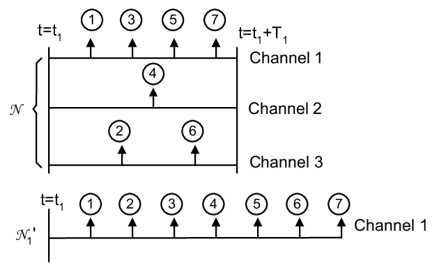
The simulation scheme is as follows: network $\mathcal{N}_{j}^{\prime}$ simulates the STS’s that occurred on network $\mathcal{N}$ during time interval $T_{j}$, $j=1,...,c$, and the $c$ simulations run simultaneously. That is, networks $\mathcal{N}_{j}^{\prime}$ each replicate a segment of the history of $\mathcal{N}$ in parallel.

There is an important dependence among the STS’s of network $\mathcal{N}$. Consider a bit that is forwarded by one hop in the current STS. This hop of forwarding contributes to the transport capacity only if the previous STS’s have completed the previous hops of forwarding. To preserve this dependence, network $\mathcal{N}_{j}^{\prime}$ schedules the STS’s in the same order they were completed in network $\mathcal{N}$ in $T_{j}$. This is illustrated in Fig. 1. In network $\mathcal{N}$ during $T_{1}$, 4 STS’s (numbered 1, 3, 5, 7) occurred on channel 1, 1 STS (numbered 4) on channel 2, and 2 STS’s (numbered 2, 6) on channel 3. The numeric order sequences the time instants at which the STS’s were completed on network $\mathcal{N}$. $\mathcal{N}_{1}^{\prime}$ simulates all 7 STS’s according to the numeric order. This way, $\mathcal{N}_{1}^{\prime}$ delivers whatever bits that were delivered by network $\mathcal{N}$ during $T_{1}$ and preserves the dependence among those bits. In general, the schedule is obtained as follows. Define $L_{ij}:=\lceil T_{j}/\tau_{i}\rceil$, the number of STS’s completed on channel $i$ during $T_{j}$. Define $\Lambda_{j}:=\{t|t=\sum_{l=1}^{j-1}T_{l}+k_{i}\tau_{i},i=1,...,c,k_{i}=1,...,L_{ij}\}$, $j=1,...,c$. That is, $\Lambda_{j}$ includes all the time instants at which the STS’s were completed on network $\mathcal{N}$ during $T_{j}$. Sorting $\Lambda_{j}$ in ascending order forms the schedule for network $\mathcal{N}_{j}^{\prime}$.

To simulate the deliveries in $\langle T_{j}\rangle$, it takes network $\mathcal{N}_{j}^{\prime}$ time

where (10) follows from (7) and that $\tau_{i}=1/w_{i}$. Also, note that $s_{j}\geq T$ because $L_{ij}=\lceil T_{j}/\tau_{i}\rceil\geq T_{j}/\tau_{i}$. We obtain the following bounds

Define $\hat{s}:=\max_{j}\{s_{j}\}$. Then $T\leq\hat{s}<T+c\max_{j}\{\tau_{j}\}$. After an elapse of $\hat{s}$, bit-meters in the amount of $\sum_{j=1}^{c}\sum_{b\in\langle T_{j}\rangle}l_{b}(G)=\sum_{b\in\langle T\rangle}l_{b}(G)$ are achieved collectively by networks $\mathcal{N}_{j}^{\prime}$, and the transport rate is

On the other hand,

where (16) follows from the definition of $C_{j}^{\prime}(T)$. Combining (16) and (13) gives

and hence, by the definition of $C(T)$,

By (a) and (b), we have $C(T)=\sum_{j}C_{j}^{\prime}(T)$, as $T\to\infty$. $\Box$

So far, we have considered $c+1$ networks: a multi-channel multi-radio network, and the $c$ corresponding single-channel single-radio networks. We next consider only one network (a multi-channel multi-radio network) but two routing schemes.

(2) This is true because with multi-channel routing, some connected links that are on different channels can be used to deliver extra bits. Consider network $\mathcal{N}$ consisting of $n=5$ nodes $A$, $B$, $C$, $D$ and $E$, $\sigma$ being a circular disk, $m=3$, and $c=9$. The channel assignment $I$, in the form of “(node: list of channels to which that node’s interfaces are assigned)”, is ($A$: 1,2,6), ($B$:3,4,7), ($C$:1,2,8), ($D$:3,5,6), ($E$:4,5,9). The data rates of the channels are $w_{i}=2,i=1,...,4$, and $w_{i}=1,i=5,...,9$. Given $I$, the optimal configuration is shown in Fig. 2 and is justified as follows. Node C must choose node A as its destination, since node A is the only node with which node C can communicate. Node A can communicate with node C on channel 1 or channel 2 and node D on channel 6. Since data rates $w_{1},w_{2}>w_{6}$, node A should choose node C as its destination. To maximize the contribution to the transport capacity, node A and node C must be at the opposite ends of a diameter, say $d_{1}$. Node D can communicate with node B on channel 3 and with node A on channel 6. Since $w_{3}>w_{6}$, node D should choose node B as its destination. To maximize the contribution to the transport capacity, node D and node B must be at the opposite ends of another diameter $d_{2}$. Now since the only remaining idle link at node B is B$\leftrightarrow$E on channel 4, node B should choose node E as its destination. To maximize the contribution to the transport capacity, node E must be at the end of diameter $d_{2}$ that is opposite node B, and thus node E is collocated with node D.

Note that under multi-channel routing, node E, node D and node A form a path E$\to$D$\to$A traversing channel 5 and channel 6. Since node E and node D are collocated, node E should choose node A as its destination. To maximum the contribution to the transport capacity, node A must be at the end of diameter $d_{2}$ that is opposite node E. Note that node A is also on diameter $d_{1}$. Thus diameter $d_{1}$ and diameter $d_{2}$ overlap. The path E$\to$D$\to$A, which makes a positive contribution to the transport capacity, is forbidden under single-channel routing. Therefore, for network $\mathcal{N}$, multi-channel routing yields a higher transport capacity, i.e., $C_{\mbox{mr}}(T|I)>C_{\mbox{sr}}(T|I)$.

(3) Now if $m=c$, we view all the interfaces on channel $j$ as a single-channel single-radio network $\mathcal{N}_{j}$. Then, by following part (b) of the proof of Theorem III.2, the STS’s under multi-channel routing can be simulated by the $c$ networks $\mathcal{N}_{j}$ in parallel. Thus, $C_{\mbox{mr}}(T)\leq\sum_{j=1}^{c}C_{j}(T)=C_{\mbox{sr}}(T)$, as $T\to\infty$, which together with $C_{\mbox{mr}}(T)\geq C_{\mbox{sr}}(T)$ completes the proof. $\Box$

In a Random Network [2], nodes are randomly located in a region. Each node randomly chooses another node as its destination, and as a result there are $n$ traffic flows in the network. The measure of network capacity is the throughput capacity [2], which is in the minimum sense since according to [2] a throughput is defined to be feasible (i.e., to be admitted in evaluating the order behavior) if all nodes can achieve it. In some scenarios, it might be beneficial to consider the average of the actual throughputs of all nodes, and this prompts us to define the average-sense (AS) throughput capacity. We call the one in [2] the minimum-sense (MS) throughput capacity. For the purpose of clarity, we give the definitions of both. But first we define the throughput of a flow originating from node $j$ during time interval $T$

with unit bits/second, where configuration $G=(X,I,F,M,P)$ is defined in Section II and $N(G,T,j)$ is the number of bits delivered by the flow originating from node $j$ in a duration of $T$. Now we define the minimum-sense (MS) throughput rate under $G$ as

where $n$ factors in the network size, and define the minimum-sense (MS) throughput capacity as

where $\mathrm{E}_{X,F}$ means taking the expected value with respect to $X$ and $F$, which are both uniform in their respective domains. We can define various conditional throughput capacities. For example, we define minimum sense (MS) throughput capacity conditioned on channel assignment $I$ as

We define the average-sense (AS) throughput rate as

As in the minimum sense case, we can also define the average-sense (AS) throughput capacity and the the average-sense (AS) throughput capacity conditioned on a channel assignment, but we leave them out for brevity. It is clear that the AS throughput capacity is not less than the MS throughput capacity. As in Section III, the corresponding single-channel single-radio networks $\mathcal{N}_{j}^{\prime}$ and their various throughput capacities can be defined as well.

We first consider the MS throughput capacity. Under channel assignment $I$, each of the corresponding single-channel single-radio networks $\mathcal{N}_{i}$ consists of two radio interfaces, and has a MS throughput capacity of $1$ bits/sec since $\sup_{0\leq x\leq 1}2\min\{x,1-x\}=1$. Therefore, $\sum_{i=1}^{c}C_{i}^{\prime}(T|I)=4$ bits/sec.

In network $\mathcal{N}$, each node can choose one of the three other nodes as its destination, resulting in $3^{4}=81$ flow configurations. Let the throughput capacity conditioned on $I$ and flow configuration $F$ be $C(T|I,F)$. It can be checked that $C(T|I,F)$ is maximized if $F$ is either $F^{\alpha}$ = (A$\to$B, B$\to$C, C$\to$D, D$\to$A) or the reverse $F^{\beta}=$(B$\to$A, C$\to$B, D$\to$C, A$\to$D), each of which results in a $C(T|I,F)$ of $4$ bits/sec. Now consider another flow configuration: $F^{\gamma}=$(A$\to$B$\to$C, B$\to$C, C$\to$D, D$\to$A), which occurs with probability $1/81$. Let the throughput of flow A$\to$B$\to$C be $x$ bits/sec, where $0\leq x\leq 1$, then the throughput of flow B$\to$C is $1-x$. The minimum of $x$ and $1-x$ is $0.5$ attained at $x=0.5$. The throughputs of the other two flows C$\to$D, D$\to$A are both $1$ bits/sec. Thus the minimum of the throughputs is $0.5$ bits/sec, and $C(T|I,F^{\gamma})=4\times 0.5=2$ bits/ec. Therefore, $C(T|I)=\mathrm{E}_{F}C(T|I,F)\leq(1/81)2+(1-1/81)4<4=\sum_{i=1}^{c}C_{i}^{\prime}(T|I)$.

We now consider the AS throughput capacity. It can be checked that $\sum_{i=1}^{c}C_{i}^{\prime}(T|I)=4$ bits/sec. Also, $C(T|I,F)$ is maximized at flow configurations $F^{\alpha}$ and $F^{\beta}$ defined above. Now consider flow configurations: $F^{\delta}$ = (A$\to$B$\to$C, B$\to$C$\to$D, C$\to$D$\to$A, D$\to$A$\to$B), each flow having two hops. Due to symmetry, each flow has a throughput of $0.5$ bits/sec, and $C(T|I,F^{\delta})=4\times 0.5=2$ bits/ec. Following the argument in the case of MS throughput capacity, we have $C(T|I)<\sum_{i=1}^{c}C_{i}^{\prime}(T|I)$. $\Box$

We next show that if $m=c$, the throughput capacity of any Random Network is separable in channels.

(2) We first prove the result for the MS throughput capacity. The result is true because the definition of MS throughput capacity may penalize single channel routing. Consider network $\mathcal{N}$ consisting of 3 nodes $A$, $B$ and $C$, $m=2$, $c=4$. The channel assignment $I$ is ($A$: 1,2), ($B$:2,3), and ($C$:3,4). There are 8 possible flow configurations, since each node can choose one of the two other nodes as its destination. Under single-channel routing, among those flow configurations, ($A\to B$, $B\to A$, $C\to B$) and ($A\to B$, $B\to C$, $C\to B$) have conditional throughput capacity $C(T|I,F)=1/2$, and the other flow configurations have a conditional throughput capacity of $0$. Thus, $C_{\mbox{sr}}(T|I)=\frac{1}{8}\frac{1}{2}+\frac{1}{8}\frac{1}{2}+0=1/8$. Under multi-channel routing, the first two flow configurations have the same conditional throughput capacity as they do under single-channel routing. Consider a third flow configuration ($A\to B$, $B\to C$, $C\to A$), which has a throughput capacity of $1/2>0$. Thus, $C_{\mbox{mr}}(T|I)>C_{\mbox{sr}}(T|I)$.

We now prove it for the AS throughput capacity. The result is true because with multi-channel routing, some connected links that are on different channels can be used to deliver extra bits. Refer to Table I for the network $\mathcal{N}$ under consideration. Network $\mathcal{N}$consists of 5 nodes $A$, $B$, $C$, $D$ and $E$, $m=2$, $c=4$, $w_{1}=1$ bits/s, $w_{2}=6$ bits/s, $w_{3}=10$ bits/s, $w_{4}=1$ bits/s. The channel assignment $I$ is ($A$: 1,2), ($B$:2,3), ($C$:3,4), ($D$:1,3), and ($E$:1,4). For flow configuration $F^{\alpha}=$($A\to C$, $C\to A$, $D\to A$, $B\to E$, $E\to D$), under single-channel routing, the throughputs are $0$, $0$, $\leq 1$, $0$, and $\leq 1$, respectively, resulting in $C_{\mbox{sr}}(T|I,F^{\alpha})\leq 2$. Under multi-channel routing, consider the following routing scheme: ($A\stackrel{{\scriptstyle 2}}{{\to}}B\stackrel{{\scriptstyle 3}}{{\to}}C$, $C\stackrel{{\scriptstyle 3}}{{\to}}B\stackrel{{\scriptstyle 2}}{{\to}}A$, $D\stackrel{{\scriptstyle 3}}{{\to}}B\stackrel{{\scriptstyle 2}}{{\to}}A$, $B\stackrel{{\scriptstyle 3}}{{\to}}C\stackrel{{\scriptstyle 4}}{{\to}}E$, $E\stackrel{{\scriptstyle 1}}{{\to}}D$). The first three flows have an aggregate throughput of $6$, and the remaining two both have $1$, resulting in an aggregate throughput of $8$ and hence $C_{\mbox{mr}}(T|I,F^{\alpha})\geq 8>C_{\mbox{sr}}(T|I,F^{\alpha})$. For any other flow configuration $F^{\beta}$, $C_{\mbox{mr}}(T|I,F^{\beta})\geq C_{\mbox{sr}}(T|I,F^{\beta})$. Taking the expected value of flow configuration completes the proof.

(3) If $m=c$, fix $X$ and $F$, and set the distance of each hop to $1$, by the proof of Theorem III.3, we have $C_{\mbox{mr}}(T|X,F)=C_{\mbox{sr}}(T|X,F)$, as $T\to\infty$. Taking the expectation of $X$ and $F$ completes the proof. $\Box$

The results of this paper apply to networks of any size, including practical networks, which have a limited number of nodes.

An implication of the separability property is that if we know the formula for calculating the capacity of single-channel single-radio networks, in general we cannot calculate the capacity of a multi-channel multi-radio network by adding up the capacities of the corresponding single-channel single-radio networks. However, if the number of interfaces at each node is equal to the number of channels, this calculation is correct.

Another implication of the separability property is that if the number of interfaces at each node is equal to the number of channels, the network capacity linearly increases with the number of interfaces at each node.

An implication of the results on multi-channel routing is that allowing a packet to be routed to a channel different from the channel on which the packet is received may improve the network capacity. However, if the number of interfaces at each node is equal to the number of channels, this routing scheme does not improve the network capacity.

This paper does not answer the question of how to achieve the network capacity. To provide the answer, a multi-commodity flow problem can be formulated [10]. However, the solution is computationally hard and only heuristic solutions have been found.

References

- [1] T. M. Cover and J. A. Thomas, Elements of Information Theory. John Wiley & Sons, Inc., 2nd ed., 2006.
- [2] P. Gupta and P. R. Kumar, “The capacity of wireless networks,” IEEE Trans. Information Theory, vol. IT-46, pp. 388–404, Mar. 2000.
- [3] D. Tse and P. Viswanath, Fundamentals of Wireless Communication. Cambridge University Press, 2005.
- [4] P. Kyasanur and N. H. Vaidya, “Capacity of multi-channel wireless networks: impact of number of channels and interfaces,” ACM MobiCom, Cologne, Germany, Aug. 2005.
- [5] L. Ma and C.-C. Shen, “Improved unicast capacity bounds for general multi-channel multi-radio wireless networks,” IEEE Communications Letters, vol. 11, pp. 874–876, Nov. 2007.
- [6] M. Franceschetti, O. Dousse, D. N. C. Tse, and P. Thiran, “Closing the gap in the capacity of the wireless networks via percolation theory,” IEEE Trans. Information Theory, vol. 53, pp. 1009–1018, Mar. 2007.
- [7] A. Keshavarz-Haddad and R. Riedi, “Bounds for the capacity of wireless multihop networks imposed by topology and demand,” ACM MobiHoc, Montreal, Quebec, Canada, Sep. 2007.
- [8] M. Sipser, Introduction to the Theory of Computation. Thomson Course Technology, 2006.
- [9] The Network Simulator - ns-2, http://www.isi.edu/nsnam/ns.
- [10] M. Kodialam and T. Nandagopal, “Characterizing the capacity region in multi-radio multi-channel wireless mesh networks,” ACM MobiCom, Cologne, Germany, Aug. 2005.