A Layered Lattice Coding Scheme for a Class of Three User Gaussian Interference Channels
Abstract
The paper studies a class of three user Gaussian interference channels. A new layered lattice coding scheme is introduced as a transmission strategy. The use of lattice codes allows for an “alignment” of the interference observed at each receiver. The layered lattice coding is shown to achieve more than one degree of freedom for a class of interference channels and also achieves rates which are better than the rates obtained using the Han-Kobayashi coding scheme.
I Introduction
Determining the capacity region of the Gaussian interference channel (IC) has been a long standing open problem. Several achievable regions and outer bounds have been obtained over the last three decades [1]–[10]. Recently, it has been shown in [7] that the Han-Kobayashi achievable region [3] achieves the capacity region of the two user Gaussian IC to within one bit. However, this result does not extend to an IC with more than two users. In [8]–[10], the sum capacity of the two user Gaussian IC has been determined for a range of “weak” interference cases.
For interference networks with more than two transmitter-receiver pairs, degrees of freedom characterization (capacity approximations within ) have been found for a class of time or frequency varying channels in [11]–[14]. These results do not apply to interference networks with channels that are not time or frequency varying. For fixed interference networks, very little is known even about its degrees of freedom characterization. In [15], some examples of user ICs are presented which come close to achieving degrees of freedom. However, for general user ICs with fixed channel gains, only one degree of freedom has been achieved, whereas the best outer bound on the total degrees of freedom is as derived in [16]. The fundamental problem, we believe, is the achievable strategy that forms the baseline of study - the Han-Kobayashi scheme [3]. In this paper, we use a layered lattice coding scheme to provide rate improvements in a three user IC over what can be obtained using the layered random coding scheme used in [3]. We also show that the layered lattice coding scheme can achieve more than one degree of freedom for a wide class of three user ICs. The results of the paper can be extended to user ICs.
The use of structured codes for ICs has already been introduced for one-sided ICs in [17] and more recently in [18] in determining capacity of very-strong ICs. Lattice coding has also been used as an effective transmission strategy in achieving the capacity of several other channels. It is used as a transmission strategy for an AWGN channel in [19]–[21] to achieve a rate close to capacity in the high SNR regime. In [22], lattice coding is shown to achieve the capacity of the AWGN channel. Some other relevant results include [23]–[29].
The rest of the paper is organized as follows: In Section II, we describe the system model for the three user Gaussian ICs and introduce the class of channels we analyze in this paper. In Section III, we introduce preliminaries on lattice coding and summarize some relevant results that we will use in this paper. In Section IV, we present the layered lattice coding approach for a symmetric three user Gaussian IC from a degree of freedom perspective. In Section V, we describe an achievable region for the symmetric three user Gaussian IC. In Section VI, we generalize the results of Sections IV to a class of non-symmetric channels. We conclude in Section VII.
II System Model
We consider the three user Gaussian IC with three transmitter-receiver pairs and three independent messages, where message originates at transmitter and is intended for receiver , for . The system model is shown in Figure and the channel equations are described by
| (1) |
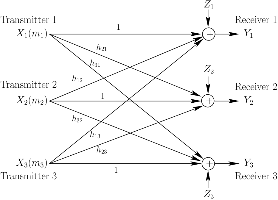
where is the received signal at the receiver at the channel use, is the transmitted signal at the transmitter at the channel use, and denotes the channel gain from the transmitter to the receiver. In the above equation, all the direct channel gains have been normalized to unity. is the zero mean, unit variance additive white Gaussian noise at receiver at time . The Gaussian noise at each receiver is i.i.d. across time. The channel inputs are subject to the following average power constraints:
| (2) |
Let denote the matrix of channel gains
Let denote a class of channel matrices such that
| (3) |
In this work, we will restrict ourselves to three-user Gaussian ICs whose channel matrices are in the set . This is the class of channels to which our coding strategy applies. Note that this is a (highly) non-trivial class of channels which includes the symmetric IC as a special case. Achievable rates and capacity region are defined in the Shannon sense. The total degrees of freedom of the three user Gaussian IC is denoted by and is defined as
| (4) |
The total degrees of freedom represents the rate of growth of sum capacity in terms of .
III Lattice Coding Preliminaries
In this section, we review some preliminaries on lattice coding and summarize some results on lattice coding that we use in this paper. A lattice of dimension is described by
where is the generator matrix that describes the lattice. Let denote the fundamental Voronoi region of the lattice and denote the volume of . In this paper, we use lattices generated using construction A described below (used in [21]).
For any positive integer , let denote the set of integers modulo . Let denote the componentwise modulo operation over integer vectors. Let denote a linear code over . Then the lattice given by
| (5) |
is generated using construction A with respect to the linear code . A set of linear codes over is “balanced” if every nonzero element of is contained in the same number of codes in . Let be the set of lattices denoted by
| (6) |
We consider a single user point to point additive noise channel
| (7) |
where is the transmitted signal, the received signal and is the additive noise of zero mean and variance equal to that corrupts the transmitted signal at the receiver. If the transmitted word over time is a lattice point, then it can be shown that a suitable lattice and a decoding strategy exists such that the probability of decoding error can be made arbitrarily small as the number of dimensions of the lattice increases. This result is stated formally in the following lemma.
Lemma 1 ([21])
Consider a single user point to point additive noise channel described in (7). Let be a balanced set of linear codes over . Averaged over all lattices from the set given in (6), each scaled by and with a fundamental volume , we have that for any , the average probability of decoding error is bounded by
| (8) |
for sufficiently large and small such that . Hence, the probability of decoding error for at least three fourths of the lattices in satisfies
| (9) |
The proof of the lemma is described in [21] and is omitted here. The next lemma describes the existence of a good lattice code for a single user AWGN channel.
Lemma 2
Consider a single user point to point additive noise channel described in (7) such that the transmitter satisfies a power constraint of . Then, we can choose a lattice generated using construction A, a shift and a shaping region such that the codebook achieves a rate with arbitrarily small probability of error if
The proof of the lemma is described in [21]. In essence, the above lemma describes the existence of a lattice code with sufficient codewords. It should be noted that lattice coding with a random dither has been used in [22] to achieve the full capacity of the AWGN channel. In the next section, we describe a layered lattice coding approach for a symmetric three user Gaussian IC from degree of freedom perspective.
IV Symmetric IC: Degrees of Freedom
In this section, we analyze the degrees of freedom of three user symmetric Gaussian IC. For this channel, the channel gain matrix is of the form
We analyze the degrees of freedom of such a channel using a layered lattice coding approach. First, we briefly review the “very strong” interference result of [18] for a symmetric three user Gaussian IC in the next lemma.
Lemma 3
[18, Theorem 2] Consider a symmetric three user Gaussian IC with channel gain , power constraint at the transmitters and noise variance at the receivers. If the channel gain satisfies , then each user can achieve a symmetric rate of .
The proof of Lemma 3 for is given in [18, Theorem 2]. The proof for any follows with little modifications. We use this lemma frequently in the next Theorem which shows that the total degrees of freedom of a symmetric three user Gaussian IC is more than for a wide range of channel parameter .
Theorem 1
Consider a symmetric three user Gaussian IC with channel parameter , and noise variance equal to . The total degrees of freedom of the channel satisfies
| (10) |
Proof:
: The proof of the Theorem for is obvious, because a simple time sharing scheme will achieve one degree of freedom for any . Hence, we focus on the other two cases.
First, we consider the case . As the channel is symmetric and we are analyzing the total degrees of freedom, we look at only symmetric rate points. For , transmitter communicates message to receiver . Transmitter splits its message into parts , such that a rate is associated with the sub-message of each message. For , the sub-message is encoded to codeword by the transmitter, which transmits . Also, each transmitter assigns a power for encoding its sub-message. Note that the subscript in rate and power does not indicate user, but the sub-messages. The power is chosen as
| (11) |
We explain the encoding and decoding strategy below in detail.
Encoding Strategy: Each transmitter encodes all its sub-messages using lattice coding, and chooses lattices , shifts and spherical shaping regions . The codebook for sub-message at each transmitters is denoted by .
Decoding Strategy: The received signal at receiver is
We denote the interference at receiver due to the sub-message from the other transmitters by given by
| (12) |
The decoding process at receiver proceeds through stages. At stage , receiver first decodes interference and then decodes message . In decoding the interference , receiver sees interference plus noise of
with an interference plus noise power . In decoding message , receiver sees an interference plus noise
with an interference plus noise power . Next, we describe the choice of lattices, shifts and spherical regions, before proceeding to probability of error analysis and rate constraints at the receivers.
Choice of Lattices, Shifts and Shaping Regions: For , each transmitter chooses shaping region to be an dimensional sphere of radius . The volume of the shaping region is denoted by . Lattice is generated using construction A such that
- •
the volume of the Voronoi region ,
- •
in decoding interference at receiver , the probability of error is upper bounded by (9) with , and
- •
in decoding message at receiver , the probability of error is upper bounded by (9) with .
Finally, shift is chosen such that the cardinality of the codebook satisfies . Next, we describe the probability of error analysis and rate constraints at receiver . The analysis and the rate constraints at other receivers are the same.
Receiver first decodes interference and message . The interference plus noise power when decoding is given by . With the choice of lattice , the probability of decoding error is upper bounded by
| (13) |
where is the volume of the Voronoi region of the lattice (the interference lattice of message and ). Hence, the probability of error decays with if
| (14) |
Similarly, in decoding the message , the interference plus noise power seen by receiver is equal to . The probability of decoding error is upper bounded by
| (15) |
Hence, the probability of error decays with if
| (16) |
Proceeding along similar lines, at stage , interference and message can be decoded successfully if
| (17) | |||
| (18) |
The power values have been chosen so that the “very strong” interference condition is satisfied at each stage. The noise plus interference power seen at stage in decoding interference and message is equal to . From the power assignments in (11), we can see that
With the choice of power values as in (11), the rate at each stage is given by
| (19) |
For to be positive, we need . Hence, the total rate achieved by each user is given by
| (20) |
Also, the total power used by each transmitter is given by
| (21) | |||||
Taking to , we get the desired result. That is,
| (22) |
Next, we consider the case . The proof for this case is very similar to that of with very few modifications. We again focus only on symmetric rates. For , transmitter splits its message into sub-parts such that rate and power is associated with the sub-message. Power is chosen as
| (23) |
The encoding strategy is similar to the one described for the case in that each transmitter uses lattice coding to encode all its sub-messages. However, the decoding strategy is slightly different. The decoding process again proceeds through stages. In stage , receiver first decodes message and then decodes interference . This is because decoding interference first will lead to rate constraints that are more binding than the constraints due to decoding the message.
Choice of Lattices, Shifts and Shaping Regions: For , each transmitter chooses shaping region to be a dimensional sphere of radius . Lattice is generated using construction A such that
- •
the volume of the Voronoi region ,
- •
in decoding interference at receiver , the probability of error is upper bounded by (9) with , and
- •
in decoding message at receiver , the probability of error is upper bounded by (9) with .
Finally, shift is chosen such that the cardinality of the codebook satisfies . The details of the probability of error analysis are similar to the case and are omitted here. Using the power assignments in (23), we see that each user achieves a rate for its sub message given by
| (24) |
Hence, each user achieves a total rate given by
| (25) |
The total power expended by each transmitter is given by
| (26) | |||||
Taking to , we get the desired result. This completes the proof of Theorem 1. ∎In Figure 2, we plot the degrees of freedom that we achieve for a symmetric three user Gaussian IC using the layered lattice coding approach.

Remark 1
From (10), we can see that the achievable total degrees of freedom tends to as the channel gain , and when . We should also see that when the channel gain , then we can achieve degrees of freedom.
V Comparing Lattice Coding and Han Kobayashi Coding
In this section, we compare our layer lattice coding approach with the extension of Han-Kobayashi scheme for the three user symmetric Gaussian IC. In the Han-Kobayashi coding scheme for the two user IC [3], each transmitter splits its message into two parts, a private part and a common part. For decoding, each receiver decodes its message and the common message transmitted by the interfering transmitter. In the extension of this scheme to the three user IC, each transmitter splits its message into four parts - one private part and three common parts. For instance, transmitter splits its message into four parts - 1) , the private part, 2) , the common part which is also decoded by receiver , 3) , the common part which is also decoded by receiver and 4) , the common part which is decoded by receivers and . We restrict ourselves to Gaussian codebooks when considering the Han-Kobayashi coding strategy. Finally, as the channel is symmetric, we compare the maximum symmetric rate that can be achieved using the two approaches. In the next Lemma, we derive a symmetric rate point that can be achieved using the layered lattice coding approach for the three user symmetric Gaussian IC with cross channel gain and power constraint . We define as follows
| (27) |
Let denote the maximum symmetric rate that can be obtained by Han-Kobayashi coding scheme in a three user symmetric Gaussian IC with power constraint , noise at the receiver and the cross channel gain equal to .
Lemma 4
Consider a symmetric three user Gaussian IC with cross channel gain and power constraint at each transmitter. Then
a) if and , each user can achieve a symmetric rate given by
| (28) |
b) If , and there exists integer such that
then each user can achieve a symmetric rate given by
| (29) |
c) If , and there exists integer such that , then each user can achieve a symmetric rate given by
| (30) |
d) If and , each user can achieve a symmetric rate of
| (31) |
e) If and there exists integer such that
then each user can achieve a symmetric rate of
f) If and there exists integer such that , then each user can achieve a symmetric rate given by
| (35) |
The proof of the above Lemma is very similar to the proof of Theorem 1 and is omitted here. It should be noted that for cases (b) and (e) in the lemma, we use Han-Kobayashi style encoding and decoding for the first layer of the codebook. This is because, the power allocated to this level is not sufficient enough to reap the advantages of lattice coding. Figure 3 compares the symmetric rate point achievable using the layered lattice coding approach with the maximum symmetric rate that can be achieved using Han-Kobayashi scheme for and . Note that in our layered lattice coding approach, we restrict ourselves to identical power splitting approach by all the transmitters. This can be generalized to different power splitting schemes and can possibly give better results. However, it is interesting to note that even a possibly suboptimal lattice coding scheme significantly outperforms the extension of the Han-Kobayashi scheme.

This shows that while the Han-Kobayashi coding scheme (message splitting and random coding) is optimal to within one bit for a two user Gaussian IC [7], it is not optimal even in terms of degrees of freedom for larger ICs with more than two transmitter-receiver pairs. The results of the paper in fact suggest that the optimal strategy might in fact be interference alignment through lattice coding. Lattice coding while allowing the interference to be decoded without decoding the interfering messages places fewer constraints on the rates of the interfering users. In particular, it eliminates the MAC type constraints that arise when decoding the interfering messages separately.
VI Generalizations to non-symmetric channels
In this section, we generalize the results of Section IV to a class of non-symmetric three user Gaussian ICs. We consider channel whose channel matrix . As , there exists integers and such that and
| (36) |
In the next Lemma, we provide a generalization of the “very strong” interference result in [18] to non-symmetric channels.
Lemma 5
Consider a three user Gaussian IC, whose channel matrix and whose channel gains satisfy (36). The power constraints at the transmitters are and the noise variances at the receivers are and . If the channel gains satisfy one of the following three equations
| (37) | |||
(or)
| (38) | |||
(or)
| (39) | |||
then, the users can achieve rates given by
| (40) |
That is, each user can achieve rates within half a bit of their maximum possible rates.
The proof of the lemma is very similar to the proof of [18, Theorem 2]. We describe below a brief outline of the proof.when the channel gains satisfy (37).
Outline of the Proof: The encoding and decoding scheme are similar to those used in [18, Theorem 2]. Each transmitter uses lattice codes to transmit their messages. For , transmitter chooses lattice generated using construction A described in (5) or in [21]. To ensure that the interference lattices are aligned at each receiver, we choose the lattices so that
| (41) |
Let denote the volume of the Voronoi region of lattice . The shaping region chosen by user is a dimensional sphere of radius denoted by . We denote the volume of by . Then, we choose the following relationship between and
| (42) |
The shifts for transmitter denoted by is chosen such that the codebook given by has at least codewords. For decoding, receiver first decodes the total interference it sees and then decodes its own message. We describe the rate constraints involved in successful decoding at receiver .
The total interference seen by receiver is given by
| (43) |
Hence, the interference signal is an element of lattice . In decoding the total interference, receiver sees a noise of whose power . Therefore, the interference can be successfully decoded if
| (44) | |||
| (45) |
After decoding the interference, receiver decodes its message. The probability of decoding error decays with if
| (46) |
The analysis for receivers and are similar to that of receiver and the details are omitted here. If the channel gains satisfy (37), then the rate constraints due to decoding interference are less binding than the rate constraints due to decoding the message at each receiver. Hence, the users can achieve rates given by
This completes the outline of the proof when the channel gains satisfy (37). Next, we analyze the degrees of freedom of non-symmetric ICs.
VI-A Degree of Freedom Analysis
In this section, we briefly analyze the degrees of freedom of three user non-symmetric Gaussian ICs. We use the same layered lattice coding scheme that we used for the symmetric case. To present the main ideas, we consider an example three user Gaussian IC with channel matrix given by
| (47) |
where . Without loss of generality we assume . The analysis for other channel matrices in are similar to the one presented and is omitted here. We describe the encoding and decoding strategy below:
For , transmitter communicates message to receiver . Transmitter splits its message into parts - such that rate is associated with the sub-message. For , transmitter encodes message into codeword and transmits . Also, transmitter assigns power to encode its sub-message.
Encoding Strategy: Each transmitter encodes all its sub-messages using lattice coding, and chooses lattices . Transmitter chooses shifts and spherical shaping regions . The codebook for the sub-message at transmitter is denoted by and is given by .
Decoding Strategy: The received signal at receiver is given by
We denote the interference at receiver due to the sub-message from the other transmitter by and is given by
The decoding process at receiver proceeds through stages. At stage , receiver first decodes interference and then decodes its sub-message . In decoding interference , receiver sees an effective noise power of
| (48) |
In decoding message , receiver sees an interference plus noise power of
| (49) |
The choice of lattices , shifts and shaping regions are similar to those described in Theorem 1 and the details are omitted here. We choose the powers such that the “very strong” interference condition is satisfied at every decoding stage. That is, at stage , the rate constraints on due to decoding interference at receiver is less binding than the constraint imposed due to decoding message at receiver . Hence, we choose powers such that
The rate achieved by user at stage is given by
| (54) |
The total power used by transmitter is given by
The total degrees of freedom then satisfies
However, unlike the symmetric channel case in Theorem 1, we have not been able to derive closed form expressions for the total degrees of freedom achievable for non-symmetric channels. We illustrate the total degrees of freedom achieved for an example channel (derived numerically) in Figure 4.

The degree of freedom analysis for other non symmetric three user Gaussian ICs with channel matrix follows along the same lines as the analysis for the channel given by (47).
VII Conclusions
In this paper, we proposed a layered lattice coding scheme for the three user Gaussian IC. In Theorem , we showed that the layered lattice coding approach can achieve more than degree of freedom for symmetric channels. We also derived an analytical expression for the achievable degrees of freedom in terms of the channel gain . In Section V, we compared the Han-Kobayashi coding strategy with our layered lattice coding scheme for symmetric ICs. We showed that significant rate benefits can be achieved by decoding the interference rather than decoding the interfering messages. Finally, in Section VI, we extended the “very strong ” interference result of [18] to a class of non-symmetric channels and used this to generalize the layered lattice coding approach to that class of channels.
References
- [1] A. Carleial, “Interference channels,” IEEE Trans. Inform. Theory, vol. 24, no. 1, pp. 60–70, Jan. 1978.
- [2] R. Benzel, “The capacity region of a class of discrete additive degraded interference channels,” IEEE Trans. Inform. Theory, vol. 25, no. 2, pp. 228–231, March 1979.
- [3] T. S. Han and K. Kobayashi, “A new achievable rate region for the interference channel,” IEEE Trans. Inform. Theory, vol. 27, no. 1, pp. 49–60, Jan. 1981.
- [4] H. Sato, “The capacity of the Gaussian interference channel under strong interference,” IEEE Trans. Inform. Theory, vol. 27, no. 6, pp. 786–788, Nov. 1981.
- [5] A. A. E. Gamal and M. H. M. Costa, “The capacity region of a class of deterministic interference channels,” IEEE Trans. Inform. Theory, vol. 28, no. 2, pp. 343–346, March 1982.
- [6] M. Costa, “On the Gaussian interference channel,” IEEE Trans. Inform. Theory, vol. 31, no. 5, pp. 607–615, Sep 1985.
- [7] R. H. Etkin, D. N. C. Tse, and H. Wang, “Gaussian interference channel capacity to within one bit,” submitted to IEEE Trans. Inform. Theory, Feb. 2007, preprint available at http://www.eecs.berkeley.edu/ dtse/interference.pdf.
- [8] X. Shang, G. Kramer, and B. Chen, “A new outer bound and the noisy-interference sum-rate capacity for Gaussian interference channels,” submitted to IEEE Trans. Inform. Theory, Dec. 2007, arXiv:0712.1987v2, e-print.
- [9] V. S. Annapureddy and V. Veeravalli, “Gaussian interference networks: sum capacity in the low interference regime and new outer bounds on the capacity region,” submitted to IEEE Trans. Inform. Theory, Feb. 2008, arXiv:0802.3495, e-print.
- [10] A. S. Motahari and A. K. Khandani, “Capacity bounds for the Gaussian interference channel,” submitted to IEEE Trans. Inform. Theory, Jan. 2008, arXiv:0801.1306, e-print.
- [11] V. R. Cadambe and S. A. Jafar, “Interference alignment and the degrees of freedom for the K user interference channel,” IEEE Trans. Inform. Theory, vol. 54, no. 8, pp. 3425–3441, Aug. 2008.
- [12] ——, “Degrees of freedom for wireless x networks,” Nov. 2007, arXiv: 0711.2824, e-print.
- [13] ——, “Capacity of wireless networks within o(log(snr)) - the impact of relays, feedback, cooperation and full-duplex operation,” Feb. 2008, arXiv: 0802.0534, e-print.
- [14] M. Shen, A. Host-Madsen, and J. Vidal, “An improved interference alignment scheme for frequency selective channels,” in Proc. of ISIT, July 2008.
- [15] V. R. Cadambe, S. A. Jafar, and S. Shamai, “Interference alignment on the deterministic channel and application to fully connected AWGN interference networks,” arXiv: 0711.2547, e-print.
- [16] A. Host-Madsen and A. Nosratinia, “The multiplexing gain of wireless networks,” in Proc. of ISIT, 2005.
- [17] G. Bresler, A. Parekh, and D. N. C. Tse, “The approximate capacity of the many-to-one and one-to-many Gaussian interference channels,” in Proc. of 45th Allerton Conference, Sept. 2007.
- [18] S. Sridharan, A. Jafrian, S. Vishwanath, and S. A. Jafar, “Capacity of symmetric -user Gaussian very strong interference channels,” to appear in Globecom Communications Conference, New Orleans, Dec. 2008, arXiv:0808.2314v1, e-print.
- [19] R. de Buda, “The upper error bound of a new near-optimal code,” IEEE Trans. Inform. Theory, vol. 21, no. 4, pp. 441–445, July 1975.
- [20] G. Poltyrev, “On coding without restrictions for the AWGN channel,” IEEE Trans. Inform. Theory, vol. 40, no. 2, pp. 409–417, March 1994.
- [21] H. A. Loeliger, “Averaging bounds for lattices and linear codes,” IEEE Trans. Inform. theory, vol. 43, no. 6, pp. 1767–1773, Nov. 1997.
- [22] U. Erez and R. Zamir, “Achieving 1/2 log(1 + SNR) on the AWGN channel with lattice encoding and decoding,” IEEE Trans. Inform. Theory, vol. 50, no. 10, pp. 2293–2314, Oct. 2004.
- [23] U. Erez, S. Litsyn, and R. Zamir, “Lattices which are good for (almost)everything,” IEEE Trans. Inform Theory, vol. 51, no. 10, pp. 3401–3416, Oct. 2005.
- [24] R. Zamir, S. Shamai, and U. Erez, “Nested linear/lattice codes for structured multiterminal binning,” IEEE Trans. Inform. Theory, vol. 48, no. 6, pp. 1250–1276, June 2002.
- [25] U. Erez, S. Shamai, and R. Zamir, “Capacity and lattice strategies for canceling known interference,” IEEE Trans. Inform. Theory, vol. 51, no. 11, pp. 3820–3822, Nov. 2005.
- [26] Y. H. Nam and H. E. Gamal, “Joint lattice decoding achieves the optimal diversity multiplexing tradeoff for multiple access channels,” submitted to IEEE Trans. Inform. Theory, April 2007.
- [27] D. Krithivasan and S. S. Pradhan, “Lattices for distributed source coding: Jointly Gaussian sources and reconstructions of a linear function,” submitted to IEEE Trans. Inform. Theory, July 2007, arXiv:0707.3461, e-print.
- [28] B. Nazer and M. Gastpar, “Lattice coding increases multicast rates for Gaussian multiple-access channels,” in Proc. of 45th Allerton Conference, Sept. 2007.
- [29] ——, “The case for structured random codes in network capacity theorems,” European Trans. on Comm, Special Issue on New Directions in Inform. Theory, vol. 19, no. 4, pp. 455–474, June 2008.