A Deep 150 MHz GMRT Survey in Eridanus
Abstract
We present results of a 150 MHz survey of a field centered on Eridani, undertaken with the Giant Metrewave Radio Telescope (GMRT). The survey covers an area with a diameter of , has a spatial resolution of and a noise level of mJy at the pointing centre. These observations provide a deeper and higher resolution view of the 150 MHz radio sky than the 7C survey (although the 7C survey covers a much larger area).
A total of 113 sources were detected, most are point-like, but 20 are extended. We present an analysis of these sources, in conjunction with the NVSS (at 1.4 GHz) and VLSS (at 74 MHz). This process allowed us to identify 5 Ultra Steep Spectrum (USS) radio sources that are candidate high redshift radio galaxies (HzRGs). In addition, we have derived the distribution for these observations and compare our results with other low frequency radio surveys.
Keywords:
surveys - galaxies: active - galaxies: starburst - radio continuum: general1 Introduction
Over the past 50 years many large radio surveys have taken place, allowing us to build up an understanding of the evolution of the radio source population (see for example, Rowan-Robinson et al. 1993). Various deep surveys have taken place, but many have been at frequencies of 1.4 GHz and higher (for obvious angular resolution reasons) and have reached down to Jy levels (e.g. Hopkins et al. 1998; Huynh et al. 2005). Probably, the most important result from these surveys is the confirmation of the upturn in the Euclidean-normalised differential source counts below mJy (Windhorst et. al. 1985) which is believed to be due to a population of sources that are not AGN (Condon 1989). The “normal” population of radio sources (with flux densities larger than a few mJy) can be explained by radio loud AGN which are hosted in elliptical galaxies. Towards Jy flux levels the radio sources counts are increasingly dominated by other populations, such as radio-quiet AGN, starbursts and late-type galaxies (with their radio emission due to massive star formation and associated supernovae).
At lower radio frequencies (below 1.4 GHz) the population of radio sources is less explored, mostly due to the relatively bright flux limits achieved at these frequencies. The Westerbork Synthesis Radio Telescope (WSRT) has been used for this purpose reaching a detection limit of mJy at 610 MHz, however this is not sufficiently deep to probe the upturn in source counts (Valentijn 1980). The Giant Metrewave Radio Telescope (GMRT) located near Pune, India, however, has the necessary capabilities (low frequency with good sensitivity) and there have been a few deep surveys using the GMRT at 610 MHz. Examples include Moss et al. (2007), Garn et al. (2007), Bondi et al. (2007) and Garn et al. (2008).
The 150 MHz sky is still less explored. Although the GMRT is capable of observations at this frequency, there have been relatively few results presented in the literature. At 150 MHz the GMRT has a spatial resolution approaching and a theoretical rms noise of around mJy. This compares favourably with the Cambridge 7C survey (Hales et al. 2007), which had a resolution of arcsec2, and a typical rms noise of around mJy. Of course, the 7C survey covers a much larger area than is covered in this survey, and the final 7C catalogue contains 43683 sources over an area of 1.7 steradians. The 7C survey region does not overlap with the field presented here.
A comparison of the point source sensitivities for a range of low frequency surveys is illustrated in Fig. 1. The point labelled “GMRT” is the survey presented here. Other surveys included the various Cambridge surveys (6C, 7C, 8C) at 38 MHz (Rees 1990) and 151 MHz (Hales et al. 2007), the XMM-LSS survey at 74 MHz and 325 MHz (Cohen et al. 2003), The VLA Low-frequency Sky Survey (VLSS) at 74 MHz (Cohen et al. 2007), The Westerbork Northern Sky Survey (WENSS) at 325 MHz (Rengelink et al. 1997), Molonglo Reference Catalogue (MRC) at 408 MHz (Large et al. 1981), the Sydney University Molonglo Sky Survey (SUMSS) at 843 MHz (Mauch et al. 2003) and the NVSS and FIRST both at 1.4GHz (Condon et al. 1998, White et al. 1997). We also show examples of what can be achieved in deeper smaller area surveys; the “GMRT 610 MHz” refer to surveys such as Garn et al. (2007) and Moss et al. (2007), which can achieve point source detections down to around 0.3 mJy, and “Deep 1.4 GHz” refers to surveys such as Huynh et al. (2005), with point source detections down to mJy.
We also show lines corresponding to sources with spectral indices of and , for a flux (which we shall adopt throughout this paper). We can see from Fig. 1 that the point source sensitivity of this GMRT survey is well matched to the NVSS. By comparing the sources detected at 150 MHz with other surveys (such as the NVSS at 1.4 GHz or the VLSS at 74 MHz) it is possible to identify sources with extreme spectral indices, which are termed Ultra-Steep Spectrum (USS) sources. In turn, these USS sources are candidates for being high-redshift radio galaxies (HzRGs).
Radio sources can be detected out to high redshift (). Empirically, it appears that the majority of high redshift radio sources tend to exhibit steeper radio spectra (see for example, De Breuck et al. 2000; Miley & De Breuck 2008). The origin for this correlation is unclear. Part of it may be due to a Malmquist bias, but it now seems likely that the higher gas densities in the galaxy environments at high redshift (constricting the development of radio bubbles from such AGN) plays a role (see Miley & De Breuck 2008 for a discussion of this). Having identified candidate HzRGs via their radio spectrum it is then necessary to identify the galaxies in the optical/IR and subsequent determine the redshift. HzRGs seem to have a relatively small scatter in a plot of -band magnitude versus , and they seem to be among the most luminous galaxies at high redshift (De Breuck et al. 2002). Apart from HzRGs there are a number of other sources that exhibit steep spectral indices. These include, but are not limited to, fossil radio galaxies, cluster halos or pulsars (Parma et al. 2007, Manchester et al. 2005).
The primary science driver behind these observations was to detect the magnetospheric radio emission from the exoplanet orbiting Eridani. No detection was made, however, tight constraints on the possible radio emission were determined and these results are summarised in George & Stevens (2007). The wide field, good sensitivity and reasonable spatial resolution of the GMRT 150 MHz observations does give an excellent view of the radio sky. From these observations, we show that deep imaging with the GMRT at 150 MHz enables us to identify candidate high redshift radio sources. Some relevant GMRT results at 150 MHz have been published by Ishwara-Chandra & Marathe (2007), although it is clear that this is still an under-exploited capability.
The observations and data analysis are described in Section 2. We discuss the generation of the catalogue in Section 3 and present an analysis of the radio source counts at 150 MHz in Section 4. We then investigate the nature of the sources, including spectral indices and identify the candidate high redshift objects in Section 5. We conclude in Section 6.

2 The GMRT 150 MHz Observations and Data Analysis
2.1 Observations
The radio observations discussed here were conducted with the GMRT, during cycle 11 on 10 August 2006 and lasted for a duration of 4.13h. The pointing centre was Eridani (RA: Dec: ). The central frequency of the observation was 157.0 MHz and a bandwidth of 8 MHz was used (split into 128 channels). For flux density calibration 3C48 was observed and for phase calibration purposes 0114–211 was used. The time on source in a single scan was 30 minutes before moving to the phase calibrator for 5 minutes. All reduction was performed with the Astronomical Image Processing System (AIPS). The visibilities from each baseline and channel were carefully inspected and edited to remove interference, cross-talk between antennas, instrumental glitches and the poor-quality data recorded at the beginning of each pointing was removed. The flux density scale was set by an AIPS implementation of the Baars et al. (1977) scale.
2.2 Imaging Strategy and Calibration

Wide-field mapping with a diameter (close to the full width of the beam) was performed over 121 facets, with the phase of the data shifted to the tangent point at the centre of each facet. This ensures that no point on any image is far from the tangential pointing position, thus we minimise the smearing of sources far from the phase tracking centre (due to the breaking of the coplanar array assumption by using a two-dimensional FFT to approximate the celestial sphere). Imaging and deconvolution was performed using the AIPS task IMAGR. The final 121 image facets used for analysis were total intensity maps, with a final restoring beam (the resolution) of . The central rms () noise level achieved was 3.12 mJy, though areas of higher rms noise surround the sources (with a typical noise of around 5 mJy, rising for the very brightest sources) and near the edges of the field. For a given flux level, we found a large number of spurious sources in the outer regions and have focused in on the central regions of the observation.
This noise level can be compared with the theoretical thermal noise limit for the GMRT at 150 MHz, given by
| (1) |
where is the telescope system temperature (615K), is the antenna gain (0.33 K Jy-1), is the number of working antennas (typically 27 during our observation), is the number of sidebands, is total time on source and MHz is the effective bandwidth for each sideband after channel collapsing11 1 . The theoretical noise limit of the GMRT is then mJy/beam. Our observations are a moderate factor above the theoretical limit. The reason for the limitation is probably due to radio frequency interference during the observations (particularly low level RFI), though limitations from the dynamic range also make a contribution. The maps of the individual facets were combined into a final mosaic using the AIPS task FLATN, with no correction made for the degradation of the primary beam sensitivity at this stage (any flux density corrections are considered later).
The final image is shown in Fig. 2. We will discuss the source detection criteria in the following section.
As we are dealing with low-frequency observations, atmospheric refraction is likely to be an issue. In order to test the positional accuracy of our sources we compared the positions of the 20 brightest objects with their 1.4 GHz counterparts in the NVSS. On average there was an offset of between our extracted source positions and the location of sources in the NVSS. We attribute this offset to refraction in the Earth’s ionosphere. This corresponds to an offset of in RA and in Dec and the listed positions in the source catalogue (Table 1) are corrected for this offset.
3 Generating the Source Catalogue

3.1 Source Extraction
The next stage is to construct a source catalogue for these observations. Because this observation was a single pointing, rather than a well constructed survey involving a series of pointings to obtain a fairly uniform sensitivity over a wide area, we have chosen to consider only the central region of the observation.
Sources were only included within a 1.07∘ radius from the pointing centre (out to the point that the primary beam correction dropped to 20 per cent of its central value) and allows us to avoid higher noise outer regions of the dataset. A rms noise map of the survey area was constructed for use within the source detection procedure. Sources are extracted using the AIPS task SAD. SAD attempts to find all sources in an image whose peak brightness is greater than a given level and then by fitting Gaussian models to the image by least squares method. During the detection process the rms is found by simply looking up the coordinate of the component in the rms noise map. In this region a conservative peak brightness detection limit of 6 (corresponding to a flux limit of 18.6 mJy) was used to minimise the number of noise spikes spuriously detected as sources. In the regions around the brightest sources the detection was performed separately using higher thresholds and visual inspection.
Within this region a total of 113 sources were found above the 6 threshold. Any extended sources for which the Gaussian model used by SAD inadequately described the data (i.e. sources with angular sizes greater than or showing some form of substructure upon visual inspection), were inspected using the AIPS task TVSTAT. There were 9 sources that this procedure was used for, at least 2 of these sources appear to be clear double-lobed sources. In Fig. 3 we present a small selection of these extended sources.
3.2 Resolution Effects
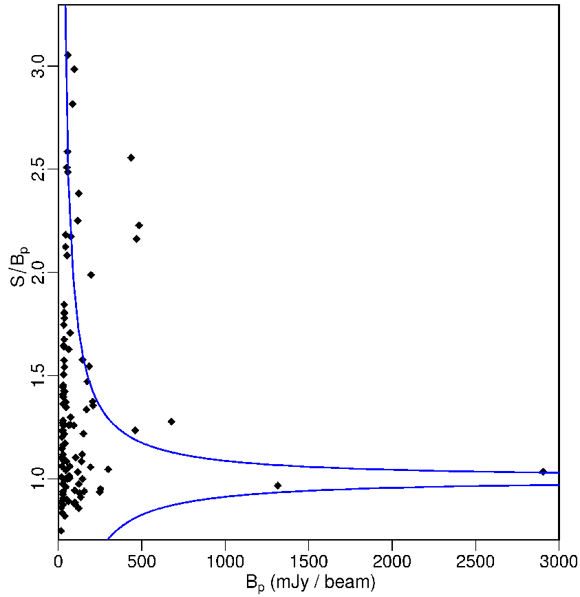
When analysing low signal-to-noise ratio detections, noise spikes can easily cause Gaussian fitting routines (such as SAD) to poorly fit the width of a source, giving inaccurate measures of the flux density. To investigate this effect, we plot the ratio between the flux density, , and the peak brightness, , as a function of the peak brightness for all the radio sources in the catalogue. Under the assumption that the measurement of any source that has a flux density less than the peak brightness is due to the effect of noise, we use the distribution of the ratio to define a criterion for a source to be considered resolved. This distribution is then mirrored above the value and can be seen in Fig. 4. Any source within this envelope is considered as unresolved and its peak brightness is taken as the best measure of its true flux density. The lower envelope contains 98 of the sources with . The upper envelope is characterised by the equation
| (2) |
Using the above envelope a total of 20 sources (18) are considered to be adequately resolved and we take their flux density as a measure of their true flux.
3.3 Flux Density Corrections
We must first consider the effect of bandwidth smearing on our data. This is seen as a radial blurring of the source. The flux density of a source is conserved but the peak brightness is reduced and this effect is the result of many channels of finite bandwidth being used in the interferometric inversion, that assumes monochromatic radiation. To minimise this effect we chose to avoid channel collapsing over a large number of channels. The total bandwidth over all the channels was 8 MHz and so, to avoid this effect, we collapsed our 128 channels (each of 62.5 kHz) to 11 channels (each of 687 kHz). This allows us to improve the noise while avoiding the effect of bandwidth smearing.
Another important effect is time-delay smearing, due to the rotation of source in the sky during the integration used and this is avoided by taking short integrations. For our observations we used an integration time of 8s.
Fig. 5 shows the ratio of measured peak brightness to measured flux density of all the observed sources. If either of the above mentioned smearing effects were important it would be manifested in this plot by a clear relationship with radial distance from the pointing centre (i.e. the phase tracking centre). We can confirm that neither case presents a significant effect on the quality of our data by running a Pearson’s correlation test on the sources. The correlation test gives a value of suggesting that there is no significant correlation. We do not consider these effects further.

Sources that are far from the pointing centre of the observations could have their flux smeared out due to the assumption of a coplanar array. The effect was minimised by our imaging strategy of splitting the data into many smaller facets.
Importantly, any interferometric observation is modulated by the primary beam pattern of the array elements. The flux densities of all objects were corrected for the GMRT 150 MHz primary beam response using an eighth-order polynomial provided by Kantharia & Pramesh Rao (2001).
3.4 The GMRT 150 MHz Eridanus Field Catalogue
These procedures have produced a final catalogue of 113 sources. The full source catalogue is given in Table 1 and is presented in order of increasing RA. In this table the columns are: (1) GMRT Source Name; (2) RA (J2000); (3) Dec (J2000); (4) peak brightness, in mJy beam-1; (5) flux density, in mJy, for resolved sources; (6) 1 error on for point sources or for resolved sources; (7) angular size (diameter) in arcsec (determined from the deconvolution of the clean beam by SAD, apart from 9 targets which were extracted with TVSTAT tool and in these cases we give the size as the line of greatest extent) for all sources including those not resolved. The sources with parameters determined by TVSTAT rather than SAD have an asterisk after the value; (8) the peak NVSS (1.4 GHz) flux (if the GMRT source has a counterpart) (9) the peak VLSS (74 MHz) flux.
| Source Name | RA | DEC | NVSS | VLSS | ||||
|---|---|---|---|---|---|---|---|---|
| Peak Flux | Peak Flux | |||||||
| (J2000) | (J2000) | (mJy beam-1) | (mJy) | (mJy) | (arcsec) | (mJy) | (mJy) | |
| GMRTJ032832.5-092649 | 03 28 32.55 | –09 26 49.4 | 24.2 | 5.6 | 54.4 | |||
| GMRTJ032851.6-094857 | 03 28 51.63 | –09 48 57.2 | 20.4 | 5.4 | 63.4 | |||
| GMRTJ032856.6-092809 | 03 28 56.68 | –09 28 09.4 | 165.8 | 5.7 | 37.7 | 54.2 | ||
| GMRTJ032915.1-090435 | 03 29 15.10 | –09 04 35.5 | 120.3 | 185.8 | 13.0 | 51.0 | 35.5 | |
| GMRTJ032941.6-090614 | 03 29 41.60 | –09 06 14.3 | 530.5 | 677.8 | 11.6 | 43.7 | 147.5 | 1130 |
| GMRTJ032953.9-100254 | 03 29 53.93 | –10 02 54.8 | 73.7 | 11.5 | 43.3 | 226.7 | ||
| GMRTJ032955.4-091457 | 03 29 55.45 | –09 14 57.5 | 68.0 | 5.7 | 40.2 | 9.2 | ||
| GMRTJ033005.4-094855 | 03 30 05.41 | –09 48 55.4 | 50.1 | 5.7 | 45.1 | 13.0 | ||
| GMRTJ033016.9-091649 | 03 30 16.98 | –09 16 49.0 | 26.9 | 5.7 | 36.3 | 2.5 | ||
| GMRTJ033022.8-091233 | 03 30 22.84 | –09 12 33.8 | 126.5 | 5.7 | 38.9 | 34.3 | ||
| GMRTJ033037.0-094153 | 03 30 37.07 | –09 41 53.7 | 64.1 | 10.0 | 39.9 | 6.1 | ||
| GMRTJ033043.1-085236 | 03 30 43.16 | –08 52 36.7 | 20.1 | 5.6 | 47.1 | 4.2 | ||
| GMRTJ033049.8-092538 | 03 30 49.88 | –09 25 38.7 | 123.5 | 11.3 | 42.6 | 42.1 | ||
| GMRTJ033051.4-095140 | 03 30 51.44 | –09 51 40.0 | 23.5 | 5.7 | 43.7 | 3.2 | ||
| GMRTJ033055.5-100556 | 03 30 55.51 | –10 05 56.6 | 27.1 | 5.7 | 39.7 | 14.7 | ||
| GMRTJ033057.2-091847 | 03 30 57.22 | –09 18 47.2 | 47.7 | 9.7 | 41.0 | 10.0 | ||
| GMRTJ033057.5-094330 | 03 30 57.59 | –09 43 30.5 | 94.0 | 5.7 | 41.3 | 18.1 | ||
| GMRTJ033102.9-085535 | 03 31 02.97 | –08 55 35.2 | 40.9 | 69.8 * | 5.2 | 123.9 | 9.9† | |
| GMRTJ033103.8-085539 | 03 31 03.85 | –08 55 39.3 | 51.0 | 121.5 * | 5.7 | 107.7 | 9.9† | |
| GMRTJ033114.7-092245 | 03 31 14.77 | –09 22 45.9 | 23.2 | 5.6 | 46.3 | 2.9 | ||
| GMRTJ033125.8-092243 | 03 31 25.87 | –09 22 43.7 | 217.5 | 484.7 * | 5.7 | 157.6 | 89.8 | |
| GMRTJ033129.3-084116 | 03 31 29.37 | –08 41 16.6 | 22.1 | 5.7 | 46.9 | 5.9 | ||
| GMRTJ033134.7-093213 | 03 31 34.71 | –09 32 13.3 | 111.2 | 5.7 | 36.9 | 41.5 | ||
| GMRTJ033141.5-100639 | 03 31 41.55 | –10 06 39.3 | 45.3 | 5.7 | 42.2 | 11.1 | ||
| GMRTJ033143.7-091802 | 03 31 43.74 | –09 18 02.7 | 67.9 | 9.2 | 36.4 | 22.6 | ||
| GMRTJ033146.7-090235 | 03 31 46.75 | –09 02 35.5 | 141.2 | 9.0 | 37.2 | 12.8 | ||
| GMRTJ033146.8-102147 | 03 31 46.83 | –10 21 47.2 | 26.4 | 5.7 | 38.4 | 5.5 | ||
| GMRTJ033149.4-083344 | 03 31 49.35 | –08 33 44.3 | 28.5 | 5.7 | 39.1 | 8.9 | ||
| GMRTJ033151.5-085303 | 03 31 51.50 | –08 53 03.4 | 20.5 | 5.7 | 49.8 | 2.1 | ||
| GMRTJ033152.9-100843 | 03 31 52.97 | –10 08 43.7 | 127.2 | 142.2 * | 5.5 | 95.8 | 37.0 | 950 |
| GMRTJ033154.3-082506 | 03 31 54.32 | –08 25 06.7 | 20.0 | 5.4 | 60.7 | |||
| GMRTJ033203.0-082817 | 03 32 03.08 | –08 28 17.9 | 112.9 | 5.7 | 42.6 | 33.6 | ||
| GMRTJ033205.1-082743 | 03 32 05.19 | –08 27 43.6 | 22.1 | 5.6 | 59.1 | |||
| GMRTJ033206.4-095810 | 03 32 06.41 | –09 58 10.3 | 374.2 | 462.0 | 11.4 | 42.9 | 75.9 | 800 |
| GMRTJ033209.1-083151 | 03 32 09.18 | –08 31 51.8 | 171.1 | 437.4 | 5.4 | 84.2 | 91.5 | |
| GMRTJ033209.4-095929 | 03 32 09.43 | –09 59 29.7 | 19.1 | 5.7 | 44.0 | 3.1 | ||
| GMRTJ033210.3-091926 | 03 32 10.30 | –09 19 26.1 | 20.5 | 5.7 | 40.0 | 5.6 | ||
| GMRTJ033213.5-094923 | 03 32 13.59 | –09 49 23.1 | 21.5 | 5.6 | 52.4 | |||
| GMRTJ033215.3-085907 | 03 32 15.34 | –08 59 07.2 | 19.0 | 5.7 | 47.9 | 108.7 | ||
| GMRTJ033216.0-083940 | 03 32 16.06 | –08 39 40.6 | 21.4 | 55.2 | 5.4 | 65.7 | 3.3 | |
| GMRTJ033218.6-084106 | 03 32 18.67 | –08 41 06.3 | 57.8 | 5.7 | 43.6 | 18.9 | ||
| GMRTJ033221.7-094548 | 03 32 21.70 | –09 45 48.4 | 32.7 | 5.7 | 37.0 | 6.9 | ||
| GMRTJ033228.4-083154 | 03 32 28.44 | –08 31 54.2 | 48.2 | 5.7 | 36.4 | 8.9 | ||
| GMRTJ033234.6-091403 | 03 32 34.62 | –09 14 03.3 | 29.4 | 5.7 | 40.4 | 5.8 | ||
| GMRTJ033237.6-082551 | 03 32 37.68 | –08 25 51.6 | 30.2 | 85.1 | 5.5 | 54.0 | 7.2 | |
| GMRTJ033238.9-083552 | 03 32 38.91 | –08 35 52.6 | 18.7 | 57.2 | 5.3 | 75.8 | ||
| GMRTJ033241.2-084330 | 03 32 41.23 | –08 43 30.4 | 92.3 | 5.6 | 49.4 | 34.9 | ||
| GMRTJ033247.3-084553 | 03 32 47.33 | –08 45 53.3 | 21.8 | 5.6 | 52.6 | |||
| GMRTJ033255.3-084451 | 03 32 55.37 | –08 44 51.4 | 19.7 | 5.7 | 47.8 | |||
| GMRTJ033300.0-083915 | 03 33 00.00 | –08 39 15.4 | 265.0 | 9.6 | 38.6 | 31.5 | ||
| GMRTJ033305.3-094533 | 03 33 05.34 | –09 45 33.6 | 34.8 | 5.6 | 47.7 | 5.5 | ||
| GMRTJ033305.9-102345 | 03 33 05.99 | –10 23 45.5 | 20.6 | 5.6 | 55.0 | |||
| GMRTJ033310.0-095010 | 03 33 10.03 | –09 50 10.1 | 57.0 | 5.7 | 47.7 | 23.7 | ||
| GMRTJ033313.5-101302 | 03 33 13.52 | –10 13 02.1 | 149.5 | 205.5 * | 5.7 | 110.8 | 24.8 | |
| GMRTJ033313.6-083435 | 03 33 13.61 | –08 34 35.9 | 19.7 | 5.6 | 50.1 | |||
| GMRTJ033315.7-085548 | 03 33 15.79 | –08 55 48.2 | 51.6 | 116.2 * | 5.6 | 49.9 |
| Source Name | RA | DEC | NVSS | VLSS | ||||
|---|---|---|---|---|---|---|---|---|
| Peak Flux | Peak Flux | |||||||
| (J2000) | (J2000) | (mJy beam-1) | (mJy) | (mJy) | (arcsec) | (mJy) | (mJy) | |
| GMRTJ033316.6-085256 | 03 33 16.65 | –08 52 56.5 | 25.3 | 5.7 | 46.5 | |||
| GMRTJ033317.9-101015 | 03 33 17.96 | –10 10 15.4 | 26.9 | 5.6 | 46.3 | 7.2 | ||
| GMRTJ033318.2-085354 | 03 33 18.25 | –08 53 54.6 | 20.8 | 5.7 | 33.0 | |||
| GMRTJ033318.7-085227 | 03 33 18.72 | –08 52 27.2 | 39.7 | 5.7 | 42.8 | |||
| GMRTJ033320.6-085940 | 03 33 20.67 | –08 59 40.0 | 19.1 | 5.5 | 53.0 | |||
| GMRTJ033322.7-084803 | 03 33 22.73 | –08 48 03.1 | 2810.0 | 2905.0 | 10.00 | 40.3 | 596.5 | 3990 |
| GMRTJ033323.0-084220 | 03 33 23.03 | –08 42 20.1 | 34.6 | 5.7 | 43.9 | |||
| GMRTJ033324.8-082629 | 03 33 24.83 | –08 26 29.1 | 24.8 | 5.4 | 61.8 | |||
| GMRTJ033325.4-083618 | 03 33 25.49 | –08 36 18.7 | 35.0 | 5.4 | 63.9 | |||
| GMRTJ033326.6-084205 | 03 33 26.61 | –08 42 05.9 | 56.4 | 10.0 | 39.1 | |||
| GMRTJ033329.3-083121 | 03 33 29.32 | –08 31 21.1 | 21.0 | 5.7 | 42.5 | |||
| GMRTJ033332.1-083707 | 03 33 32.17 | –08 37 07.5 | 20.6 | 5.7 | 39.8 | |||
| GMRTJ033334.0-094904 | 03 33 34.09 | –09 49 04.1 | 265.7 | 5.7 | 38.3 | 71.2 | ||
| GMRTJ033335.1-102010 | 03 33 35.10 | –10 20 10.3 | 111.5 | 5.7 | 36.6 | 21.2 | ||
| GMRTJ033339.4-102555 | 03 33 39.44 | –10 25 55.1 | 128.2 | 5.7 | 40.6 | 45.3 | ||
| GMRTJ033341.0-091146 | 03 33 41.07 | –09 11 46.0 | 55.6 | 5.7 | 38.6 | 30.2 | ||
| GMRTJ033341.9-101657 | 03 33 41.90 | –10 16 57.0 | 145.0 | 10.0 | 39.2 | 34.4 | ||
| GMRTJ033343.8-102442 | 03 33 43.87 | –10 24 42.9 | 32.6 | 5.6 | 46.0 | 7.9 | ||
| GMRTJ033344.9-095157 | 03 33 44.96 | –09 51 57.3 | 18.8 | 5.7 | 47.5 | |||
| GMRTJ033347.3-082516 | 03 33 47.34 | –08 25 16.7 | 23.1 | 5.4 | 80.1 | |||
| GMRTJ033348.2-102144 | 03 33 48.25 | –10 21 44.7 | 37.6 | 5.5 | 50.9 | 14.7 | ||
| GMRTJ033358.7-093013 | 03 33 58.79 | –09 30 13.1 | 1359.0 | 10.0 | 38.9 | 205.5 | 1970 | |
| GMRTJ033405.6-090713 | 03 34 05.65 | –09 07 13.2 | 146.5 | 9.4 | 38.0 | 26.7 | ||
| GMRTJ033406.2-084425 | 03 34 06.20 | –08 44 25.8 | 30.7 | 5.7 | 41.7 | 7.7 | ||
| GMRTJ033411.4-091323 | 03 34 11.48 | –09 13 23.5 | 21.1 | 5.7 | 42.9 | 2.7 | ||
| GMRTJ033412.9-085353 | 03 34 12.97 | –08 53 53.1 | 20.8 | 5.5 | 56.1 | 5.3 | ||
| GMRTJ033422.4-095133 | 03 34 22.48 | –09 51 33.4 | 19.1 | 5.6 | 47.2 | 7.6 | ||
| GMRTJ033423.1-090733 | 03 34 23.16 | –09 07 33.7 | 19.8 | 5.5 | 66.4 | |||
| GMRTJ033436.9-091515 | 03 34 36.98 | –09 15 15.7 | 43.4 | 5.7 | 39.9 | 7.0 | ||
| GMRTJ033438.3-095125 | 03 34 38.26 | –09 51 25.3 | 125.8 | 5.6 | 45.1 | 25.8 | ||
| GMRTJ033445.7-100132 | 03 34 45.70 | –10 01 32.7 | 19.6 | 6.0 | 51.9 | 2.2 | ||
| GMRTJ033449.7-095033 | 03 34 49.71 | –09 50 33.7 | 118.1 | 6.0 | 47.1 | 46.7 | ||
| GMRTJ033451.9-090239 | 03 34 51.99 | –09 02 39.7 | 286.3 | 10.3 | 40.8 | 29.4 | ||
| GMRTJ033455.7-100127 | 03 34 55.77 | –10 01 27.5 | 29.1 | 5.7 | 44.7 | 5.1 | ||
| GMRTJ033501.8-090821 | 03 35 01.84 | –09 08 21.7 | 21.0 | 5.5 | 49.9 | 4.8 | ||
| GMRTJ033503.0-092629 | 03 35 03.00 | –09 26 29.9 | 137.1 | 127.5 * | 9.6 | 105.6 | 25.5 | |
| GMRTJ033511.5-083502 | 03 35 11.55 | –08 35 02.6 | 19.2 | 154.6 | 5.2 | 125.6 | ||
| GMRTJ033514.3-095502 | 03 35 14.35 | –09 55 02.8 | 22.2 | 5.7 | 34.3 | 4.1 | ||
| GMRTJ033518.1-095050 | 03 35 18.18 | –09 50 50.7 | 20.0 | 5.5 | 54.8 | |||
| GMRTJ033518.9-100638 | 03 35 18.91 | –10 06 38.3 | 153.1 | 5.6 | 45.0 | 58.1 | ||
| GMRTJ033520.1-091211 | 03 35 20.19 | –09 12 11.9 | 32.0 | 95.6 | 5.3 | 95.5 | 16.3 | |
| GMRTJ033521.1-101832 | 03 35 21.15 | –10 18 32.6 | 19.4 | 5.5 | 54.5 | |||
| GMRTJ033529.0-090706 | 03 35 29.01 | –09 07 06.6 | 18.7 | 5.7 | 43.3 | |||
| GMRTJ033540.4-093452 | 03 35 40.47 | –09 34 52.9 | 65.2 | 5.7 | 41.1 | 14.2 | ||
| GMRTJ033542.9-100740 | 03 35 42.96 | –10 07 40.4 | 20.8 | 5.5 | 50.5 | 4.9 | ||
| GMRTJ033543.8-092829 | 03 35 43.81 | –09 28 29.3 | 182.5 | 5.7 | 40.0 | 33.5 | ||
| GMRTJ033559.1-100610 | 03 35 59.12 | –10 06 10.8 | 20.4 | 5.4 | 71.3 | |||
| GMRTJ033600.2-085417 | 03 36 00.24 | –08 54 17.9 | 32.8 | 5.7 | 37.9 | 8.7 | ||
| GMRTJ033620.6-091844 | 03 36 20.60 | –09 18 44.6 | 18.9 | 5.5 | 51.5 | |||
| GMRTJ033626.4-091345 | 03 36 26.49 | –09 13 45.6 | 217.0 | 469.4 * | 5.7 | 38.9 | 29.7 | |
| GMRTJ033633.9-085921 | 03 36 33.98 | –08 59 21.1 | 19.3 | 5.7 | 41.4 | 3.7 | ||
| GMRTJ033637.7-091907 | 03 36 37.78 | –09 19 07.5 | 98.7 | 196.3 * | 9.7 | 136.6 | 16.1 | |
| GMRTJ033639.0-092343 | 03 36 39.04 | –09 23 43.3 | 39.2 | 5.7 | 39.2 | 6.2 | ||
| GMRTJ033642.4-092228 | 03 36 42.46 | –09 22 28.3 | 29.3 | 5.7 | 43.4 | 8.3 | ||
| GMRTJ033644.7-095021 | 03 36 44.71 | –09 50 21.1 | 23.4 | 5.7 | 44.0 | |||
| GMRTJ033648.7-094602 | 03 36 48.70 | –09 46 02.0 | 21.0 | 21.0 | 5.2 | 105.7 | ||
| GMRTJ033701.7-092958 | 03 37 01.70 | –09 29 58.7 | 104.4 | 9.6 | 38.1 | 15.7 |
- †
These sources appear to be distinct objects in the GMRT observations but appear as one unresolved source in the NVSS.
4 Source Counts
The 1.4 GHz source counts have been heavily studied (for example, Windhorst et al. 1985; Hopkins et al. 1998) and show a flattening of the Euclidean-normalised counts below 1 mJy. At 610 MHz this effect is also seen (for example, Moss et al. 2007; Garn et al. 2007, 2008).
For a source with a spectral index of (with ), a 1 mJy source at 1.4 GHz, corresponds to a 6 mJy source at 150 MHz. Consequently, these 150 MHz observations do not reach into this ‘sub-mJy’ regime, so we cannot investigate this population at 150 MHz.
4.1 Completeness
Two issues need to be considered when interpreting the measured source count distribution.
The first is Eddington bias, where random measurement errors result in more objects being boosted into a given bin of flux density from the one below than are removed from that bin by having a measurement flux density lower than the value (provided that the source counts have the correct sign of slope).
We derive radio source counts using only sources with flux densities greater than mJy. This allows us to minimise the effect of the Eddington bias in the lowest flux density bin. Also, at 610 MHz, Moss et al. (2007) found that this only effected their faintest flux density bin, increasing it by approximately 20. Since we have comparatively low source counts in our smallest bin we choose to make no correction for this effect.
The second effect is the incompleteness to extended sources, a so-called resolution bias. This correction accounts for the fact that extended objects with peak brightnesses below the survey limit, but flux densities above this limit would not be detected by our source detection procedure. This can be estimated with knowledge of the true source angular size distribution as a function of flux density. At 1.4 GHz Windhorst et al. (1990) assume an exponential form for the integral angular size distribution. This is not necessarily the case at low frequencies and there is also discussion that this is not the correct form to take even at 1.4 GHz (Bondi et al. 2003). Little is known about the angular size distribution of mJy sources at low frequencies, due to the poor angular resolution that can be achieved at low frequencies. GMRT 150 MHz observations currently represent the highest spatial resolution that can be achieved at such low frequencies. Moss et al. (2007) use the Bondi et al. (2003) formulation to estimate that they will miss approximately of the sources due to the resolution bias at 610 MHz. Here, we expect to miss a negligible number of extended objects.
To illustrate this, in Fig. 6 we divide the sources up into 4 flux bins and plot the median source size () at a given flux density. The error bars on the median represent the 35% and 65% levels within each flux bin (see Oort 1988). The correlation is relatively flat, with a gradient of . Further to this, Fig. 7 shows that the shape of the angular size distribution (in the same flux bins) is always strongly peaked around the median angular size, regardless of the flux range. Thus, we choose to make no correction for the resolution bias. It is also important to stress that, due to our poor resolution, it is easy to overestimate the median angular size.


4.2 Differential Source Counts
We have constructed sources counts by binning our sources by their integrated flux density, with bins of 0.3 dex in width. The lower limit was selected as the 6 limit.
The area over which a source of a given flux density can be detected, also known as the visibility area, depends on the source peak flux density and the homogeneity of the noise distribution. The rms noise in our image is 3.1 mJy at the centre and is a function of the primary beam response with it increasing towards the edges of the field, of course local variation caused by bright sources also increase the noise. When calculating the source counts we correct for this factor by determining what fraction over the map the source can be detected.
The source counts were corrected for the fraction of the image over which they could be detected, taking into account the increase in noise near bright source, and other biases (as described above). The differential source count was calculated by dividing , the number in each bin, by , where is the total area of the image in steradians, and is the width of the flux bin in Jy, i.e.
| (3) |
Table 2 gives the flux bin, the mean flux density of the source in each bin, the number of sources, the corrected number of, and normalised by (the midpoint in the flux bin), which is the value that is expected from a static Euclidean Universe. A plot of the differential sources counts can be seen in Fig. 8 and shows, as expected, a decrease of the differential source counts with increasing flux. For the case of a Euclidean Universe a plot of the normalised differential source counts can be found in Fig. 9 (and see Table 2). This shows a steady increase in the source counts as flux increases. The general trend in both of these plots is similar to that seen at higher frequencies (e.g. at 610 MHz Garn et al. 2007).
| Flux Bin | |||||
|---|---|---|---|---|---|
| (mJy) | (mJy) | (sr-1Jy-1) | (sr-1Jy1.5) | ||
| 18.7 – 26.4 | 22.6 | 42 | 98.8 | ||
| 26.4 – 37.4 | 31.4 | 14 | 32.9 | ||
| 37.4 – 52.8 | 44.4 | 8 | 11.4 | ||
| 52.8 – 74.5 | 62.7 | 12 | 14.1 | ||
| 74.5 – 105.3 | 88.6 | 5 | 5.2 | ||
| 105.3 – 148.7 | 125.1 | 15 | 15.1 | ||
| 148.7 – 210.0 | 176.7 | 7 | 7.0 | ||
| 210.0 – 296.7 | 249.6 | 3 | 3.0 | ||
| 296.7 – 419.1 | 352.6 | 0 | 0 | ||
| 419.1 – 592.0 | 498.1 | 4 | 4.0 | ||
| 592.0 – 836.2 | 703.6 | 1 | 1.0 | ||
| 836.2 – 4702.3 | 1982.9 | 2 | 2.0 |


5 Comparisons with Other Radio Surveys: Spectra Indices
As described in Section 2, we have used the NVSS survey (Condon et al. 1998) to determine and correct any positional offset for the brightest objects in this GMRT survey. Both the NVSS and the VLSS can be used to determine spectral information for our sources. The main purpose of this is to identify sources with unusual spectral indices, particularly those with steep spectra indices, which are candidate high redshift objects. We shall determine spectral indices between 150 MHz and 1.4 GHz () and also between 74 MHz and 150 GHz ().
5.1 The NVSS Survey (1.4 GHz)
The National Radio Astronomy Observatory (NRAO) Very Large Array (VLA) telescope sky survey (NVSS) covers the sky with degrees, at a frequency of 1.4 GHz, a spatial resolution of and a limiting source brightness of about 2.5 mJy beam-1 (Condon et al. 1998). The NVSS has a broadly comparable sensitivity to the GMRT observations presented here. For example, for , a source just detected by the GMRT will also be just detected in the NVSS. However, for steeper spectrum sources, with , this may not be the case.
We can envisage three different permutations. Firstly, a source is detected with the GMRT and is also in the NVSS, second, a source is detected with the GMRT but is not in the NVSS, and third that the source is not detected with the GMRT but is in the NVSS. We will discuss sources in each of the three categories below.
There are a total of 227 NVSS sources within the GMRT survey area. The majority are relatively faint, with only 45% of the NVSS sources having a flux mJy, and 16% with a flux mJy.
We have already used the brightest 20 sources in NVSS and GMRT to correct the positions of the GMRT sources. Due to the resolution of our observations, if the sources are within of the GMRT positions then we consider them to be associated.
According to the possibilities listed above, we have the following:
- 1.
There 81 matches between the GMRT and NVSS sources lists. The spectral index distribution of these sources is discussed in the following section. Unsurprisingly, all of the brightest GMRT sources are also detected in the NVSS.
- 2.
There are 32 GMRT sources that are not detected in the NVSS. The brightest GMRT source that is not detected in the NVSS has a 150 MHz flux of 56.4 mJy. Some of these sources are possible USS sources. Assuming that a non-detection with the NVSS corresponds to a 1.4 GHz flux upper limit of 2.5 mJy, a GMRT flux of 56.4 mJy corresponds to , implying a steep spectrum source. We will discuss these sources more in the following section.
- 3.
There are 114 NVSS sources with no GMRT counterparts. These are mostly faint sources, with an NVSS flux mJy. The brightest NVSS source that is not detected by the GMRT has a flux of 50.3 mJy, implying a spectral index of . Such a value is well within the bounds of spectral indices other surveys (see for example the comparison between observations at 610 MHz and 1.4 GHz presented by Garn et al. 2007).
5.2 The VLSS Survey (74 MHz)
The VLA Low-Frequency Sky Survey (VLSS, see Cohen et al. 2007) is a 74 MHz continuum survey covering the entire sky north of declination. It uses the VLA in BnA and B-configurations and has mapped the entire survey region at a resolution of and with an average rms noise of 0.1 Jy beam-1 (Helmboldt et al. 2008). The typical source detection limit for the VLSS is around 700 mJy. For a spectral index of , this VLSS flux limit corresponds to a 150 MHz flux of 400 mJy. This indicates that only a small fraction of the GMRT sources will be detected by the VLSS.
There are only 6 VLSS sources within the region of the GMRT survey. Of these, 5 are detected by the GMRT (and also in the NVSS) and are identified in Table 1, and they correspond to the brightest GMRT sources. One of these sources (GMRTJ033152.9–100843), detected with the GMRT and VLSS, seems to have a steep spectrum, with (Fig. 11).
In addition, one VLSS source (VLSS033315.89-085119.9) is detected in the VLSS, but not by the GMRT (nor the NVSS). This source has a 74 MHz flux density of 0.970 Jy. The non-detection with the GMRT suggests a spectral index of , implying a very steep spectrum source. It is worth noting though that there is a bright source close by and the background noise level is much higher around this object in the GMRT data.
We identify these two objects also as USS sources and candidate HzRGs, and we will discuss these sources in the following section.
5.3 Spectral Indices
We are able to match 81 objects between our catalogue and the NVSS. In addition, we can place constraints on those sources that are detected with the GMRT but are not in the NVSS. Because we are focusing on steep spectrum sources we will not consider those sources in the NVSS that are not detected by the GMRT.
The spectral index distribution of the matched sources from the NVSS survey can be found in Fig. 10. The distribution has a median of .


5.4 Candidate USS Sources
We define USS sources as those having a spectral index , either in the spectral range between 74 MHz and 150 MHz or that between 150 MHz and 1.4 GHz.
Any GMRT source with a 150 MHz flux exceeding 38.5 mJy that is not detected in the NVSS is deemed a candidate USS. A total of 3 sources fall in this category. One source is detected in the VLSS but not with the GMRT and fulfils the criteria. One of the sources, GMRTJ033152.9, is detected in all 3 surveys and shows a steep spectrum between 74 MHz and 150 MHz (see Table 1).
Consequently, we can identify a total of 5 candidate USS sources, which are listed in Table 3. These objects will be the subject of follow-up observations in a subsequent paper. As discussed in the introduction, a steep radio spectral index does not automatically imply a high redshift object and follow-up observations are necessary to confirm the nature of these sources.
| Name | RA | Dec | Surveys / Detections | ||
| (J2000) | (J2000) | ||||
| GMRTJ033152.9–100843 | 03 31 52.97 | –10 08 43.7 | VLSS , GMRT , NVSS | ||
| GMRTJ033318.7–085227 | 03 33 18.72 | –08 52 27.2 | – | VLSS , GMRT , NVSS | |
| GMRTJ033216.0-083940 | 03 32 16.06 | –08 39 40.6 | – | VLSS , GMRT , NVSS | |
| GMRTJ033326.8–084205 | 03 33 26.61 | –08 42 05.9 | – | VLSS , GMRT , NVSS | |
| VLSSJ033315.8-085119 | 03 33 15.89 | –08 51 19.9 | – | VLSS , GMRT , NVSS |
6 Summary
We have presented the results of a deep 150 MHz low frequency radio map covering an area with a diameter of in the region around Eridani, and described the production of a catalogue of 113 sources. The radio spectral index analysis of the sources in the field made use of the NVSS (1.4 GHz) and VLSS (74 MHz). Between this 150 MHz dataset and the NVSS we have made reliable identifications with the NVSS of 81 objects.
We have calculated the 150 MHz source flux distribution and find it to be broadly comparable to that at other wavelengths.
We have made use of these observations, in conjunction with the NVSS and VLSS to identify a number of USS sources. These observations have shown that GMRT 150 MHz observations would can be effectively used to search for USS sources. Of course LOFAR, when fully on-line, will be considerably more effective at finding such sources than the GMRT.
These GMRT 150 MHz observations are clearly capable of detecting USS sources, and we are in the process of following up some of the HzRG candidates. It is also clear that a well designed 150 MHz survey, in conjunction with observations at higher frequencies, could be powerful in detecting high redshift objects.
Acknowledgements
SJG is supported by a STFC studentship. We thank the GMRT staff who have made these observations possible. The GMRT is run by the National Centre for Radio Astrophysics of the Tata Institute of Fundamental Research. In particular, we would like to thank Ishwara Chandra C. H. for his input during the observations and data reduction. We thank Timothy Garn, Dave Green, Derek Moss and Alastair Sanderson for helpful discussions. We also wish to thank the referee, whose comments have improved this manuscript. The diagrams and statistics were generated using the R package.
References
- Baars et al. 1977 (1977) Baars J.W.M., Genzel R., Pauliny-Toth I.I.K., Witzel A., 1977, A&A, 61, 99
- Bondi et al. 2003 (2003) Bondi M., et al., 2003, A&A, 403, 857
- Bondi et al. 2007 (2007) Bondi M., et al., 2007, A&A, 463, 519
- Cohen et al. 2003 (2003) Cohen A.S., et al., 2003, ApJ, 591, 640
- Cohen et al. 2007 (2007) Cohen A.S., et al., 2007, AJ, 134, 1245
- Condon (1989) Condon J.J., 1989, ApJ, 338, 13
- Condon et al. 1998 (1998) Condon J.J., et al. 1998, AJ, 115, 1693
- De Breuck et al. 2000 (2000) De Breuck C., van Breugel W., Röttgering H.J.A., Miley G., 2000, A&AS, 143, 303
- De Breuck et al. 2002 (2002) De Breuck C., van Breugel W., Stanford S.A., Röttgering H.J.A., Miley G., Stern D., 2002, AJ, 123, 637
- Garn et al. 2007 (2007) Garn T., Green D.A., Hales S.E.G., Riley J.M., Alexander P., 2007, MNRAS, 376, 1251
- Garn et al. 2008 (2008) Garn T., Green D.A., Riley J.M., Alexander P.A., 2008, MNRAS, 383, 75
- George & Stevens (2007) George, S.J., Stevens, I.R., 2007, MNRAS, 382, 455
- Hales et al (2007) Hales S.E.G., Riley J.M., Waldram E.M., Warner P.J., Baldwin J.E., 2007, MNRAS, 382, 1639
- Helmboldt et al. 2008 (2008) Helmboldt J.F., Kassim N.E., Cohen A.S., Lane W.M., Lazio T.J., 2008, ApJS, 174, 313
- Hopkins et al. (1998) Hopkins A.M., Mobasher B., Cram L., Rowan-Robinson M., 1998, MNRAS, 296, 839
- Huynh et al. (2005) Huynh M.T., Jackson C.A., Norris R.P., Prandoni I., 2005, AJ, 130, 1373
- Ishwara-Chandra (2007) Ishwara-Chandra C.H., Marathe R., 2007, In “At the Edge of the Universe. Latest Results from the Deepest Astronomical Surveys”, eds Afonso, A., Ferguson H.C., Mobasher B., Norris R., ASP Conference Series, Vol. 380, p. 237
- Kantharia & Rao (2001) Kantharia N., Pramesh Rao A., 2001, GMRT Technical Note R00185
- Large et al. 1981 (1981) Large M.I., Mills B.Y., Little A.G., Crawford D.F., Sutton J.M., 1981, MNRAS, 194, 693
- Manchester et al. 2005 (2005) Manchester R.N., Hobbs G.B., Teoh A., Hobbs M., 2005, AJ, 129, 1993
- Mauch et al. 2003 (2003) Mauch T., Murphy T., Buttery H.J., Curran J., Hunstead R.W., Piestrzynski B., Robertson J.G., Sadler E.M., 2003, MNRAS, 342, 1117
- Miley (2008) Miley G., De Breuck C., 2008, A&ARv, 15, 67
- Moss et al. (2007) Moss D., Seymour N., McHardy I.M., Dwelly T., Page M.J., Loaring N.S., 2007, MNRAS, 378, 995
- Oort (1988) Oort M.J.A., 1988, A&A, 193, 5
- Parma et al. 2007 (2007) Parma P., Murgia M., de Ruiter H.R., Fanti R., Mack K.-H., Govoni F., 2007, A&A, 470, 875
- Rees 1990 (1990) Rees N., 1990, MNRAS, 244, 233
- Rengelink et al. 1997 (1997) Rengelink R.B., Tang Y., de Bruyn A.G., Miley G.K., Bremer M.N., Rottgering H.J.A., Bremer M.A.R., 1997, A&AS, 124, 259
- Rowan-Robinson et al. (1993) Rowan-Robinson, M., Benn C.R., Lawrence A., McMahon R.G., Broadhurst T.J., 1993, MNRAS, 263, 123
- Valentijn (1980) Valentijn E.A., 1980, A&A, 89, 234
- White et al. 1997 (1997) White R.L., Becker R.H., Helfand D.J., Gregg M.D., 1997, AJ, 475, 479
- Windhorst et al. (1985) Windhorst R.A., Miley G.K., Owen F.N., Kron R.G., Koo D.C., 1985, ApJ, 289, 494
- Windhorst et al. 1990 (1990) Windhorst R., Doug M., Lyman N., 1990, ASPC, 10, 389