Dec. 23, 2007 Oct. 11, 2008

Bisimilarity and Behaviour-Preserving Reconfigurations of Open Petri NetsThanks: Research partially supported by the EU IST-2004-16004 SEnSOria, the MIUR Project ART, the DFG project SANDS, the DFG project Behaviour-GT and CRUI/DAAD Vigoni “Models based on Graph Transformation Systems: Analysis and Verification”.

Paolo Baldan\rsupera Address: \lsuperaDipartimento di Matematica Pura e Applicata, Università di Padova, Italy Email address: baldan@math.unipd.it , Andrea Corradini\rsuperb Address: \lsuperbDipartimento di Informatica, Università di Pisa, Italy Email address: andrea@di.unipi.it , Hartmut Ehrig\rsuperc Address: \lsupercInstitut für Softwaretechnik und Theoretische Informatik, Technische Universität Berlin, Germany Email address: ehrig@cs.tu-berlin.de , Reiko Heckel\rsuperd Address: \lsuperdDepartment of Computer Science, University of Leicester, UK Email address: reiko@mcs.le.ac.uk and Barbara König\rsupere Address: \lsupereAbteilung für Informatik und Angewandte Kognitionswissenschaft, Universität Duisburg-Essen, Germany Email address: barbara_koenig@uni-due.de

Abstract.

We propose a framework for the specification of behaviour-preserving reconfigurations of systems modelled as Petri nets. The framework is based on open nets, a mild generalisation of ordinary Place/Transition nets suited to model open systems which might interact with the surrounding environment and endowed with a colimit-based composition operation. We show that natural notions of bisimilarity over open nets are congruences with respect to the composition operation. The considered behavioural equivalences differ for the choice of the observations, which can be single firings or parallel steps. Additionally, we consider weak forms of such equivalences, arising in the presence of unobservable actions. We also provide an up-to technique for facilitating bisimilarity proofs. The theory is used to identify suitable classes of reconfiguration rules (in the double-pushout approach to rewriting) whose application preserves the observational semantics of the net.

Key words and phrases:

Open systems, Petri nets, bisimilarity, compositionality, reconfiguration, behaviour preserving transformations

1991 Mathematics Subject Classification

F.3.1, F.4.2

Introduction

Petri nets are a well-known model of concurrent and distributed systems, widely used both in theoretical and applicative areas. In classical approaches, such as [34], nets are intended to represent closed, completely specified systems evolving autonomously through the firing of transitions. In order to represent open systems, namely systems which can interact with the surrounding environment or, from a different perspective, systems which are only partially specified, several extensions of the basic model of Petri nets have been considered in the literature. Conceptually, this effort dates back to the early works on net composition and refinement and to the studies concerning the development of compositional semantics for Petri nets (a discussion of the related literature can be found in the concluding section).

Generally speaking, important issues that must be faced when modelling open systems can be summarised as follows. Firstly, a large (possibly still open) system is typically built out of smaller open components. Syntactically, an open system is equipped with suitable interfaces, over which the interaction with the external environment can take place. Semantically, openness can be represented by defining the behaviour of a component as if it were embedded in general environments, determining any possible interaction over the interfaces.

Secondly, often the building components of an open system are not statically determined, but they can change during the evolution of the system, according to predefined reconfiguration rules triggered by internal or external solicitations.

The work in this paper outlines a framework where open systems can be modelled as Petri nets, capturing both the requirements mentioned above. Observational semantics based on (weak) bisimulation are shown to be congruences with respect to the composition operation defined over Petri nets. Building on this, suitable reconfigurations of such systems can be specified as net rewritings, which preserve the behaviour of the system. The relation with other approaches in the literature addressing similar issues will be discusses in Section 7.

The framework presented here is based on so-called open nets, a mild generalisation of ordinary Petri nets introduced in [3, 4] to answer the first of the requirements above, i.e., the possibility of interacting with the environment and of composing a larger net out of smaller open components. An open net is an ordinary net with a distinguished set of places, designated as open, through which the net can interact with the surrounding environment. As a consequence of such interaction, tokens can be freely generated and removed in open places. In the mentioned papers open nets are endowed with a composition operation, characterised as a pushout in the corresponding category, suitable to model both interaction through open places and synchronisation of transitions.

In the first part of the paper, after having extended the existing theory for open nets to deal with marked nets, we introduce bisimulation-based observational equivalences for open nets. Following a common intuition about reactive systems (see, e.g., [43, 29] or the recent [20]) such equivalences are based on the observation of the interactions between the given net and the surrounding environment. The framework treats uniformly strong bisimilarity, where every transition firing is observed, and weak bisimilarity, where a subset of unobservable transition labels is fixed (corresponding to $\tau$ -actions in process calculi) and the firings of transitions carrying such labels are considered invisible. We also consider step bisimilarity (see, e.g., [44, 30]), obtained by taking as observations possibly parallel steps rather than single firings of transitions, thus capturing, to some extent, the concurrency properties of the system.

The considered notions of bisimilarity are shown to be congruences with respect to the composition operation over open nets. Interestingly enough, this holds also when the set of non-observable labels is not empty, i.e., for weak bisimilarities: some natural questions regarding the relation with weak bisimilarity in CCS are addressed. In addition, we propose an up-to technique for facilitating bisimilarity proofs.

Exploiting the results in the first part of the paper we next introduce a framework for open net reconfigurations. The fact that open net components are combined by means of pushouts naturally suggests a setting for specifying net reconfigurations, based on double-pushout (DPO) rewriting [14]. Using the congruence result for bisimilarity we identify classes of transformation rules which ensure that reconfigurations of the system do not affect its observational behaviour.

In order to understand this paper some basic knowledge of category theory (see for instance [32]) is required.

1. Marked Open Nets

An open net, as introduced in [3, 4], is an ordinary P/T Petri net with a distinguished set of open places, which represent the interface through which the environment can interact with the net. An open place can be an input place, meaning that the environment can put tokens into it, or an output place, from which the environment can remove tokens, or both. In this section we introduce the basic notions for open nets as presented in [4], generalising them to nets with initial marking: this will be needed in the treatment of bisimilarity in Section 4.

Given a set $X$ we write $\mathbf{2}^{X}$ for the powerset of $X$ and ${X}^{\oplus}$ for the free commutative monoid over $X$ , with monoid operation $\oplus$ , whose elements will be referred as multisets over $X$ . Moreover, given a function $h:X\to Y$ we denote by the same symbol $h:\mathbf{2}^{X}\to\mathbf{2}^{Y}$ its extension to sets, and by ${h}^{\oplus}:{X}^{\oplus}\to{Y}^{\oplus}$ its monoidal extension. Given a multiset $u\in{X}^{\oplus}$ , with $u=\bigoplus_{x\in X}u_{x}\cdot x$ , for $x\in X$ we will write $u(x)$ to denote the coefficient $u_{x}$ . With little abuse of notation, we will write $x\in u$ iff $u(x)\geq 1$ . Given $u,v\in{X}^{\oplus}$ we write $u\leq v$ when $u(x)\leq v(x)$ for any $x\in X$ . In this case the multiset difference $v\ominus u$ is the multiset $w$ such that $u\oplus w=v$ . The symbol $0$ denotes the empty multiset.

{defi}

[multiset projection] Given a function $f:X\to Y$ and a multiset $u\in{Y}^{\oplus}$ we denote by $({u}\!\downarrow\!{f})\in{X}^{\oplus}$ the projection of $u$ along $f$ , which is the multiset over $X$ defined as $({u}\!\downarrow\!{f})=\bigoplus_{x\in X}u_{f(x)}\cdot x$ . In other words, $({\_}\!\downarrow\!{f}):{Y}^{\oplus}\to{X}^{\oplus}$ is the monoidal extension of the function $({\_}\!\downarrow\!{f}):Y\to{X}^{\oplus}$ defined by $({y}\!\downarrow\!{f})=x_{1}\oplus\ldots\oplus x_{n}$ when $f^{-1}(y)=\{x_{1},\ldots,x_{n}\}$ . For instance, given $f:\{s_{0},s_{1},s_{2}\}\to\{s_{1}^{\prime},s_{2}^{\prime},s_{3}^{\prime}\}$ such that $f(s_{0})=f(s_{1})=s_{1}^{\prime}$ and $f(s_{2})=s_{2}^{\prime}$ , we have $({2s_{1}^{\prime}\oplus s_{2}^{\prime}\oplus s_{3}^{\prime}}\!\downarrow\!{f})=2s_{0}\oplus 2s_{1}\oplus s_{2}$ . In the following we will mainly work with injective functions, for which the projection operation satisfies some expected properties, such as ${f}^{\oplus}(({u}\!\downarrow\!{f}))\leq u$ and $({{f}^{\oplus}(({u}\!\downarrow\!{f}))}\!\downarrow\!{f})=({u}\!\downarrow\!{f})$ .

We consider nets where transitions are labelled over a fixed set of labels $\Lambda$ .

{defi}

[P/T Petri net] A P/T Petri net is a tuple $N=(S,T,\sigma,\tau,\lambda)$ where $S$ is the set of places, $T$ is the set of transitions (with $S\cap T=\emptyset$ ), $\sigma,\tau:T\to{S}^{\oplus}$ are functions mapping each transition to its pre- and post-set and $\lambda:T\to\Lambda$ is a labelling function for transitions. In the sequel we will denote by ${\rm Phys.~Rev.~E}$ and ${(\cdot)}{{}^{\bullet}}$ the monoidal extensions of the functions $\sigma$ and $\tau$ to functions from ${T}^{\oplus}$ to ${S}^{\oplus}$ . Moreover, given $s\in S$ , the pre- and post-set of $s$ are defined by ${\rm Phys.~Rev.~E}[s]=\{t\in T:s\in{t}{{}^{\bullet}}\}$ and ${s}{{}^{\bullet}}=\{t\in T:s\in{\rm Phys.~Rev.~E}[t]\}$ .

{defi}

[Petri net category] Let $N_{0}$ and $N_{1}$ be Petri nets. A Petri net morphism $f:N_{0}\to N_{1}$ is a pair of total functions $f=\langle f_{T},f_{S}\rangle$ with $f_{T}:T_{0}\to T_{1}$ and $f_{S}:S_{0}\to S_{1}$ , such that for all $t_{0}\in T_{0}$ , ${\rm Phys.~Rev.~E}[f_{T}(t_{0})]={f}_{S}^{\oplus}({\rm Phys.~Rev.~E}[t_{0}])$ , ${f_{T}(t_{0})}{{}^{\bullet}}={f}_{S}^{\oplus}({t_{0}}{{}^{\bullet}})$ and $\lambda_{1}(f_{T}(t_{0}))=\lambda_{0}(t_{0})$ . The category of P/T Petri nets and Petri net morphisms is denoted by $\mathbf{Net}$ . It is worth recalling that category $\mathbf{Net}$ is a subcategory of the category $\mathbf{Petri}$ of [24], which has the same objects, but more general morphisms which can map a place to a multiset of places.

We next introduce the notion of open net. As anticipated above, differently from [3, 4], we work here with marked nets.

{defi}

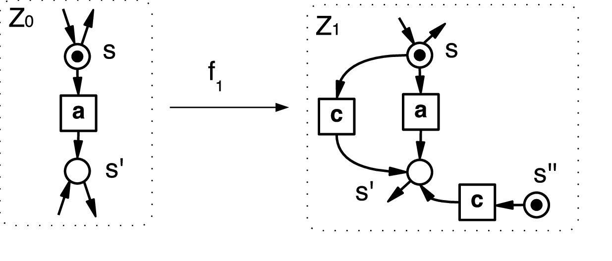
[open net] An open net is a pair $Z=(N_{Z},O_{Z})$ , consisting of a P/T Petri net $N_{Z}=(S_{Z},T_{Z},\sigma_{Z},\tau_{Z},\lambda_{Z})$ and a pair $O_{Z}=(O_{Z}^{+},O_{Z}^{-})\in\mathbf{2}^{S_{Z}}\times\mathbf{2}^{S_{Z}}$ , the sets of input open, respectively, output open places of the net. A marked open net is a pair $(Z,\hat{u})$ where $Z$ is an open net and $\hat{u}\in{S}_{Z}^{\oplus}$ is the initial marking. Hereafter, unless stated otherwise, all open nets will be assumed implicitly to be marked. An open net will be denoted simply by $Z$ and the corresponding initial marking by $\hat{u}$ . Subscripts carry over to the net components. The graphical representation for open nets is similar to that for standard nets. In addition, the fact that a place is input or output open is represented by an ingoing or outgoing dangling arc, respectively. For instance, in net $Z_{1}$ of Fig. 1, place $s$ is both input and output open, while $s^{\prime}$ is only output open.

Refer to caption — Figure 1. Two open nets and an open net morphism.

The notion of enabledness for transitions is the usual one, but besides the changes produced by the firing of the transitions of the net, we consider also the interaction with the environment which is modelled by events, denoted by $+_{s}$ or $-_{s}$ , which produce or consume a token in an open place $s$ . Such events corresponds to the pseudo-transitions of [43] and to the transition in the universal context of [29].

{defi}

[set of extended events] Let $Z$ be an open net. The set of extended events of $Z$ , denoted by $\bar{T}_{Z}$ and ranged over by $\epsilon$ is defined as

$\bar{T}_{Z}=T_{Z}\cup\{+_{s}:s\in O_{Z}^{+}\}\cup\{-_{s}:s\in O_{Z}^{-}\}$ .

Defining ${\rm Phys.~Rev.~E}[+_{s}]=0$ and ${+_{s}}{{}^{\bullet}}=s$ , and symmetrically, ${\rm Phys.~Rev.~E}[-_{s}]=s$ and ${-_{s}}{{}^{\bullet}}=0$ , the notion of pre- and post-set extends to multisets of extended events.

Given a marking $u\in{O_{Z}^{+}}^{\oplus}$ , we denote by $+_{u}$ the multiset $\bigoplus_{s\in O_{Z}^{+}}u(s)\cdot+_{s}$ . Similarly, $-_{u}=\bigoplus_{s\in O_{Z}^{-}}u(s)\cdot-_{s}$ for $u\in{O_{Z}^{-}}^{\oplus}$ .

{defi}

[firings and steps] Let $Z$ be an open net. A step in $Z$ consists of the execution of a multiset of (extended) events $A\in{\bar{T}}_{Z}^{\oplus}$ , i.e.,

$u\oplus{\rm Phys.~Rev.~E}[A]\ [\/{A}\/\rangle\ u\oplus{A}{{}^{\bullet}}$ .

A step is called a firing when $A$ consists of a single event, i.e., $A=\epsilon\in\bar{T}_{Z}$ . A firing can be (i) the execution of a transition $u\oplus{\rm Phys.~Rev.~E}[t]\ [\/{t}\/\rangle\ u\oplus{t}{{}^{\bullet}}$ , with $u\in{S}_{Z}^{\oplus}$ , $t\in T_{Z}$ ; (ii) the creation of a token by the environment $u\ [\/{+_{s}}\/\rangle\ u\oplus s$ , with $u\in{S}_{Z}^{\oplus}$ , $s\in O_{Z}^{+}$ ; (iii) the deletion of a token by the environment $u\oplus s\ [\/{-_{s}}\/\rangle\ u$ , with $u\in{S}_{Z}^{\oplus}$ , $s\in O_{Z}^{-}$ . A step is the execution of a multiset of transitions and interactions with the environment, of the kind $A\oplus-_{w}\oplus+_{v}$ for $A\in{T}_{Z}^{\oplus},w\in{O^{-}_{Z}}^{\oplus}$ and $v\in{O^{+}_{Z}}^{\oplus}$ .

We now introduce suitable morphisms relating open nets, which are morphisms between the underlying P/T nets, satisfying certain conditions on the open places and on the initial marking. In particular, given an injective morphism $f:Z_{1}\to Z_{2}$ , we can think of $N_{Z_{1}}$ as a subnet of $N_{Z_{2}}$ . In this case, we require that a place of $Z_{1}$ is input/output open in $Z_{2}$ only if it is so in $Z_{1}$ , and that a transition in $T_{Z_{2}}-T_{Z_{1}}$ can put/remove a token on/from a place of $Z_{1}$ only if that place is input/output open in $Z_{1}$ . Furthermore, any place of $Z_{1}$ must have the same number of tokens of its image in $Z_{2}$ . This is formalized by the following definition, which introduces general morphisms, possibly non-injective.

{defi}

[open net category] An open net morphism $f:Z_{1}\to Z_{2}$ is a Petri net morphism $f:N_{Z_{1}}\to N_{Z_{2}}$ such that, if we define $\mathsf{in}({f})=\{s\in S_{Z_{1}}:{\rm Phys.~Rev.~E}[f_{S}(s)]-f_{T}({\rm Phys.~Rev.~E}[s])\neq\emptyset\}$ and $\mathsf{out}({f})=\{s\in S_{Z_{1}}:{f_{S}(s)}{{}^{\bullet}}-f_{T}({s}{{}^{\bullet}})\neq\emptyset\}$ , then

(1)

(i) $f_{S}^{-1}(O_{Z_{2}}^{+})\cup\mathsf{in}({f})\subseteq O_{Z_{1}}^{+}$ and (ii) $f_{S}^{-1}(O_{Z_{2}}^{-})\cup\mathsf{out}({f})\subseteq O_{Z_{1}}^{-}$ .
(2)

$\hat{u}_{1}=({\hat{u}_{2}}\!\downarrow\!{f_{S}})$ (reflection of initial marking).

The morphism $f$ is called an open net embedding if both $f_{T}$ and $f_{S}$ are injective. We will denote by $\mathbf{ONet}$ the category of open nets and open net morphisms.

Conceptually, condition 1 formalizes the intuition that each open net can interact with the environment only through open places. In fact, given an embedding $f:Z_{1}\to Z_{2}$ , if $s$ is a place of $Z_{1}$ which is open in $Z_{2}$ , then an interaction of the environment with $Z_{2}$ through $s$ would also affect $Z_{1}$ : therefore $s$ must be open in $Z_{1}$ as well. That is, input/output open places must be reflected by the embedding, as stated by the first part of conditions 1.(i) and 1.(ii). Furthermore, if a transition in $T_{Z_{2}}-T_{Z_{1}}$ can put a token in a place $s$ of $Z_{1}$ , this is seen from $Z_{1}$ as an interaction with the environment, and therefore $s$ must be (input) open in $Z_{1}$ : this is formalized by the second part of conditions 1.(i) and 1.(ii). Finally, condition 2 requires the marking of $Z_{1}$ to be the projection of the marking of $Z_{2}$ : any place $s_{1}\in S_{Z_{1}}$ must carry the same number of tokens as its image $f(s_{1})\in S_{Z_{2}}$ , i.e., $\hat{u}_{1}(s_{1})=\hat{u}_{2}(f(s_{1}))$ for any $s_{1}\in S_{Z_{1}}$ .

Consider, for instance, morphism $f_{1}:Z_{0}\to Z_{1}$ in Fig. 1: the mapping of places and transitions is suggested by the shape and labelling of the nets. Note that in $Z_{1}$ a “new” $c$ -labelled transition is attached to the places $s$ and $s^{\prime}$ . This is legal since the corresponding places in $Z_{0}$ are output open and input open, respectively. Note also that the number of tokens in places in $Z_{0}$ and in their image through $f_{1}$ is the same. Instead, the number of tokens in the place $s^{\prime\prime}$ in $Z_{1}$ is not constrained since it is not in the image of $f_{1}$ : the place is marked, but $f_{1}$ would have been a legal morphism also if $s^{\prime\prime}$ were not marked.

It is worth observing that most of the constructions in the paper will be defined for open net embeddings, hence readers can limit their attention to embeddings if this helps the intuition. Still, on the formal side, working in a larger host category with more general morphisms is essential to obtain a characterisation of the composition operation in terms of pushouts. Specifically, non-injective open net morphisms are needed as mediating morphisms (recall, for example, that the category of sets with injective functions does not have all pushouts).

Observe that the constraints characterising open nets morphisms have an intuitive graphical interpretation:

$\bullet$

The connections of transitions to their pre-set and post-set have to be preserved. New connections cannot be added.
$\bullet$

In the larger net, a new arc may be attached to a place only if the corresponding place of the subnet has a dangling arc in the same direction. Dangling arcs may be removed, but cannot be added in the larger net.
$\bullet$

The number of tokens in each place in the source net must be preserved in the target. Instead, there are no restrictions on the marking of places of the target net which are not in the image of the source net.

In the sequel, given an open net morphism $f=\langle f_{S},f_{T}\rangle:Z_{1}\to Z_{2}$ , to lighten the notation we will omit the subscripts “ $S$ ” and “ $T$ ” in its place and transition components, writing $f(s)$ for $f_{S}(s)$ and $f(t)$ for $f_{T}(t)$ . Moreover we will write ${f}^{\oplus}:{\bar{T}}_{{Z_{1}}}^{\oplus}\to{\bar{T}}_{{Z_{2}}}^{\oplus}$ to denote the monoidal function defined on the generators by ${f}^{\oplus}(t)=f(t)$ for $t\in T_{Z_{1}}$ and, for $x\in\{+,-\}$ , ${f}^{\oplus}(x_{s})=x_{f(s)}$ , if $f(s)\in O_{Z_{2}}^{x}$ and ${f}^{\oplus}(x_{s})$ undefined, otherwise. Note that ${f}^{\oplus}$ can be partial since open places can be mapped to closed places.

The next proposition explicitly shows that category $\mathbf{ONet}$ , as introduced in Definition 1, is well defined. To prove this fact we will use the well-definedness of the category of unmarked open nets, introduced in [4]. This category, denoted here by $\mathbf{ONet}^{u}$ , has (unmarked) open nets as objects and mappings satisfying only condition 1 in Definition 1 as morphisms. These will be referred to as unmarked open net morphisms.

Proposition 1.

Open net morphisms are closed under composition.

Proof 1.1.

Let $f_{1}:Z_{1}\to Z_{2}$ and $f_{2}:Z_{2}\to Z_{3}$ be open net morphisms. Then $f_{1}$ and $f_{2}$ are unmarked open net morphisms and thus, since $\mathbf{ONet}^{u}$ is a well-defined category, also $f_{2}\circ f_{1}$ is an unmarked open net morphism. In order to prove that $f_{2}\circ f_{1}$ is a well defined open net morphism it remains to show that it satisfies also condition 2 in Definition 1, i.e., that it reflects the initial marking. But this fact follows easily from the definition. In fact, for any $s_{1}\in S_{Z_{1}}$ ,

$\hat{u}_{3}(f_{2}(f_{1}(s_{1})))=$

$=\hat{u}_{2}(f_{1}(s_{1}))$ [since $f_{2}$ is an open net morphism]

$=\hat{u}_{1}(s_{1})$ [since $f_{1}$ is an open net morphism] \qEd

$\hat{u}_{3}(f_{2}(f_{1}(s_{1})))=$
$=\hat{u}_{2}(f_{1}(s_{1}))$	[since $f_{2}$ is an open net morphism]
$=\hat{u}_{1}(s_{1})$	[since $f_{1}$ is an open net morphism] \qEd

Unlike most of the morphisms considered over Petri nets in the literature, open net morphisms are not simulations. As an example, consider the open net embedding in Fig. 2. While the transition labelled $c$ in the net $Z_{1}$ can fire infinitely many times, its image in the second net $Z_{2}$ can fire only once.

Instead, since open net embeddings are designed to capture the idea of inserting a net into a larger one, they are expected to reflect the behaviour, in the sense that given an embedding $f:Z_{0}\to Z_{1}$ , the behaviour of $Z_{1}$ can be projected along $f$ to the behaviour of $Z_{0}$ . The target net of a morphism is in general more “instantiated” and thus more constrained than the source net (e.g., a place which is open in the source net can be closed in the target). We will come back to this fact in the conclusions.

Although the paper will mainly use open net embeddings, a remark about non-injective morphisms is in order. Consider the open net morphism $f_{2}$ in Fig. 2, where $f_{2}(t^{\prime})=f_{2}(t^{\prime\prime})=t$ and $f_{2}(s^{\prime})=f_{2}(s^{\prime\prime})=s$ . As, intuitively, the two transitions of $Z_{1}$ become the same transition in $Z_{2}$ , in this case by reflection of behaviour we mean that the firing of $t$ in $Z_{2}$ must be reflected to the parallel firing of $t^{\prime}$ and $t^{\prime\prime}$ in $Z_{1}$ . Note that this is the case, e.g., for the initial markings: $s$ enables $t$ and its projection $({s}\!\downarrow\!{f_{2}})=s^{\prime}\oplus s^{\prime\prime}$ enables $t^{\prime}\oplus t^{\prime\prime}$ .

In the rest of this section we formalize the intuition that an open net embedding $f:Z\to Z^{\prime}$ reflects the behaviour by showing that each step of $Z^{\prime}$ can be projected along $f$ to a step of $Z$ . It could be shown that the behaviour of an open net is reflected along non-injective morphisms as well, but this would require some technical complications which we prefer to avoid, as it will not be used in the rest of the paper.

We start by defining the projection of multisets of extended events along open net embeddings.

{defi}

[projecting extended events] Given an open net embedding $f:Z\to Z^{\prime}$ , the projection of extended events along $f$ , denoted $({\_}\!\Downarrow\!{f}):\bar{T}_{Z^{\prime}}\to{\bar{T}}_{Z}^{\oplus}$ , is defined as follows. For each $\epsilon^{\prime}\in\bar{T}_{Z^{\prime}}$ ,

\bullet

if $\epsilon^{\prime}=t^{\prime}\in T_{Z^{\prime}}$ is a transition, then

({t^{\prime}}\!\Downarrow\!{f})=\begin{cases}t&\hbox{if $t\in T_{Z}$ and $f(t)=t^{\prime}$}\cr-_{({{\rm Phys.~Rev.~E}[t^{\prime}]}\!\downarrow\!{f})}\oplus+_{({{t^{\prime}}{{}^{\bullet}}}\!\downarrow\!{f})}&\hbox{if $t^{\prime}\not\in f(T_{Z})$}\end{cases}

$\bullet$

if $\epsilon^{\prime}=x_{s^{\prime}}$ , with $x\in\{+,-\}$ , then $({x_{s^{\prime}}}\!\Downarrow\!{f})=x_{({s^{\prime}}\!\downarrow\!{f})}$ .

The monoidal extension of $({\_}\!\Downarrow\!{f})$ to multisets of extended events will be denoted by the same symbol $({\_}\!\Downarrow\!{f}):{\bar{T}}_{{Z^{\prime}}}^{\oplus}\to{\bar{T}}_{Z}^{\oplus}$ .

In words, if we think of the embedding $f:Z\to Z^{\prime}$ as an inclusion, then given a transition $t^{\prime}$ , the projection $({t^{\prime}}\!\Downarrow\!{f})$ is the transition itself if $t^{\prime}$ is in $Z$ . Otherwise, if $t^{\prime}$ is not in $Z$ but it consumes or produces tokens in places of $Z$ , the projection of $t^{\prime}$ contains the corresponding extended events, expressing the interactions over open places. Similarly, the projection of an extended event $+_{s^{\prime}}$ is the event itself if $s^{\prime}$ is in $Z$ , and it is the empty multiset otherwise: in fact, in this case $({s^{\prime}}\!\downarrow\!{f})=0$ .

It is easily checked that the projection operation is well-defined, in the sense that, e.g., if $+_{s}\in({\epsilon}\!\Downarrow\!{f})$ then $s\in O_{Z}^{+}$ . In fact, if $+_{s}\in({t^{\prime}}\!\Downarrow\!{f})$ then $s\in\mathsf{in}({f})$ , while if $+_{s}\in({+_{s^{\prime}}}\!\Downarrow\!{f})$ , then $s^{\prime}\in O_{Z^{\prime}}^{+}$ and $f(s)=s^{\prime}$ . In both cases $s\in O_{Z}^{+}$ by condition 1.(i) of Definition 1.

The projections of multisets of places and extended events enjoy nice properties which are summarized by the next lemma.

Lemma 2 (properties of projection).

Let $f:Z\to Z^{\prime}$ be an open net embedding. Then

(1)

for $u_{1},u_{2}\in{S}_{{Z^{\prime}}}^{\oplus}$ we have

$({(u_{1}\oplus u_{2})}\!\downarrow\!{f})=({u_{1}}\!\downarrow\!{f})\oplus({u_{2}}\!\downarrow\!{f})\quad\hbox{and}\quad({0}\!\downarrow\!{f})=0$

and for $u\in{S}_{{Z}}^{\oplus}$

$({{f}^{\oplus}(u)}\!\downarrow\!{f})=u$
(2)

for $x_{1},x_{2}\in{\bar{T}}_{{Z^{\prime}}}^{\oplus}$ we have

$({(x_{1}\oplus x_{2})}\!\Downarrow\!{f})=({x_{1}}\!\Downarrow\!{f})\oplus({x_{2}}\!\Downarrow\!{f})\quad\hbox{and}\quad({0}\!\Downarrow\!{f})=0$

and for $x\in{\bar{T}}_{{Z}}^{\oplus}$ , if ${f}^{\oplus}(x)$ is defined we have

$({{f}^{\oplus}(x)}\!\Downarrow\!{f})=x$

(3)

given $A^{\prime}\in{\bar{T}}_{{Z^{\prime}}}^{\oplus}$

({{\rm Phys.~Rev.~E}[A^{\prime}]}\!\downarrow\!{f})={\rm Phys.~Rev.~E}[({A^{\prime}}\!\Downarrow\!{f})]\quad\hbox{and}\quad({{A^{\prime}}{{}^{\bullet}}}\!\downarrow\!{f})={({A^{\prime}}\!\Downarrow\!{f})}{{}^{\bullet}}

(4)

for $u\in{S}_{{Z^{\prime}}}^{\oplus}$ we have

${f}^{\oplus}(({u}\!\downarrow\!{f}))\leq u$

Proof 1.2.

Proofs are routine. We prove explicitly only the third point. Since ${\rm Phys.~Rev.~E}$ and ${(\cdot)}{{}^{\bullet}}$ are monoidal functions it is sufficient to prove the result only on the generators. We concentrate on ${\rm Phys.~Rev.~E}$ , since the proof for ${(\cdot)}{{}^{\bullet}}$ is completely analogous.

We distinguish various cases:

$\bullet$

$A^{\prime}=t^{\prime}\in T_{Z^{\prime}}$
If there exists $t\in T_{Z}$ such that $f(t)=t^{\prime}$ , then $({t^{\prime}}\!\Downarrow\!{f})=t$ . Since $f$ is an open net morphism ${f}^{\oplus}({\rm Phys.~Rev.~E}[t])={\rm Phys.~Rev.~E}[t^{\prime}]$ and thus, as desired

${\rm Phys.~Rev.~E}[({t^{\prime}}\!\Downarrow\!{f})]={\rm Phys.~Rev.~E}[t]=({{f}^{\oplus}({\rm Phys.~Rev.~E}[t])}\!\downarrow\!{f})=({{\rm Phys.~Rev.~E}[t^{\prime}]}\!\downarrow\!{f})$

where the second equality is justified by point (1).

If, instead, $t^{\prime}\not\in f(T_{Z})$ we have that $({t^{\prime}}\!\Downarrow\!{f})=-_{({{\rm Phys.~Rev.~E}[t^{\prime}]}\!\downarrow\!{f})}\oplus+_{({{t^{\prime}}{{}^{\bullet}}}\!\downarrow\!{f})}$ . Hence, in this case the result is obvious since

${\rm Phys.~Rev.~E}[({t^{\prime}}\!\Downarrow\!{f})]={\rm Phys.~Rev.~E}[(-_{({{\rm Phys.~Rev.~E}[t^{\prime}]}\!\downarrow\!{f})}\oplus+_{({{t^{\prime}}{{}^{\bullet}}}\!\downarrow\!{f})})]=({{\rm Phys.~Rev.~E}[t^{\prime}]}\!\downarrow\!{f})$
$\bullet$

$A^{\prime}=+_{s^{\prime}}$ or $A^{\prime}=-_{s^{\prime}}$
Suppose, e.g., that $A^{\prime}=-_{s^{\prime}}$ . In this case $({A^{\prime}}\!\Downarrow\!{f})=-_{({s^{\prime}}\!\downarrow\!{f})}$ and the result trivially holds.

We are now ready to present the main result of this section.

Lemma 3 (reflection of behaviour).

Let $f:Z\to Z^{\prime}$ be an open net embedding. For every step $u^{\prime}\ [\/{A^{\prime}}\/\rangle\ v^{\prime}$ in $Z^{\prime}$ there is a step $({u^{\prime}}\!\downarrow\!{f})\ [\/{({A^{\prime}}\!\Downarrow\!{f})}\/\rangle\ ({v^{\prime}}\!\downarrow\!{f})$ in $Z$ , called the projection of $u^{\prime}\ [\/{A^{\prime}}\/\rangle\ v^{\prime}$ along $f$ .

Proof 1.3.

Let $f:Z\to Z^{\prime}$ be an open net embedding and assume that $u^{\prime}\ [\/{A^{\prime}}\/\rangle\ v^{\prime}$ is a step in $Z^{\prime}$ . Therefore

$u^{\prime}=u^{\prime\prime}\oplus{\rm Phys.~Rev.~E}[A^{\prime}]$ and $v^{\prime}=u^{\prime\prime}\oplus{A}{{}^{\bullet}}$

Now, we have

$({u^{\prime}}\!\downarrow\!{f})=$

$=({u^{\prime\prime}}\!\downarrow\!{f})\oplus({{\rm Phys.~Rev.~E}[A^{\prime}]}\!\downarrow\!{f})$ [by Lemma 2.(1)]

$=({u^{\prime\prime}}\!\downarrow\!{f})\oplus{\rm Phys.~Rev.~E}[({A^{\prime}}\!\Downarrow\!{f})]$ [by Lemma 2.(3)]

$({u^{\prime}}\!\downarrow\!{f})=$
$=({u^{\prime\prime}}\!\downarrow\!{f})\oplus({{\rm Phys.~Rev.~E}[A^{\prime}]}\!\downarrow\!{f})$		[by Lemma 2.(1)]
$=({u^{\prime\prime}}\!\downarrow\!{f})\oplus{\rm Phys.~Rev.~E}[({A^{\prime}}\!\Downarrow\!{f})]$		[by Lemma 2.(3)]

and similarly

$({v^{\prime}}\!\downarrow\!{f})=({u^{\prime\prime}}\!\downarrow\!{f})\oplus{({A^{\prime}}\!\Downarrow\!{f})}{{}^{\bullet}}$

Therefore, as desired, there is the step

$({u^{\prime}}\!\downarrow\!{f})=({u^{\prime\prime}}\!\downarrow\!{f})\oplus{\rm Phys.~Rev.~E}[({A^{\prime}}\!\Downarrow\!{f})]\ [\/{({A^{\prime}}\!\Downarrow\!{f})}\/\rangle\ ({u^{\prime\prime}}\!\downarrow\!{f})\oplus{({A^{\prime}}\!\Downarrow\!{f})}{{}^{\bullet}}=({v^{\prime}}\!\downarrow\!{f})$ .

Observe that there is an obvious forgetful functor $\mathcal{F}:\mathbf{ONet}\to\mathbf{Net}$ , defined by $\mathcal{F}(Z)=N_{Z}$ and $\mathcal{F}(f:Z_{0}\to Z_{1})=f:N_{Z_{0}}\to N_{Z_{1}}$ . Since functor $\mathcal{F}$ acts on arrows as the identity, with abuse of notation, given an open net morphism $f:Z_{0}\to Z_{1}$ we will often write $f:\mathcal{F}(Z_{1})\to\mathcal{F}(Z_{2})$ instead of $\mathcal{F}(f):\mathcal{F}(Z_{1})\to\mathcal{F}(Z_{2})$ .

2. Composing Open Nets

We introduce next a basic mechanism for composing open nets which is characterised as a pushout construction in category $\mathbf{ONet}$ . A pushout is a canonical way of describing a gluing construction. The case of unmarked nets was already discussed in [4]. Here we extend the theory to deal with marked open nets. This will allow later to define reconfigurations of open nets, where the applicability of a reconfiguration rule can depend on the marking. Intuitively, two open nets $Z_{1}$ and $Z_{2}$ are composed by specifying a common subnet $Z_{0}$ , and then by joining the two nets along $Z_{0}$ .

Let us start with a technical definition which will be useful below.

Proposition 4 (composition of multisets).

Consider a pushout diagram in the category of sets as below, where all morphisms are injective.

Given $u_{1}\in{S}_{1}^{\oplus}$ and $u_{2}\in{S}_{2}^{\oplus}$ such that $({u_{1}}\!\downarrow\!{f_{1}})=({u_{2}}\!\downarrow\!{f_{2}})=u_{0}$ , there is a (unique) multiset $u_{3}\in{S}_{3}^{\oplus}$ such that $({u_{3}}\!\downarrow\!{\alpha_{i}})=u_{i}$ , for $i\in\{1,2\}$ . Such a multiset $u_{3}$ will be denoted by $u_{3}=u_{1}\uplus_{u_{0}}u_{2}$ or simply by $u_{1}\uplus u_{2}$ when making $u_{0}$ explicit is not needed.

Additionally, if $u_{3}=u_{1}\uplus_{u_{0}}u_{2}$ and $u_{3}^{\prime}=u_{1}^{\prime}\uplus_{u_{0}^{\prime}}u_{2}^{\prime}$ , then $u_{3}\oplus u_{3}^{\prime}=(u_{1}\oplus u_{1}^{\prime})\uplus_{(u_{0}\oplus u_{0}^{\prime})}(u_{2}\oplus u_{2}^{\prime})$ .

Proof 2.1.

Define $u_{3}\in{S}_{3}^{\oplus}$ as follows: for each $s\in S_{3}$ ,

$u_{3}(s)=\left\{\begin{array}[]{lll}u_{1}(s_{1})&&\text{if $\exists s_{1}\in S_{1}$ such that $\alpha_{1}(s_{1})=s$}\\ u_{2}(s_{2})&&\text{if $\exists s_{2}\in S_{2}$ such that $\alpha_{2}(s_{2})=s$}\end{array}\right.$

Let us start checking that $u_{3}$ is well-defined. In fact, firstly, the definition assigns a coefficient to every $s\in S_{3}$ because $\alpha_{1}$ and $\alpha_{2}$ are jointly surjective. Secondly, if there are $s_{1}\in S_{1}$ and $s_{2}\in S_{2}$ such that $\alpha_{1}(s_{1})=\alpha_{2}(s_{2})$ , since the square is a pushout and all functions are injective we have ${f_{1}}^{-1}(s_{1})=\{s_{0}\}$ and ${f_{2}}^{-1}(s_{2})=\{s_{0}\}$ for some $s_{0}\in S_{0}$ : thus, since $({u_{1}}\!\downarrow\!{f_{1}})=({u_{2}}\!\downarrow\!{f_{2}})$ by hypothesis, we obtain $u_{1}(s_{1})=u_{1}(f_{1}(s_{0}))=({u_{1}}\!\downarrow\!{f_{1}})(s_{0})=({u_{2}}\!\downarrow\!{f_{2}})(s_{0})=u_{2}(f_{2}(s_{0}))=u_{2}(s_{2})$ .

Now, in order to prove (for $i\in\{1,2\}$ ) that $({u_{3}}\!\downarrow\!{\alpha_{i}})=u_{i}$ , notice that, since $\alpha_{i}$ is injective, this amounts to show that for any $s\in S_{i}$ we have $u_{i}(s)=u_{3}(\alpha_{i}(s))$ , which is immediate by the definition of $u_{3}$ .

Concerning the second part of the statement, let $u_{3}=u_{1}\uplus_{u_{0}}u_{2}$ and $u_{3}^{\prime}=u_{1}^{\prime}\uplus_{u_{0}^{\prime}}u_{2}^{\prime}$ . Then just observe that by Lemma 2.(1), we have for $i\in\{1,2\}$

$({(u_{3}\oplus u_{3}^{\prime})}\!\downarrow\!{\alpha_{i}})=({u_{3}}\!\downarrow\!{\alpha_{i}})\oplus({u_{3}^{\prime}}\!\downarrow\!{\alpha_{i}})=u_{i}\oplus u^{\prime}_{i}$

hence the result $u_{3}\oplus u_{3}^{\prime}=(u_{1}\oplus u_{1}^{\prime})\uplus_{(u_{0}\oplus u_{0}^{\prime})}(u_{2}\oplus u_{2}^{\prime})$ follows by the defining property of the composition of markings.

Intuitively, the multiset $u_{1}\uplus_{u_{0}}u_{2}$ can be seen as the “least upper bound” of the images of the two multisets in ${S}_{3}^{\oplus}$ .

As in [3, 4], two embeddings $f_{1}:Z_{0}\to Z_{1}$ and $f_{2}:Z_{0}\to Z_{2}$ are called composable if the places which are used as interface by $f_{1}$ , i.e., the places $\mathsf{in}({f_{1}})$ and $\mathsf{out}({f_{1}})$ , are mapped by $f_{2}$ to input and output open places of $Z_{2}$ , respectively, and also the symmetric condition holds.

{defi}

[composability of embeddings] Let $f_{1}:Z_{0}\to Z_{1}$ , $f_{2}:Z_{0}\to Z_{2}$ be embeddings in $\mathbf{ONet}$ (see Fig. 3).We say that $f_{1}$ and $f_{2}$ are composable if

(1)

$f_{2}(\mathsf{in}({f_{1}}))\subseteq O_{Z_{2}}^{+}$ and $f_{2}(\mathsf{out}({f_{1}}))\subseteq O_{Z_{2}}^{-}$ ;
(2)

$f_{1}(\mathsf{in}({f_{2}}))\subseteq O_{Z_{1}}^{+}$ and $f_{1}(\mathsf{out}({f_{2}}))\subseteq O_{Z_{1}}^{-}$ .

Composability is necessary and sufficient to ensure that the pushout of $f_{1}$ and $f_{2}$ can be computed in $\mathbf{Net}$ and then lifted to $\mathbf{ONet}$ .

Proposition 5 (pushouts in $\mathbf{ONet}$ ).

Let $f_{1}:Z_{0}\to Z_{1}$ , $f_{2}:Z_{0}\to Z_{2}$ be embeddings in $\mathbf{ONet}$ (see Fig. 3). Compute the pushout of the corresponding diagram in category $\mathbf{Net}$ obtaining net $N_{Z_{3}}$ and morphisms $\alpha_{1}$ and $\alpha_{2}$ ,¹¹ 1 The pushout in $\mathbf{Net}$ is computed componentwise on places and transitions, by defining the pre- and post-set functions, for any $t_{i}\in T_{Z_{i}}$ , $i\in\{1,2\}$ , as $\sigma_{Z_{3}}(\alpha_{i}(t_{i}))={\alpha_{i}}^{\oplus}(\sigma_{Z_{i}}(t_{i}))$ and $\tau_{Z_{3}}(\alpha_{i}(t_{i}))={\alpha_{i}}^{\oplus}(\tau_{Z_{i}}(t_{i}))$ . It is routine to show that this definition is well given. and then take as open places, for $x\in\{+,-\}$ ,

$O_{Z_{3}}^{x}=\{s_{3}\in S_{Z_{3}}:\alpha_{1}^{-1}(s_{3})\subseteq O_{Z_{1}}^{x}\ \wedge\ \alpha_{2}^{-1}(s_{3})\subseteq O_{Z_{2}}^{x}\}$

and as initial marking $\hat{u}_{3}=\hat{u}_{1}\uplus_{\hat{u}_{0}}\hat{u}_{2}$ , defined according to Proposition 4. Then $(\alpha_{1},Z_{3},\alpha_{2})$ is the pushout in $\mathbf{ONet}$ of $f_{1}$ and $f_{2}$ if and only if $f_{1}$ and $f_{2}$ are composable. In this case we write $Z_{3}=Z_{1}+_{f_{1},f_{2}}Z_{2}$ .

Figure 3. Pushout in

\mathbf{ONet}

Proof 2.2.

We know by [4] (Proposition 6) that the above result holds for unmarked nets, i.e., in the category $\mathbf{ONet}^{u}$ . Here we must additionally show that (i) the $\alpha_{i}$ are marked morphisms and that (ii) if we take any other net $Z_{3}^{\prime}$ , with $\alpha_{i}^{\prime}:Z_{i}\to Z_{3}^{\prime}$ making the diagram commute, then the mediating morphism $\gamma:Z_{3}\to Z_{3}^{\prime}$ (which exists uniquely as an unmarked net morphism by the result in [4]) respects the condition on the marking.

Now, (i) is immediate since Proposition 4 tells us that $({\hat{u}_{3}}\!\downarrow\!{\alpha_{i}})=\hat{u}_{i}$ for $i\in\{1,2\}$ . Property (ii) can be proved along the same lines.

As an example, the open net embeddings $f_{1}$ and $f_{2}$ in Fig. 4 are composable. In fact, $\mathsf{in}({f_{1}})=\{s^{\prime}\}$ , $\mathsf{out}({f_{1}})=\{s\}$ and $\mathsf{in}({f_{2}})=\{s\}$ , $\mathsf{out}({f_{2}})=\{s^{\prime}\}$ , and thus it is easy to see that the conditions of Definition 2 are satisfied. The net $Z_{3}$ is the resulting pushout object.

3. Composing Steps

In this section we analyse the behaviour of an open net $Z_{3}$ arising as the composition of two nets $Z_{1}$ and $Z_{2}$ along an interface $Z_{0}$ . More specifically, we show that steps of the component nets $Z_{1}$ and $Z_{2}$ can be “composed” to give a step of $Z_{3}$ when they agree on the interface and satisfy suitable compatibility conditions.

For instance, concerning the example pushout in Fig. 4, note that net $Z_{1}$ can fire the transition labelled $a$ and the lower transition labelled $c$ . If this is “mimicked” in $Z_{2}$ by firing $a$ and putting a token into the lower place $s^{\prime}$ (via an interaction $+_{s^{\prime}}$ with the environment), then such steps are compatible in a sense made precise below and can be combined into a step of the composed net $Z_{3}$ .

We start with a technical lemma which will be pivotal in the paper. Assume that the first component makes a step and the second component imitates this step, acting only on the places of the common interface, without firing any internal transition. Then the two local steps can be combined to a step of the composed net.

Lemma 6.

Let $Z_{3}=Z_{1}+_{f_{1},f_{2}}Z_{2}$ be the pushout of two composable embeddings $f_{1}:Z_{0}\to Z_{1}$ and $f_{2}:Z_{0}\to Z_{2}$ in $\mathbf{ONet}$ (see Fig. 3). Let $u_{1}\ [\/{A_{1}}\/\rangle\ v_{1}$ and $u_{2}\ [\/{A_{2}}\/\rangle\ v_{2}$ be steps in $Z_{1}$ and $Z_{2}$ , respectively, such that $({u_{1}}\!\downarrow\!{f_{1}})=({u_{2}}\!\downarrow\!{f_{2}})$ and $A_{2}={f}_{2}^{\oplus}(({A_{1}}\!\Downarrow\!{f_{1}}))$ .

Then $({v_{1}}\!\downarrow\!{f_{1}})=({v_{2}}\!\downarrow\!{f_{2}})$ and, if we define $A_{3}={\alpha}_{1}^{\oplus}(A_{1})$ ,

$u_{1}\uplus u_{2}\ [\/{A_{3}}\/\rangle\ v_{1}\uplus v_{2}$ .

Proof 3.1.

Let us start showing that $A_{3}={\alpha}_{1}^{\oplus}(A_{1})$ is defined, i.e., that for $x\in\{+,-\}$ if $x_{s}\in A_{1}$ then $\alpha_{1}(s)\in O_{Z_{3}}^{x}$ . In fact $x_{s}\in A_{1}$ implies that $s\in O_{Z_{1}}^{x}$ ; now either $s\not\in f_{1}(S_{Z_{0}})$ and then $\alpha_{1}(s)\in O_{Z_{3}}^{x}$ by Proposition 5. Otherwise, since $f_{1}$ is an embedding, there is exactly one place in $S_{Z_{0}}$ which is mapped to $s$ . With a little abuse of notation let such place be denoted $f_{1}^{-1}(s)$ . Then clearly $f^{-1}_{1}(s)\in O_{Z_{0}}^{x}$ because $f_{1}$ is a morphism, and $f_{2}(f_{1}^{-1}(s))\in O_{Z_{2}}^{x}$ because ${f}_{2}^{\oplus}(({A_{1}}\!\Downarrow\!{f_{1}}))=A_{2}$ is defined by hypothesis; thus again $\alpha_{1}(s)\in O_{Z_{3}}^{x}$ by Proposition 5.

Next observe that, since $A_{2}={f}_{2}^{\oplus}(({A_{1}}\!\Downarrow\!{f_{1}}))$ is defined, by Lemma 2.(2),

$({A_{2}}\!\Downarrow\!{f_{2}})=({A_{1}}\!\Downarrow\!{f_{1}})$ .

Let $A_{0}=({A_{i}}\!\Downarrow\!{f_{i}})$ , for $i\in\{1,2\}$ , be the common projection. As a consequence, we have ${\rm Phys.~Rev.~E}[({A_{2}}\!\Downarrow\!{f_{2}})]={\rm Phys.~Rev.~E}[({A_{1}}\!\Downarrow\!{f_{1}})]$ and thus, by Lemma 2.(3)

$({{\rm Phys.~Rev.~E}[A_{1}]}\!\downarrow\!{f_{1}})$ = $({{\rm Phys.~Rev.~E}[A_{2}]}\!\downarrow\!{f_{2}})$

so that we can consider the composition of markings ${\rm Phys.~Rev.~E}[A_{1}]\uplus_{{\rm Phys.~Rev.~E}[A_{0}]}{\rm Phys.~Rev.~E}[A_{2}]$ . We claim that

{\rm Phys.~Rev.~E}[A_{3}]={\rm Phys.~Rev.~E}[A_{1}]\uplus_{{\rm Phys.~Rev.~E}[A_{0}]}{\rm Phys.~Rev.~E}[A_{2}]

(1)

and symmetrically, since $({{A_{1}}{{}^{\bullet}}}\!\downarrow\!{f_{1}})=({{A_{2}}{{}^{\bullet}}}\!\downarrow\!{f_{2}})$ , that

${A_{3}}{{}^{\bullet}}={A_{1}}{{}^{\bullet}}\uplus_{{A_{0}}{{}^{\bullet}}}{A_{2}}{{}^{\bullet}}$

Let us concentrate on ${\rm Phys.~Rev.~E}$ , as the other case is analogous. To prove (1), by Proposition 4 we can show that $({{\rm Phys.~Rev.~E}[A_{3}]}\!\downarrow\!{\alpha_{1}})={\rm Phys.~Rev.~E}[A_{1}]$ and $({{\rm Phys.~Rev.~E}[A_{3}]}\!\downarrow\!{\alpha_{2}})={\rm Phys.~Rev.~E}[A_{2}]$ . In fact we have

$({{\rm Phys.~Rev.~E}[A_{3}]}\!\downarrow\!{\alpha_{1}})=$

$={\rm Phys.~Rev.~E}[({A_{3}}\!\Downarrow\!{\alpha_{1}})]$ [by Lemma 2.(3)]

$={\rm Phys.~Rev.~E}[({{\alpha}_{1}^{\oplus}(A_{1})}\!\Downarrow\!{\alpha_{1}})]$ [by definition of $A_{3}$ ]

$={\rm Phys.~Rev.~E}[A_{1}]$ [by Lemma 2.(2)]

and

$({{\rm Phys.~Rev.~E}[A_{3}]}\!\downarrow\!{\alpha_{2}})=$

$={\rm Phys.~Rev.~E}[({A_{3}}\!\Downarrow\!{\alpha_{2}})]$ [by Lemma 2.(3)]

$={\rm Phys.~Rev.~E}[({{\alpha}_{1}^{\oplus}(A_{1})}\!\Downarrow\!{\alpha_{2}})]$ [by definition of $A_{3}$ ]

$({{\rm Phys.~Rev.~E}[A_{3}]}\!\downarrow\!{\alpha_{2}})=$
$={\rm Phys.~Rev.~E}[({A_{3}}\!\Downarrow\!{\alpha_{2}})]$		[by Lemma 2.(3)]
$={\rm Phys.~Rev.~E}[({{\alpha}_{1}^{\oplus}(A_{1})}\!\Downarrow\!{\alpha_{2}})]$		[by definition of $A_{3}$ ]

Thus to conclude we must show that ${\rm Phys.~Rev.~E}[({{\alpha}_{1}^{\oplus}(A_{1})}\!\Downarrow\!{\alpha_{2}})]={\rm Phys.~Rev.~E}[A_{2}]$ , and this is proved by showing

({{\alpha}_{1}^{\oplus}(A_{1})}\!\Downarrow\!{\alpha_{2}})={f}_{2}^{\oplus}(({A_{1}}\!\Downarrow\!{f_{1}}))[=A_{2}]

(2)

Since $({\_}\!\Downarrow\!{\_})$ is monoidal in the first argument by Lemma 2.(1), it is sufficient to show (2) on generators:

$\bullet$

$A_{1}=t_{1}$
We distinguish two subcases. If $({t_{1}}\!\Downarrow\!{f_{1}})=t_{0}\in T_{Z_{0}}$ then $A_{2}=f_{2}(t_{0})=({\alpha_{1}(t_{1})}\!\Downarrow\!{\alpha_{2}})$ , as desired, by construction of the pushout.

If, instead, $({t_{1}}\!\Downarrow\!{f_{1}})=-_{({{\rm Phys.~Rev.~E}[t_{1}]}\!\downarrow\!{f_{1}})}\oplus+_{({{t_{1}}{{}^{\bullet}}}\!\downarrow\!{f_{1}})}$ , then

$A_{2}=-_{{f}_{2}^{\oplus}(({{\rm Phys.~Rev.~E}[t_{1}]}\!\downarrow\!{f_{1}}))}\oplus+_{{f}_{2}^{\oplus}(({{t_{1}}{{}^{\bullet}}}\!\downarrow\!{f_{1}}))}$

On the other hand, we have

$({{\alpha}_{1}^{\oplus}(A_{1})}\!\Downarrow\!{\alpha_{2}})=({\alpha_{1}(t_{1})}\!\Downarrow\!{\alpha_{2}})=-_{({{\rm Phys.~Rev.~E}[\alpha_{1}(t_{1})]}\!\downarrow\!{\alpha_{2}})}\oplus+_{({{\alpha_{1}(t_{1})}{{}^{\bullet}}}\!\downarrow\!{\alpha_{2}})}$

Now, by exploiting the fact that $Z_{3}$ is a pushout, it is easy to see that ${f}_{2}^{\oplus}(({{\rm Phys.~Rev.~E}[t_{1}]}\!\downarrow\!{f_{1}}))=({{\rm Phys.~Rev.~E}[\alpha_{1}(t_{1})]}\!\downarrow\!{\alpha_{2}})$ and similarly ${f}_{2}^{\oplus}(({{t_{1}}{{}^{\bullet}}}\!\downarrow\!{f_{1}}))=({{\alpha_{1}(t_{1})}{{}^{\bullet}}}\!\downarrow\!{\alpha_{2}})$ . Hence we conclude that $A_{2}=({{\alpha}_{1}^{\oplus}(A_{1})}\!\Downarrow\!{\alpha_{2}})$ , as desired.
$\bullet$

$A_{1}=+_{s_{1}}$ or $A_{1}=-_{s_{1}}$
Assume, for instance, that $A_{1}=+_{s_{1}}$ (the other case is completely analogous). Therefore

$A_{2}={f}_{2}^{\oplus}(({A_{1}}\!\Downarrow\!{f_{1}}))=+_{{f}_{2}^{\oplus}(({s_{1}}\!\downarrow\!{f_{1}}))}$

On the other hand

$({{\alpha}_{1}^{\oplus}(A_{1})}\!\Downarrow\!{\alpha_{2}})=({+_{\alpha_{1}(s_{1})}}\!\Downarrow\!{\alpha_{2}})=+_{({\alpha_{1}(s_{1})}\!\downarrow\!{\alpha_{2}})}$

and, again, by the fact that $Z_{3}$ is a pushout, we deduce easily that ${f}_{2}^{\oplus}(({s_{1}}\!\downarrow\!{f_{1}}))=({\alpha_{1}(s_{1})}\!\downarrow\!{\alpha_{2}})$ , hence the desired equality.

This concludes the proof of (2), from which (1) follows.

Now, by exploiting (1) we can easily conclude. In fact, the steps in $Z_{1}$ and $Z_{2}$ are of the kind

$u_{i}=u_{i}^{\prime}\oplus{\rm Phys.~Rev.~E}[A_{i}]\ [\/{A_{i}}\/\rangle\ u_{i}^{\prime}\oplus{A_{i}}{{}^{\bullet}}=v_{i}$

for $i\in\{1,2\}$ . First observe that, since $({u_{1}}\!\downarrow\!{f_{1}})=({u_{2}}\!\downarrow\!{f_{2}})$ and $({{\rm Phys.~Rev.~E}[A_{1}]}\!\downarrow\!{f_{1}})=({{\rm Phys.~Rev.~E}[A_{2}]}\!\downarrow\!{f_{2}})$ , we immediately get:

$({u_{1}^{\prime}}\!\downarrow\!{f_{1}})=({u_{2}^{\prime}}\!\downarrow\!{f_{2}})$

Let $u_{0}^{\prime}=({u_{i}^{\prime}}\!\downarrow\!{f_{i}})$ , for $i\in\{1,2\}$ , be the common projection. Since $v_{i}=u_{i}^{\prime}\oplus{A_{i}}{{}^{\bullet}}$ , for $i\in\{1,2\}$ , by the fact that $({{A_{1}}{{}^{\bullet}}}\!\downarrow\!{f_{1}})=({{A_{2}}{{}^{\bullet}}}\!\downarrow\!{f_{2}})$ , we deduce that, as desired

$({v_{1}}\!\downarrow\!{f_{1}})=({v_{2}}\!\downarrow\!{f_{2}})$

Hence, if $v_{0}=({v_{i}}\!\downarrow\!{f_{i}})$ is the common projection, we can define $v_{3}=v_{1}\uplus_{v_{0}}v_{2}$ .

Now, if we set $u_{3}^{\prime}=u_{1}^{\prime}\uplus_{u_{0}^{\prime}}u_{2}^{\prime}$ we have

$u_{3}=u_{1}\uplus_{u_{0}}u_{2}=$

$=(u_{1}^{\prime}\oplus{\rm Phys.~Rev.~E}[A_{1}])\uplus_{u_{0}^{\prime}\oplus{\rm Phys.~Rev.~E}[A_{0}]}(u_{2}^{\prime}\oplus{\rm Phys.~Rev.~E}[A_{2}])=$

$=(u_{1}^{\prime}\uplus_{u_{0}^{\prime}}u_{2}^{\prime})\oplus({\rm Phys.~Rev.~E}[A_{1}]\uplus_{{\rm Phys.~Rev.~E}[A_{0}]}{\rm Phys.~Rev.~E}[A_{2}])=$ [by Proposition 4]

$=u_{3}^{\prime}\oplus{\rm Phys.~Rev.~E}[A_{3}]$ [by (1)]

$u_{3}=u_{1}\uplus_{u_{0}}u_{2}=$
$=(u_{1}^{\prime}\oplus{\rm Phys.~Rev.~E}[A_{1}])\uplus_{u_{0}^{\prime}\oplus{\rm Phys.~Rev.~E}[A_{0}]}(u_{2}^{\prime}\oplus{\rm Phys.~Rev.~E}[A_{2}])=$
$=(u_{1}^{\prime}\uplus_{u_{0}^{\prime}}u_{2}^{\prime})\oplus({\rm Phys.~Rev.~E}[A_{1}]\uplus_{{\rm Phys.~Rev.~E}[A_{0}]}{\rm Phys.~Rev.~E}[A_{2}])=$		[by Proposition 4]
$=u_{3}^{\prime}\oplus{\rm Phys.~Rev.~E}[A_{3}]$		[by (1)]

Therefore we have the step

$u_{3}\ [\/{A_{3}}\/\rangle\ u_{3}^{\prime}\oplus{A_{3}}{{}^{\bullet}}$ .

By a sequence of passages analogous to those used above, we can show that $u_{3}^{\prime}\oplus{A_{3}}{{}^{\bullet}}=v_{3}$ and thus, as desired, $u_{3}\ [\/{A_{3}}\/\rangle\ v_{3}$ .

The fact that such step projects to $u_{i}\ [\/{A_{i}}\/\rangle\ v_{i}$ for $i\in\{1,2\}$ immediately follows by construction.

We are now able to show how steps of the component nets can be “joined” to a step of their composition, provided that the steps satisfy a suitable compatibility condition, that we are going to introduce. Roughly, we must be able to split each of the two steps $A_{1},A_{2}$ into an internal part $A_{i}^{I}$ and an external part $A_{i}^{E}$ , with the intuition that the external part can include only firings of transitions in the interface and interactions with the environment induced by the internal part of the other step.

Put more precisely, from the point of view of $Z_{1}$ the events can be of four different kinds: (1) transitions that are local to $Z_{1}$ (2) transitions that occur also in $Z_{0}$ (3) interactions with $Z_{2}$ (of the form $+_{s},-_{s}$ ) (4) interactions with the environment of both nets (also of the form $+_{s},-_{s}$ ). Now if one splits the set $A_{1}$ into $A_{1}^{I}$ and $A_{1}^{E}$ , it is necessary to put all events of type (1) into $A_{1}^{I}$ and all events of type (3) into $A_{1}^{E}$ . For the remaining two types we have a choice, but whenever we put an event of $Z_{1}$ into $A_{1}^{E}$ , we have to put the corresponding event in $Z_{2}$ into $A_{2}^{I}$ (and vice versa).

For reasons of simplicity we have chosen to work with a split into only two sets instead of four, even if this split is non-unique.

{defi}

[compatible steps] Let $Z_{3}=Z_{1}+_{f_{1},f_{2}}Z_{2}$ be a pushout in $\mathbf{ONet}$ . We say that two steps $u_{i}\ [\/{A_{i}}\/\rangle\ v_{i}$ ( $i\in\{1,2\}$ ) are compatible if $({u_{1}}\!\downarrow\!{f_{1}})=({u_{2}}\!\downarrow\!{f_{2}})$ and we can decompose the steps as $A_{i}=A_{i}^{I}\oplus A_{i}^{E}$ ( $i\in\{1,2\}$ ) such that

$A_{2}^{E}={f}_{2}^{\oplus}(({A_{1}^{I}}\!\Downarrow\!{f_{1}}))$ and $A_{1}^{E}={f}_{1}^{\oplus}(({A_{2}^{I}}\!\Downarrow\!{f_{2}}))$

It is immediate to see that if $A_{1}$ and $A_{2}$ are compatible, then $({A_{1}}\!\Downarrow\!{f_{1}})=({A_{2}}\!\Downarrow\!{f_{2}})$ .

For instance, let us consider again the pushout in Fig. 4. Two compatible steps can be $A_{1}=t_{0}\oplus t_{1}^{\prime}$ and $A_{2}=t_{0}\oplus+_{s^{\prime}}$ . The compatibility is witnessed by the decomposition $A_{1}^{I}=A_{1}$ , $A_{1}^{E}=0$ and $A_{2}^{I}=0$ , $A_{2}^{E}=A_{2}$ . As mentioned above such decompositions are not uniquely determined: alternative ones are given by $A_{1}^{I}=t_{1}^{\prime}$ , $A_{1}^{E}=t_{0}$ and $A_{2}^{I}=t_{0}$ , $A_{2}^{E}=+_{s^{\prime}}$ . Note that since transition $t_{0}$ also belongs to the interface, it can be considered either internal to $Z_{1}$ or internal to $Z_{2}$ , while $t_{1}^{\prime}$ has to be considered internal to $Z_{1}$ , and the interaction $+_{s^{\prime}}$ on the open place $s^{\prime}$ has to be considered external to $Z_{2}$ .

Another simple example of compatible steps is given by $A_{1}=-_{s}$ and $A_{2}=-_{s}$ . In this case, we have the choice to consider the only event $-_{s}$ internal to $Z_{1}$ and external to $Z_{2}$ or vice versa.

Lemma 7 (composing steps).

Let $f_{1}:Z_{0}\to Z_{1}$ and $f_{2}:Z_{0}\to Z_{2}$ be composable embeddings in $\mathbf{ONet}$ and let $Z_{3}=Z_{1}+_{f_{1},f_{2}}Z_{2}$ . Let $u_{1}\ [\/{A_{1}}\/\rangle\ v_{1}$ and $u_{2}\ [\/{A_{2}}\/\rangle\ v_{2}$ be compatible steps and let $A_{i}=A_{i}^{I}\oplus A_{i}^{E}$ , for $i\in\{1,2\}$ , be a corresponding decomposition (see Definition 3). Then there exists a unique step $u_{3}\ [\/{A_{3}}\/\rangle\ v_{3}$ , with $A_{3}={\alpha}_{1}^{\oplus}(A_{1}^{I})\oplus{\alpha}_{2}^{\oplus}(A_{2}^{I})$ , which is projected to $u_{i}\ [\/{A_{i}}\/\rangle\ v_{i}$ along $\alpha_{i}$ for $i\in\{1,2\}$ .

Vice versa, any step $u_{3}\ [\/{A_{3}}\/\rangle\ v_{3}$ projects over two compatible steps $u_{1}\ [\/{({A_{3}}\!\Downarrow\!{\alpha_{1}})}\/\rangle\ v_{1}$ of $Z_{1}$ and $u_{2}\ [\/{({A_{3}}\!\Downarrow\!{\alpha_{2}})}\/\rangle\ v_{2}$ of $Z_{2}$ , whose composition gives back the original step.

Proof 3.2.

Concerning the first part, by definition of compatibility, we know that $A_{1}$ and $A_{2}$ can be decomposed as $A_{i}=A_{i}^{I}\oplus A_{i}^{E}$ ( $i\in\{1,2\}$ ) such that

$A_{2}^{E}={f}_{2}^{\oplus}(({A_{1}^{I}}\!\Downarrow\!{f_{1}}))$ and $A_{1}^{E}={f}_{1}^{\oplus}(({A_{2}^{I}}\!\Downarrow\!{f_{2}}))$ .

Moreover, $({u_{1}}\!\downarrow\!{f_{1}})=({u_{2}}\!\downarrow\!{f_{2}})$ .

Now, since $u_{i}\ [\/{A_{i}^{I}\oplus A_{i}^{E}}\/\rangle\ v_{i}$ , we can find markings $u_{i}^{I}$ , $u_{i}^{E}$ , $v_{i}^{I}$ , $v_{i}^{E}$ such that

$u_{1}^{I}\ [\/{A_{1}^{I}}\/\rangle\ v_{1}^{I}$ $u_{2}^{E}\ [\/{A_{2}^{E}}\/\rangle\ v_{2}^{E}$ , $({u_{1}^{I}}\!\downarrow\!{f_{1}})=({u_{2}^{E}}\!\downarrow\!{f_{2}})$

$u_{1}^{E}\ [\/{A_{1}^{E}}\/\rangle\ v_{1}^{E}$ , $u_{2}^{I}\ [\/{A_{2}^{I}}\/\rangle\ v_{2}^{I}$ , $({u_{1}^{E}}\!\downarrow\!{f_{1}})=({u_{2}^{I}}\!\downarrow\!{f_{2}})$

In fact, just observe that, since $u_{i}\ [\/{A_{i}}\/\rangle\ v_{i}$ , the marking $u_{i}$ must be of the kind $w_{i}\oplus{\rm Phys.~Rev.~E}[A_{i}^{I}]\oplus{\rm Phys.~Rev.~E}[A_{i}^{E}]$ and similarly $v_{i}=w_{i}\oplus{A_{i}^{I}}{{}^{\bullet}}\oplus{A_{i}^{E}}{{}^{\bullet}}$ . Thus we could choose

$u_{1}^{I}={\rm Phys.~Rev.~E}[A_{1}^{I}]$ , $v_{1}^{I}={A_{1}^{I}}{{}^{\bullet}}$ , $u_{2}^{E}={\rm Phys.~Rev.~E}[A_{2}^{E}]$ , $v_{2}^{E}={A_{2}^{E}}{{}^{\bullet}}$ ,

and dually

$u_{1}^{E}={\rm Phys.~Rev.~E}[A_{1}^{E}]\oplus w_{1}$ , $v_{1}^{E}={A_{1}^{E}}{{}^{\bullet}}\oplus w_{1}$ $u_{2}^{I}={\rm Phys.~Rev.~E}[A_{2}^{I}]\oplus w_{2}$ , $v_{2}^{I}={A_{2}^{I}}{{}^{\bullet}}\oplus w_{2}$

Therefore, we can use Lemma 6 and, defining $u_{3}^{\prime}=u_{1}^{I}\uplus u_{2}^{E}$ , $u_{3}^{\prime\prime}=u_{1}^{E}\uplus u_{2}^{I}$ , $v_{3}^{\prime}=v_{1}^{I}\uplus v_{2}^{I}$ , $v_{3}^{\prime\prime}=v_{1}^{E}\uplus v_{2}^{E}$ , we conclude

$u_{3}^{\prime}\ [\/{{\alpha}_{1}^{\oplus}(A_{1}^{I})}\/\rangle\ v_{3}^{\prime}$ and $u_{3}^{\prime\prime}\ [\/{{\alpha}_{2}^{\oplus}(A_{2}^{I})}\/\rangle\ v_{3}^{\prime\prime}$

Therefore

$u_{3}^{\prime}\oplus u_{3}^{\prime\prime}\ [\/{{\alpha}_{1}^{\oplus}(A_{1}^{I})\oplus{\alpha}_{2}^{\oplus}(A_{2}^{I})}\/\rangle\ v_{3}^{\prime}\oplus v_{3}^{\prime\prime}$

By exploiting Proposition 4, we easily see that $u_{3}^{\prime}\oplus u_{3}^{\prime\prime}=(u_{1}^{I}\oplus u_{1}^{E})\uplus(u_{2}^{E}\oplus u_{2}^{I})=u_{1}\uplus u_{2}$ , where $u_{0}$ denotes the common projection of $u_{1}$ and $u_{2}$ over $Z_{0}$ . Similarly, $v_{3}^{\prime}\oplus v_{3}^{\prime\prime}=v_{1}\uplus v_{2}$ and thus

$u_{1}\uplus u_{2}\ [\/{{\alpha}_{1}^{\oplus}(A_{1}^{I})\oplus{\alpha}_{2}^{\oplus}(A_{1}^{E})}\/\rangle\ v_{1}\uplus v_{2}$

is the desired step. The fact that it projects over the steps we started from in $Z_{1}$ and $Z_{2}$ follows by construction.

For the second part, consider any step $u_{3}\ [\/{A_{3}}\/\rangle\ v_{3}$ . Let $A_{1}=({A_{3}}\!\Downarrow\!{\alpha_{1}})$ and $A_{2}=({A_{3}}\!\Downarrow\!{\alpha_{2}})$ . Decompose $A_{3}$ as

$A_{3}=A_{3}^{1}\oplus A_{3}^{2}\oplus A_{3}^{0}\oplus A_{3}^{open}$

where $A_{3}^{j}$ , for $j\in\{1,2\}$ includes only transitions in $\alpha_{i}(T_{Z_{i}}-f_{i}(T_{Z_{0}}))$ , $A^{0}_{3}$ includes only transitions in $\alpha_{i}(f_{i}(T_{Z_{0}}))$ and finally $A_{3}^{open}$ includes only interactions with the environment.

Then, if we define

$A_{1}^{I}=({A_{3}^{1}}\!\Downarrow\!{\alpha_{1}})$ $A_{1}^{E}=A_{1}\ominus A_{1}^{I}$

$A_{2}^{I}=({(A_{3}^{2}\oplus A_{3}^{0}\oplus A_{3}^{open})}\!\Downarrow\!{\alpha_{2}})$ $A_{2}^{E}=A_{2}\ominus A_{2}^{I}$

it is easy to show that the decomposition satisfies the requirements in Definition 3, hence the two steps are compatible, and their composition is immediately seen to give back the original step.

Note that, in the decomposition of steps $A_{1}$ and $A_{2}$ considered in the proof above, all firings of transitions in the interface $Z_{0}$ are included in the internal part of $A_{2}$ , i.e., no such transition is included in $A_{1}^{I}$ . The possibility of having a decomposition with these properties will be useful later, in the proof of the congruence results.

4. Bisimilarity of Open Nets

In this section we study various notions of bisimilarity for open nets, proving that they are congruences with respect to the colimit-based composition operation. The considered behavioural equivalences will differ for the choice of the observations, which can be single firings or parallel steps. Additionally, we will consider weak forms of such equivalences, arising in the presence of unobservable actions.

4.1. A High Level View on the Congruence Results

A first step consists of defining suitable labelled transition systems (ltss) associated with an open net. Generally speaking, net transitions carry a label which is observed when they fire. Additionally, in the labelled transition systems we also observe what happens at the open places. This corresponds to observing the potential interactions with the surrounding environment, as open places act as gluing points in the composition operation, and it is pivotal for the mentioned congruence results.

Given an open net $Z$ , the labeled transition systems we shall consider will have all markings of the net, ${S}_{Z}^{\oplus}$ , as states, but they will differ concerning the transitions and their labels. For example, in the firing lts the transitions are generated by the firings of $Z$ , and correspondingly they are labelled over the set

$\Lambda_{Z}=\Lambda\cup\{+_{s}:s\in O_{Z}^{+}\}\cup\{-_{s}:s\in O_{Z}^{-}\}$ .

As discussed in the conclusions, the firing lts resembles the labelled transition system arising from the view of Petri nets as reactive systems in [26, 35]. Analogous ltss are also obtained in [43] with the use of pseudo-transitions and in [29] by inserting a net in a universal context.

Instead, in the step lts the transitions are generated by the steps of $Z$ , and they are labeled over ${\Lambda}_{Z}^{\oplus}$ . The corresponding notion of bisimilarity will capture, to some extent, the concurrency properties of the system (see, e.g., [44, 30]).

For notational convenience we extend the labelling function $\lambda_{Z}$ to the set of extended events $\bar{T}_{Z}$ , by defining $\lambda_{Z}(x)=x$ for $x\in\bar{T}_{Z}-T_{Z}$ (i.e., for $x=+_{s}$ or $x=-_{s}$ with $s\in S_{Z}$ ).

{defi}

[step and firing lts for an open net] The step lts associated to an open net $Z$ is the pair $\langle{S}_{Z}^{\oplus},\to_{\mathsf{S},Z}\rangle$ , where states are markings $u_{Z}\in{S}_{Z}^{\oplus}$ and the transition relation $\to_{\mathsf{S},Z}\,\subseteq{S}_{Z}^{\oplus}\times{\Lambda}_{Z}^{\oplus}\times{S}_{Z}^{\oplus}$ includes all transitions

u_{Z}\stackrel{{\scriptstyle{{\lambda}_{Z}^{\oplus}(A)}}}{{\longrightarrow}}_{\mathsf{S},Z}u_{Z}^{\prime}

for all markings $u_{Z},u_{Z}^{\prime}\in{S}_{Z}^{\oplus}$ and $A\in{\bar{T}_{Z}}^{\oplus}$ such that there is a step $u_{Z}\ [\/{A}\/\rangle\ u_{Z}^{\prime}$ in $Z$ . The firing lts $\langle{S}_{Z}^{\oplus},\to_{\mathsf{F},Z}\rangle$ is defined similarly: the transition relation $\to_{\mathsf{F},Z}\,\subseteq{S}_{Z}^{\oplus}\times\Lambda_{Z}\times{S}_{Z}^{\oplus}$ includes all transitions

u_{Z}\stackrel{{\scriptstyle{\lambda_{Z}(\epsilon)}}}{{\longrightarrow}}_{\mathsf{F},Z}u_{Z}^{\prime}

such that there is a firing $u_{Z}\ [\/{\epsilon}\/\rangle\ u_{Z}^{\prime}$ in $Z$ , with $\epsilon\in\bar{T}_{Z}$ .

As we have done above for the transition relations, in the sequel the subscripts “S” and “F” will be used for distinguishing notions based on the step and on the firing behaviour, respectively, of a net.

When observing the behaviour of a system, usually only a subset of events is considered visible. Here this is formalised by selecting a subset of labels representing internal firings, playing a role similar to $\tau$ -actions in process calculi, and then considering a corresponding notion of weak bisimilarity. Let $\Lambda_{\tau}\subseteq\Lambda$ be a subset of unobservable labels, fixed for the rest of the paper.

{defi}

[weak transition systems] For $\mathsf{x}\in\{\mathsf{S},\mathsf{F}\}$ we write $v\stackrel{{\scriptstyle{\ell}}}{{\leadsto}}_{\mathsf{x},Z}v^{\prime}$ if $v,v^{\prime}\in{S}_{Z}^{\oplus}$ are markings such that $v\stackrel{{\scriptstyle{\ell^{\prime}}}}{{\longrightarrow}}_{\mathsf{x},Z}v^{\prime}$ with $\ell=({\ell^{\prime}}\!\downarrow\!{(\Lambda-\Lambda_{\tau})})$ . Then the weak (step or firing) lts is defined by letting

$\bullet$

$v\stackrel{{\scriptstyle{0}}}{{\Longrightarrow}}_{\mathsf{x},Z}v^{\prime}$ whenever $v\stackrel{{\scriptstyle{0}}}{{\leadsto}}^{*}_{\mathsf{x},Z}v^{\prime}$ .
$\bullet$

$v\stackrel{{\scriptstyle{\ell}}}{{\Longrightarrow}}_{\mathsf{x},Z}v^{\prime}$ whenever $v\ \stackrel{{\scriptstyle{0}}}{{\leadsto}}^{*}_{\mathsf{x},Z}\ \stackrel{{\scriptstyle{\ell}}}{{\leadsto}}_{\mathsf{x},Z}\ \stackrel{{\scriptstyle{0}}}{{\leadsto}}^{*}_{\mathsf{x},Z}\ v^{\prime}$ $\ell\neq 0$ .

Transitions labelled with $0$ will be often referred to as $\tau$ -transitions or silent transitions.

Weak step and firing bisimilarity is now defined in a standard way, but note that when the set of unobservable labels is empty, this actually corresponds to strong bisimilarity. Only, in order to be able to relate the extended events of the two nets, we need to specify for each open place of one net which is the corresponding open place in the other net; therefore bisimulations between two nets are parametrised by a bijection between their open places. Given two open nets $Z_{1}$ and $Z_{2}$ a correspondence $\eta=\langle\eta^{+},\eta^{-}\rangle$ between $Z_{1}$ and $Z_{2}$ is a pair of bijections $\eta^{+}:O_{Z_{1}}^{+}\to O_{Z_{2}}^{+}$ and $\eta^{-}:O_{Z_{1}}^{-}\to O_{Z_{2}}^{-}$ . In order to simplify the notation, in the following, given an open place $s_{1}\in O_{Z_{1}}^{+}\cup O_{Z_{1}}^{-}$ we will write simply $\eta(s_{1})$ to denote its image through the appropriate component of $\eta$ , i.e., a correspondence $\eta=\langle\eta^{+},\eta^{-}\rangle$ will be identified with the function $\eta^{+}\cup\eta^{-}:O_{Z_{1}}^{+}\cup O_{Z_{1}}^{-}\to O_{Z_{2}}^{+}\cup O_{Z_{2}}^{-}$ .

{defi}

[(weak) step and firing bisimilarity] Let $Z_{1}$ , $Z_{2}$ be open nets and $\eta:O_{Z_{1}}\leftrightarrow O_{Z_{2}}$ be a correspondence between $Z_{1}$ and $Z_{2}$ . A (weak) $\eta$ - $\mathsf{x}$ -bisimulation (with $\mathsf{x}\in\{\mathsf{S},\mathsf{F}\}$ - $\mathsf{S}$ for step and $\mathsf{F}$ for firing) between $Z_{1}$ and $Z_{2}$ is a relation over markings $\mathcal{R}\subseteq{S}_{1}^{\oplus}\times{S}_{2}^{\oplus}$ such that if $(u_{1},u_{2})\in\mathcal{R}$ then

$\bullet$

if $u_{1}\stackrel{{\scriptstyle{\ell}}}{{\leadsto}}_{\mathsf{x},Z_{1}}u_{1}^{\prime}$ in $Z_{1}$ , then there exists $u_{2}^{\prime}$ such that $u_{2}\stackrel{{\scriptstyle{{\eta}^{\oplus}(\ell)}}}{{\Longrightarrow}}_{\mathsf{x},Z_{2}}u_{2}^{\prime}$ in $Z_{2}$ and $(u_{1}^{\prime},u_{2}^{\prime})\in\mathcal{R}$ ;
$\bullet$

the symmetric condition holds;

where $\eta(+_{s})=+_{\eta(s)}$ , $\eta(-_{s})=-_{\eta(s)}$ , and $\eta(\ell)=\ell$ for any $\ell\in\Lambda$ .

Two open nets $Z_{1}$ and $Z_{2}$ are (weakly) $\eta$ - $\mathsf{x}$ -bisimilar, denoted $Z_{1}\approx_{\eta}^{\mathsf{x}}Z_{2}$ , if $\eta:O_{Z_{1}}\leftrightarrow O_{Z_{2}}$ is a correspondence and there exists a (weak) $\eta$ -bisimulation $\mathcal{R}$ over $Z_{1}$ and $Z_{2}$ such that $(\hat{u}_{1},\hat{u}_{2})\in\mathcal{R}$ . We will say that $Z_{1}$ and $Z_{2}$ are (weakly) $\mathsf{x}$ -bisimilar, written $Z_{1}\approx^{\mathsf{x}}Z_{2}$ , if $Z_{1}\approx_{\eta}^{\mathsf{x}}Z_{2}$ for some correspondence $\eta$ . Clearly, step bisimilarity is finer than firing bisimilarity, i.e., if $Z_{1}\approx^{\mathsf{S}}Z_{2}$ then $Z_{1}\approx^{\mathsf{F}}Z_{2}$ .

Observe that in the definition of step bisimilarity, whenever $v\stackrel{{\scriptstyle{\ell}}}{{\Longrightarrow}}_{\mathsf{S},Z}v^{\prime}$ and thus $v\ \stackrel{{\scriptstyle{0}}}{{\leadsto}}^{*}_{\mathsf{S},Z}\ \stackrel{{\scriptstyle{\ell}}}{{\leadsto}}_{\mathsf{S},Z}\ \stackrel{{\scriptstyle{0}}}{{\leadsto}}^{*}_{\mathsf{S},Z}\ v^{\prime}$ , one can assume that the step inducing $\stackrel{{\scriptstyle{\ell}}}{{\leadsto}}_{\mathsf{S},Z}$ does not include any $\tau$ -transition (since, if this is not the case, the $\tau$ -transitions can be anticipated or postponed).

As an example, consider the open nets in Fig. 5, which can be seen as the representation of (part of) the booking process in a travel agency. The bookings of the flight (bookFlight) and of the hotel (bookHotel) are independent and could be performed in parallel. However, this is possible only for agency A (Fig. 5(a)), while in agency B (Fig. 5(b)), where a single person takes care of all bookings, the two actions will be executed sequentially. Now, it is easy to check that, assuming that only the actions bookFlight and bookHotel are visible, the two nets are firing bisimilar, but they are not step bisimilar. Hence, as already mentioned, step bisimilarity discriminates also according to the degree of parallelism that is possible in a computation.

As already mentioned, weak bisimilarity boils down to the notion of strong bisimilarity when all labels are observable, i.e., when $\Lambda_{\tau}=\emptyset$ . For convenience of the reader we make explicit the notion of strong bisimilarity.

{defi}

[strong bisimilarity] When $Z_{1}$ and $Z_{2}$ are weakly $\eta$ - $\mathsf{x}$ -bisimilar open nets, with $\Lambda_{\tau}=\emptyset$ we say that $Z_{1}$ and $Z_{2}$ are strongly $\eta$ - $\mathsf{x}$ -bisimilar and write $Z_{1}\sim_{\eta}^{\mathsf{x}}Z_{2}$ or simply $Z_{1}\sim^{\mathsf{x}}Z_{2}$ . Explicitly, a strong $\eta$ - $\mathsf{x}$ -bisimulation over $Z_{1}$ and $Z_{2}$ is a relation over their markings $\mathcal{R}\subseteq{S}_{1}^{\oplus}\times{S}_{2}^{\oplus}$ such that if $(u_{1},u_{2})\in\mathcal{R}$ then

$\bullet$

if $u_{1}\stackrel{{\scriptstyle{\ell}}}{{\longrightarrow}}_{\mathsf{x},Z_{1}}u_{1}^{\prime}$ in $Z_{1}$ , then there exists $u^{\prime}_{2}$ such that $u_{2}\stackrel{{\scriptstyle{\eta(\ell)}}}{{\longrightarrow}}_{\mathsf{x},Z_{2}}u_{2}^{\prime}$ in $Z_{2}$ and $(u_{1}^{\prime},u_{2}^{\prime})\in\mathcal{R}$ ;
$\bullet$

the symmetric condition holds.

We can finally state the congruence property for the considered behavioural equivalences with respect to the composition operation on open nets. The result will be proved separately for the various cases in the next subsection.

Figure 6. Pushouts in

\mathbf{ONet}

Theorem 8 (bisimilarity is a congruence).

Let $Z_{0}$ , $Z_{1}$ , $Z_{2}$ , $W_{2}$ be open nets. Let $Z_{2}\approx_{\eta}^{\mathsf{x}}W_{2}$ , for some correspondence $\eta$ and ${\mathsf{x}}\in\{\mathsf{S},\mathsf{F}\}$ . Consider the nets $Z_{3}=Z_{1}+_{f_{1},f_{2}}Z_{2}$ and $W_{3}=Z_{1}+_{f_{1},g_{2}}W_{2}$ , as in Fig. 6 where $f_{1}$ , $f_{2}$ and $g_{2}$ are embeddings, $f_{1}$ and $f_{2}$ are composable, and $f_{1}$ and $g_{2}$ are composable as well.

If $g_{2}|_{O_{0}}=\eta\circ(f_{2}|_{O_{0}})$ (i.e., $f_{2}$ and $g_{2}$ are consistent with $\eta$ on open places) then $Z_{3}\approx_{\eta^{\prime}}^{\mathsf{x}}W_{3}$ , where $\eta^{\prime}:O_{Z_{3}}\leftrightarrow O_{W_{3}}$ is the correspondence defined as follows: for all $s\in O_{Z_{3}}$ , $\eta^{\prime}(s)=\beta_{1}(s^{\prime})$ if $s=\alpha_{1}(s^{\prime})$ , and $\eta^{\prime}(s)=\beta_{2}(\eta(s^{\prime}))$ if $s=\alpha_{2}(s^{\prime})$ .

4.2. Proofs of the Congruence Results

In order to prove the congruence results it is convenient to proceed as follows: we first consider strong step bisimilarity which can be more easily handled than its weak variant. Next the proof of the congruence result for the weak variant can adapted from the strong case. Finally, as firing bisimulation can (almost) be considered as a special case of step bisimulation, the proof of the corresponding congruence result easily follows from that of step bisimilarity. It is worth stressing that the complexity of the proof is mainly due to the fact that we consider steps instead of single firings.

We start with a technical lemma which will play a central role later. It states that for given composable embeddings $f_{1}:Z_{0}\to Z_{1}$ and $f_{2}:Z_{0}\to Z_{2}$ , any step in $Z_{2}$ where interactions with the environment only occur on places which are open also in $Z_{1}+_{Z_{0}}Z_{2}$ , can be projected along $f_{2}$ to $Z_{0}$ and then simulated in $Z_{1}$ .

Lemma 9.

Let $f_{1}:Z_{0}\to Z_{1}$ and $f_{2}:Z_{0}\to Z_{2}$ be composable embeddings in $\mathbf{ONet}$ , let $Z_{3}=Z_{1}+_{f_{1},f_{2}}Z_{2}$ and let $u_{i}\in{S_{Z_{i}}}^{\oplus}$ ( $i\in\{1,2\}$ ) be markings such that $({u_{1}}\!\downarrow\!{f_{1}})=({u_{2}}\!\downarrow\!{f_{2}})$ . Let $u_{2}\ [\/{A_{2}}\/\rangle\ v_{2}$ be a step such that if $x_{s}\in A_{2}$ , for $x\in\{+,-\}$ then $\alpha_{2}(s)\in O_{Z_{3}}^{x}$ . Then $u_{1}\ [\/{{f}_{1}^{\oplus}(({A_{2}}\!\Downarrow\!{f_{2}}))}\/\rangle\ v_{1}$ and $u_{1}\uplus u_{2}\ [\/{{\alpha}_{2}^{\oplus}(A_{2})}\/\rangle\ v_{1}\uplus v_{2}$ .

Proof 4.1.

Let $A_{1}={f}_{1}^{\oplus}(({A_{2}}\!\Downarrow\!{f_{2}}))$ . First note that $A_{1}$ is well-defined, i.e., $A_{1}\in{\bar{T}}_{{Z_{1}}}^{\oplus}$ . For instance, let us show that if $+_{s_{1}}\in A_{1}$ then $s_{1}$ is input open, i.e., $s_{1}\in O_{Z_{1}}^{+}$ . By definition of $A_{1}$ we deduce that there is $+_{s_{0}}\in({A_{2}}\!\Downarrow\!{f_{2}})$ with $f_{1}(s_{0})=s_{1}$ . Now, by the assumptions on $A_{2}$ , there are two possibilities:

$\bullet$

$+_{s_{0}}\in({t_{2}}\!\Downarrow\!{f_{2}})$ with $t_{2}\in T_{Z_{2}}$
By the definition of projection for steps, this implies that $f_{2}(s_{0})\in{\rm Phys.~Rev.~E}[t_{2}]$ , with $t_{2}\not\in f_{2}(T_{Z_{0}})$ and thus $s_{0}\in\mathsf{in}({f_{2}})$ . Since $f_{1}$ and $f_{2}$ are composable, we have that $s_{1}=f_{1}(s_{0})\in f_{1}(\mathsf{in}({f_{2}}))\subseteq O_{Z_{1}}^{+}$ , as desired.
$\bullet$

$+_{s_{0}}\in({+_{s_{2}}}\!\Downarrow\!{f_{2}})$ with $\alpha_{2}(s_{2})\in O_{Z_{3}}^{+}$
Since the diagram in Fig. 3 commutes, we have that $\alpha_{1}(s_{1})=\alpha_{2}(s_{2})$ . Since $\alpha_{2}(s_{2})\in O_{Z_{3}}^{+}$ , by condition (1) in the definition of open net morphism (Definition 1), $s_{1}\in O_{Z_{1}}^{+}$ , as desired.

Now observe that

${\rm Phys.~Rev.~E}[A_{1}]={\rm Phys.~Rev.~E}[({f}_{1}^{\oplus}(({A_{2}}\!\Downarrow\!{f_{2}})))]$

$={f}_{1}^{\oplus}({\rm Phys.~Rev.~E}[({A_{2}}\!\Downarrow\!{f_{2}})])$ [by def. of open net morphism]

$={f}_{1}^{\oplus}(({{\rm Phys.~Rev.~E}[A_{2}]}\!\downarrow\!{f_{2}}))$ [by Lemma 2.(3)]

${\rm Phys.~Rev.~E}[A_{1}]={\rm Phys.~Rev.~E}[({f}_{1}^{\oplus}(({A_{2}}\!\Downarrow\!{f_{2}})))]$
$={f}_{1}^{\oplus}({\rm Phys.~Rev.~E}[({A_{2}}\!\Downarrow\!{f_{2}})])$	[by def. of open net morphism]
$={f}_{1}^{\oplus}(({{\rm Phys.~Rev.~E}[A_{2}]}\!\downarrow\!{f_{2}}))$	[by Lemma 2.(3)]

Since the step $u_{2}\ [\/{A_{2}}\/\rangle\ v_{2}$ is enabled, we know that ${\rm Phys.~Rev.~E}[A_{2}]\leq u_{2}$ , and thus

${\rm Phys.~Rev.~E}[A_{1}]={f}_{1}^{\oplus}(({{\rm Phys.~Rev.~E}[A_{2}]}\!\downarrow\!{f_{2}}))$

$\leq{f}_{1}^{\oplus}(({u_{2}}\!\downarrow\!{f_{2}}))$

$={f}_{1}^{\oplus}(({u_{1}}\!\downarrow\!{f_{1}}))$ [since $({u_{2}}\!\downarrow\!{f_{2}})=({u_{1}}\!\downarrow\!{f_{1}})$ ]

$\leq u_{1}$ [by Lemma 2.(4)]

Hence, the step $u_{1}\ [\/{A_{1}}\/\rangle\ v_{1}$ can be performed. Clearly, the two steps in $Z_{1}$ and $Z_{2}$ are compatible, and thus we conclude with Lemma 7.

4.2.1. Strong Step Bisimilarity

Theorem 10.

Strong step bisimilarity is a congruence.

Proof 4.2.

Let $Z_{0}$ , $Z_{1}$ , $Z_{2}$ , $W_{2}$ be open nets, with $Z_{2}\sim_{\eta}^{\mathsf{S}}W_{2}$ , for some correspondence $\eta$ . Let $Z_{3}=Z_{1}+_{f_{1},f_{2}}Z_{2}$ and $W_{3}=Z_{1}+_{f_{1},g_{2}}W_{2}$ , as in Fig. 6, where $f_{1}$ , $f_{2}$ and $g_{2}$ are embeddings, with $f_{1}$ , $f_{2}$ and $f_{1}$ , $g_{2}$ composable and $g_{2}|_{O_{Z_{0}}}=\eta\circ(f_{2}|_{O_{Z_{0}}})$ .

To simplify the notation, assume, without loss of generality, that all the morphisms in the diagrams of Fig. 6 are inclusions and $\eta=id$ . Hence $f_{2}|_{O_{Z_{0}}}=g_{2}|_{O_{Z_{0}}}$ .

Now let $\mathcal{R}$ be a $\eta$ - $\mathsf{S}$ -bisimulation over $Z_{2}$ and $W_{2}$ such that $(\hat{u}_{2},\hat{v}_{2})\in\mathcal{R}$ , which exists by hypothesis. Consider the relation $\mathcal{R}^{\prime}$ over $Z_{3}$ and $W_{3}$ defined as

$\mathcal{R}^{\prime}=\{(u_{1}\uplus_{u_{0}}u_{2},v_{1}\uplus_{v_{0}}v_{2}):(u_{2},v_{2})\in\mathcal{R}\ \land\ u_{1}\ominus u_{0}=v_{1}\ominus v_{0}\}$

The condition above on $u_{1}$ and $v_{1}$ means that the markings can differ, but only for the number of tokens in places of the interface net $Z_{0}$ (notice that the marking of $Z_{0}$ is completely determined by the marking of components $Z_{2}$ and $W_{2}$ ).

We claim that $\mathcal{R}^{\prime}$ is a $\eta^{\prime}$ - $\mathsf{S}$ -bisimulation over $Z_{3}$ and $W_{3}$ , where $\eta^{\prime}$ is again the identity on open places. Since, by the construction of the pushout, $(\hat{u}_{3},\hat{v}_{3})=(\hat{u}_{1}\uplus_{\hat{u}_{0}}\hat{u}_{2},\hat{u}_{1}\uplus_{\hat{u}_{0}}\hat{v}_{2})\in\mathcal{R}^{\prime}$ , this provides the desired result.

In order to prove that $\mathcal{R}^{\prime}$ is a $\eta^{\prime}$ - $\mathsf{S}$ -bisimulation, assume that $u_{3}\stackrel{{\scriptstyle{\ell}}}{{\longrightarrow}}_{\mathsf{S},Z_{3}}u_{3}^{\prime}$ . Therefore

$u_{3}\ [\/{A_{3}}\/\rangle\ u_{3}^{\prime}$ with $\ell={\lambda}_{Z_{3}}^{\oplus}(A_{3})$

and by Lemma 7 we can project the step $A_{3}$ over the components $Z_{1}$ and $Z_{2}$ thus getting for $i\in\{1,2\}$ the following steps in $Z_{i}$ :

u_{i}\ [\/{A_{i}}\/\rangle\ u_{i}^{\prime}

(3)

Since by the same lemma such steps are compatible, according to Definition 3, we can find partitions

$A_{i}=A_{i}^{I}\oplus A_{i}^{E}$ with $i\in\{1,2\}$

such that

A_{1}^{E}={f}_{1}^{\oplus}(({A_{2}^{I}}\!\Downarrow\!{f_{2}}))\qquad A_{2}^{E}={f}_{2}^{\oplus}(({A_{1}^{I}}\!\Downarrow\!{f_{1}}))

(4)

and

A_{3}={\alpha}_{1}^{\oplus}(A_{1}^{I})\oplus{\alpha}_{2}^{\oplus}(A_{2}^{I})

(5)

Additionally, as shown in the proof of Lemma 7, we can assume, w.l.o.g., that $A_{2}^{E}$ consists only of interactions with the environment, i.e., $A_{2}^{E}\in{\{x_{s}\mid x\in\{+,-\},\ s\in O_{Z_{2}}^{x}\}}^{\oplus}$ , or, equivalently, that $A_{1}^{I}$ does not contain firings of transitions of $Z_{0}$ .

Now, since $(u_{2},v_{2})\in\mathcal{R}$ , the step (3) of $Z_{2}$ can be simulated by $W_{2}$ , i.e., there is

v_{2}\ [\/{B_{2}}\/\rangle\ v_{2}^{\prime}

(6)

with ${\lambda}^{\oplus}(B_{2})={\lambda}^{\oplus}(A_{2})$ and $(u_{2}^{\prime},v_{2}^{\prime})\in\mathcal{R}$ .

We can now split $B_{2}$ in an “internal” and an “external” part, according to the splitting of $A_{1}$ , i.e., we define

B_{2}^{E}=A_{2}^{E}\qquad\qquad B_{2}^{I}=B_{2}\ominus B_{2}^{E}

(7)

Notice that we can legally define $B_{2}^{E}=A_{2}^{E}$ since $A_{2}^{E}$ consists only of interactions with the environment, which are necessarily also in $B_{2}$ since ${\lambda}^{\oplus}(B_{2})={\lambda}^{\oplus}(A_{2})$ (and recall that places in the interface have the same name in $Z_{2}$ and $W_{2}$ ).

Now, define

	$\displaystyle v_{2}^{I}={\rm Phys.~Rev.~E}[B_{2}^{I}]$		$\displaystyle{v_{2}^{I}}^{\prime}={B_{2}^{I}}{{}^{\bullet}}$		(8)
	$\displaystyle v_{2}^{E}=v_{2}\ominus v_{2}^{I}$		$\displaystyle{v_{2}^{E}}^{\prime}=v_{2}^{\prime}\ominus{v_{2}^{I}}^{\prime}$		(9)

and thus we have

v_{2}^{I}\ [\/{B_{2}^{I}}\/\rangle\ {v_{2}^{I}}^{\prime}

(10)

v_{2}^{E}\ [\/{B_{2}^{E}}\/\rangle\ {v_{2}^{E}}^{\prime}

(11)

Now, the idea is to construct a step in $W_{3}$ by using separately the internal part of the step in $W_{2}$ and the internal part of the step in $Z_{1}$ (which plays the role of a context).

In order to apply Lemma 9 to the step in (10), we note that if $+_{s}\in B_{2}^{I}$ then $s\in O_{W_{3}}^{+}$ (and the same holds for $-_{s}$ ). In fact, if $+_{s}\in B_{2}^{I}$ , then by construction of $B_{2}^{I}$ and since ${\lambda}^{\oplus}(A_{2})={\lambda}^{\oplus}(B_{2})$ , we must have $+_{s}\in A_{2}^{I}$ . Now, if $s\not\in Z_{0}$ then, given that $s\in O_{Z_{2}}^{+}$ we have that $s\in O_{Z_{3}}^{+}=O_{W_{3}}^{+}$ . Otherwise, if $s\in Z_{0}$ then, by (4), we have that ${f}_{1}^{\oplus}(({+_{s}}\!\downarrow\!{f_{2}}))=+_{s}\in A_{1}^{E}$ , thus $s\in O_{Z_{1}}^{+}$ , and hence $s\in O_{Z_{3}}^{+}=O_{W_{3}}^{+}$ .

Therefore if we define:

v_{1}^{E}={f}_{1}^{\oplus}(({v_{2}^{I}}\!\downarrow\!{g_{2}}))\qquad B_{1}^{E}={f}_{1}^{\oplus}(({B_{2}^{I}}\!\Downarrow\!{g_{2}}))

(12)

since clearly $({v_{1}^{E}}\!\downarrow\!{f_{1}})=({v_{2}^{I}}\!\downarrow\!{g_{2}})$ , we can apply Lemma 9 to deduce that

$v_{1}^{E}\ [\/{B_{1}^{E}}\/\rangle\ {v_{1}^{E}}^{\prime}$

and

v_{1}^{E}\uplus v_{2}^{I}\ [\/{{\beta_{2}}^{\oplus}(B_{2}^{I})}\/\rangle\ {v_{1}^{E}}^{\prime}\uplus{v_{2}^{I}}^{\prime}

(13)

Note that $v_{1}^{E}\leq v_{1}$ . In fact $v_{2}^{I}\leq v_{2}$ . Therefore $({v_{2}^{I}}\!\downarrow\!{g_{2}})\leq({v_{2}}\!\downarrow\!{g_{2}})$ and thus

$v_{1}^{E}={f}_{1}^{\oplus}(({v_{2}^{I}}\!\downarrow\!{g_{2}}))\leq{f}_{1}^{\oplus}(({v_{2}}\!\downarrow\!{g_{2}}))\leq v_{1}$

Let us now construct the other part of the step in $W_{3}$ , arising as the composition of an internal step in $Z_{1}$ and the external part of the step in $W_{2}$ . As mentioned before, since the component $Z_{1}$ plays the role of a context (it is the same in both composed nets) we can simply define:

B_{1}^{I}=A_{1}^{I}

(14)

If we let

v_{1}^{I}=v_{1}\ominus v_{1}^{E}

(15)

then we can see that

v_{1}^{I}\ [\/{B_{1}^{I}}\/\rangle\ {v_{1}^{I}}^{\prime}

(16)

We can show that indeed ${\rm Phys.~Rev.~E}[B_{1}^{I}]\leq v_{1}^{I}$ , with a long, but easy calculation. In fact, since $A_{1}^{I}=B_{1}^{I}$ by (14)

{\rm Phys.~Rev.~E}[B_{1}^{I}]={\rm Phys.~Rev.~E}[A_{1}^{I}]=({{\rm Phys.~Rev.~E}[A_{1}^{I}]}\!\downarrow\!{(S_{Z_{1}}-S_{Z_{0}})})\oplus({{\rm Phys.~Rev.~E}[A_{1}^{I}]}\!\downarrow\!{S_{Z_{0}}})

(17)

In the last expression, $({{\rm Phys.~Rev.~E}[A_{1}^{I}]}\!\downarrow\!{(S_{Z_{1}}-S_{Z_{0}})})$ and $({{\rm Phys.~Rev.~E}[A_{1}^{I}]}\!\downarrow\!{S_{Z_{0}}})$ stands for the projections along the inclusions of $S_{Z_{1}}-S_{Z_{0}}$ and $S_{Z_{0}}$ , respectively, into $S_{Z_{1}}$ . Now, let us consider the two summands separately. Concerning the first one:

$({{\rm Phys.~Rev.~E}[A_{1}^{I}]}\!\downarrow\!{(S_{Z_{1}}-S_{Z_{0}})})\leq u_{1}\ominus u_{0}=$ [since $A_{1}^{I}$ enabled in $u_{1}$ by (3)]

$=v_{1}\ominus v_{0}=$ [by construction of $\mathcal{R}^{\prime}$ ]

$=v_{1}\ominus{f}_{1}^{\oplus}(({v_{2}}\!\downarrow\!{g_{2}}))$

$({{\rm Phys.~Rev.~E}[A_{1}^{I}]}\!\downarrow\!{(S_{Z_{1}}-S_{Z_{0}})})\leq u_{1}\ominus u_{0}=$	[since $A_{1}^{I}$ enabled in $u_{1}$ by (3)]
$=v_{1}\ominus v_{0}=$	[by construction of $\mathcal{R}^{\prime}$ ]
$=v_{1}\ominus{f}_{1}^{\oplus}(({v_{2}}\!\downarrow\!{g_{2}}))$

Let us consider the second one:

$({{\rm Phys.~Rev.~E}[A_{1}^{I}]}\!\downarrow\!{S_{Z_{0}}})={f}_{1}^{\oplus}(({{\rm Phys.~Rev.~E}[A_{1}^{I}]}\!\downarrow\!{f_{1}}))=$

$={f}_{1}^{\oplus}(({{\rm Phys.~Rev.~E}[A_{2}^{E}]}\!\downarrow\!{f_{2}}))=$ [since $({A_{1}^{I}}\!\Downarrow\!{f_{1}})=({A_{2}^{E}}\!\Downarrow\!{f_{2}})$ by (4)]

$={f}_{1}^{\oplus}(({{\rm Phys.~Rev.~E}[B_{2}^{E}]}\!\downarrow\!{g_{2}}))\leq$ [by (7) and the fact that $g_{2}$ , $f_{2}$ agree on $O_{Z_{0}}$ ]

$\leq{f}_{1}^{\oplus}(({v_{2}^{E}}\!\downarrow\!{g_{2}}))$ [since by (11) ${\rm Phys.~Rev.~E}[B_{2}^{E}\ \leq v_{2}^{E}]$ ]

$({{\rm Phys.~Rev.~E}[A_{1}^{I}]}\!\downarrow\!{S_{Z_{0}}})={f}_{1}^{\oplus}(({{\rm Phys.~Rev.~E}[A_{1}^{I}]}\!\downarrow\!{f_{1}}))=$
$={f}_{1}^{\oplus}(({{\rm Phys.~Rev.~E}[A_{2}^{E}]}\!\downarrow\!{f_{2}}))=$	[since $({A_{1}^{I}}\!\Downarrow\!{f_{1}})=({A_{2}^{E}}\!\Downarrow\!{f_{2}})$ by (4)]
$={f}_{1}^{\oplus}(({{\rm Phys.~Rev.~E}[B_{2}^{E}]}\!\downarrow\!{g_{2}}))\leq$	[by (7) and the fact that $g_{2}$ , $f_{2}$ agree on $O_{Z_{0}}$ ]
$\leq{f}_{1}^{\oplus}(({v_{2}^{E}}\!\downarrow\!{g_{2}}))$	[since by (11) ${\rm Phys.~Rev.~E}[B_{2}^{E}\ \leq v_{2}^{E}]$ ]

Putting together the two summands, from (17) we have

${\rm Phys.~Rev.~E}[B_{1}^{I}]\leq v_{1}\ominus{f}_{1}^{\oplus}(({v_{2}}\!\downarrow\!{g_{2}}))\oplus{f}_{1}^{\oplus}(({v_{2}^{E}}\!\downarrow\!{g_{2}}))=$

$=v_{1}\ominus{f}_{1}^{\oplus}(({v_{2}\ominus v_{2}^{E}}\!\downarrow\!{g_{2}}))=$ [since $v_{2}^{E}\leq v_{2}$ and $f$ injective]

$=v_{1}\ominus{f}_{1}^{\oplus}(({v_{2}^{I}}\!\downarrow\!{g_{2}}))=$ [since $v_{2}^{I}=v_{2}\ominus v_{2}^{E}$ by (9)]

$=v_{1}\ominus v_{1}^{E}=$ [by (12)]

$=v_{1}^{I}$ [by (15)]

${\rm Phys.~Rev.~E}[B_{1}^{I}]\leq v_{1}\ominus{f}_{1}^{\oplus}(({v_{2}}\!\downarrow\!{g_{2}}))\oplus{f}_{1}^{\oplus}(({v_{2}^{E}}\!\downarrow\!{g_{2}}))=$
$=v_{1}\ominus{f}_{1}^{\oplus}(({v_{2}\ominus v_{2}^{E}}\!\downarrow\!{g_{2}}))=$	[since $v_{2}^{E}\leq v_{2}$ and $f$ injective]
$=v_{1}\ominus{f}_{1}^{\oplus}(({v_{2}^{I}}\!\downarrow\!{g_{2}}))=$	[since $v_{2}^{I}=v_{2}\ominus v_{2}^{E}$ by (9)]
$=v_{1}\ominus v_{1}^{E}=$	[by (12)]
$=v_{1}^{I}$	[by (15)]

In order to apply Lemma 9 to the step (16), we can prove that if $+_{s}\in B_{1}^{I}$ then $s\in O_{W_{3}}^{+}$ (and the same for $-_{s}$ ) as in the previous case. Additionally, we have

$({v_{1}^{I}}\!\downarrow\!{f_{1}})=({(v_{1}\ominus v_{1}^{E})}\!\downarrow\!{f_{1}})=$ [by def. of $v_{1}^{I}$ in (15)]

$=({v_{1}}\!\downarrow\!{f_{1}})\ominus({v_{1}^{E}}\!\downarrow\!{f_{1}})=$

$=({v_{2}}\!\downarrow\!{g_{2}})\ominus({v_{1}^{E}}\!\downarrow\!{f_{1}})=$ [since $({v_{1}}\!\downarrow\!{f_{1}})=({v_{2}}\!\downarrow\!{g_{2}})$ by hypothesis]

$=({v_{2}}\!\downarrow\!{g_{2}})\ominus({v_{2}^{I}}\!\downarrow\!{g_{2}})=$ [since $({v_{1}^{E}}\!\downarrow\!{f_{1}})=({v_{2}^{I}}\!\downarrow\!{g_{2}})$ by (12)]

$=({(v_{2}\ominus v_{2}^{I})}\!\downarrow\!{g_{2}})=$

$=({v_{2}^{E}}\!\downarrow\!{g_{2}})$ [by def. of $v_{2}^{E}$ in (9)]

$({v_{1}^{I}}\!\downarrow\!{f_{1}})=({(v_{1}\ominus v_{1}^{E})}\!\downarrow\!{f_{1}})=$	[by def. of $v_{1}^{I}$ in (15)]
$=({v_{1}}\!\downarrow\!{f_{1}})\ominus({v_{1}^{E}}\!\downarrow\!{f_{1}})=$
$=({v_{2}}\!\downarrow\!{g_{2}})\ominus({v_{1}^{E}}\!\downarrow\!{f_{1}})=$	[since $({v_{1}}\!\downarrow\!{f_{1}})=({v_{2}}\!\downarrow\!{g_{2}})$ by hypothesis]
$=({v_{2}}\!\downarrow\!{g_{2}})\ominus({v_{2}^{I}}\!\downarrow\!{g_{2}})=$	[since $({v_{1}^{E}}\!\downarrow\!{f_{1}})=({v_{2}^{I}}\!\downarrow\!{g_{2}})$ by (12)]
$=({(v_{2}\ominus v_{2}^{I})}\!\downarrow\!{g_{2}})=$
$=({v_{2}^{E}}\!\downarrow\!{g_{2}})$	[by def. of $v_{2}^{E}$ in (9)]

and moreover

$B_{2}^{E}={g_{2}}^{\oplus}(({B_{1}^{I}}\!\Downarrow\!{f_{1}}))$ .

In fact

$B_{2}^{E}=A_{2}^{E}$ [by (7)]

$={f}_{2}^{\oplus}(({A_{1}^{I}}\!\Downarrow\!{f_{1}}))=$ [by (4)]

$={f}_{2}^{\oplus}(({B_{1}^{I}}\!\Downarrow\!{f_{1}}))=$ [by (14)]

$={g_{2}}^{\oplus}(({B_{1}^{I}}\!\Downarrow\!{f_{1}}))=$ [since $g_{2}$ and $f_{2}$ “agree” on $O_{Z_{0}}$ ]

Therefore, by Lemma 9, we have that

v_{2}^{E}\ [\/{B_{2}^{E}}\/\rangle\ {v_{2}^{E}}^{\prime}

(18)

and

v_{1}^{I}\uplus v_{2}^{E}\ [\/{{\beta_{1}}^{\oplus}(B_{1}^{I})}\/\rangle\ {v_{1}^{I}}^{\prime}\uplus{v_{2}^{E}}^{\prime}

(19)

Now, by Proposition 4, we can join the steps (13) and (19) and obtain

$(v_{1}^{E}\uplus v_{2}^{I})\oplus(v_{1}^{I}\uplus v_{2}^{E})\ [\/{{\beta_{1}}^{\oplus}(B_{1}^{I})\oplus{\beta_{2}}^{\oplus}(B_{2}^{I})}\/\rangle\ ({v_{1}^{I}}^{\prime}\uplus{v_{2}^{E}}^{\prime})\oplus({v_{1}^{E}}^{\prime}\uplus{v_{2}^{I}}^{\prime})$

i.e., the desired step which can be used to simulate $u_{3}\stackrel{{\scriptstyle{\ell}}}{{\longrightarrow}}_{\mathsf{S},Z_{3}}u_{3}^{\prime}$ . In fact the label is

${\lambda}_{{W_{3}}}^{\oplus}({\beta_{1}}^{\oplus}(B_{1}^{I})\oplus{\beta_{2}}^{\oplus}(B_{2}^{I}))=$

= ${\lambda}_{{W_{3}}}^{\oplus}({\beta_{1}}^{\oplus}(B_{1}^{I}))\oplus{\lambda}_{{W_{3}}}^{\oplus}({\beta_{2}}^{\oplus}(B_{2}^{I}))$ [since the diagram in Fig. 6 commutes]

= ${\lambda}_{{Z_{1}}}^{\oplus}(B_{1}^{I})\oplus{\lambda}_{{W_{2}}}^{\oplus}(B_{2}^{I})$ [since $A_{1}^{I}=B_{1}^{I}$ by (14) and

${\lambda}_{{W_{2}}}^{\oplus}(B_{2}^{I})={\lambda}_{{Z_{2}}}^{\oplus}(A_{2}^{I})$ by construction (6)]

= ${\lambda}_{{Z_{1}}}^{\oplus}(A_{1}^{I})\oplus{\lambda}_{{Z_{2}}}^{\oplus}(A_{2}^{I})$ [since the diagram in Fig. 6 commutes]

= ${\lambda}_{{Z_{3}}}^{\oplus}({\alpha}_{1}^{\oplus}(A_{1}^{I}))\oplus{\lambda}_{{Z_{3}}}^{\oplus}({\alpha}_{2}^{\oplus}(A_{2}^{I}))$

= ${\lambda}_{{Z_{3}}}^{\oplus}({\alpha}_{1}^{\oplus}(A_{1}^{I})\oplus{\alpha}_{2}^{\oplus}(A_{2}^{I}))$ [by (5)]

= ${\lambda}_{{Z_{3}}}^{\oplus}(A_{3})$

$=\ell$

${\lambda}_{{W_{3}}}^{\oplus}({\beta_{1}}^{\oplus}(B_{1}^{I})\oplus{\beta_{2}}^{\oplus}(B_{2}^{I}))=$
= ${\lambda}_{{W_{3}}}^{\oplus}({\beta_{1}}^{\oplus}(B_{1}^{I}))\oplus{\lambda}_{{W_{3}}}^{\oplus}({\beta_{2}}^{\oplus}(B_{2}^{I}))$	[since the diagram in Fig. 6 commutes]
= ${\lambda}_{{Z_{1}}}^{\oplus}(B_{1}^{I})\oplus{\lambda}_{{W_{2}}}^{\oplus}(B_{2}^{I})$	[since $A_{1}^{I}=B_{1}^{I}$ by (14) and
	${\lambda}_{{W_{2}}}^{\oplus}(B_{2}^{I})={\lambda}_{{Z_{2}}}^{\oplus}(A_{2}^{I})$ by construction (6)]
= ${\lambda}_{{Z_{1}}}^{\oplus}(A_{1}^{I})\oplus{\lambda}_{{Z_{2}}}^{\oplus}(A_{2}^{I})$	[since the diagram in Fig. 6 commutes]
= ${\lambda}_{{Z_{3}}}^{\oplus}({\alpha}_{1}^{\oplus}(A_{1}^{I}))\oplus{\lambda}_{{Z_{3}}}^{\oplus}({\alpha}_{2}^{\oplus}(A_{2}^{I}))$
= ${\lambda}_{{Z_{3}}}^{\oplus}({\alpha}_{1}^{\oplus}(A_{1}^{I})\oplus{\alpha}_{2}^{\oplus}(A_{2}^{I}))$	[by (5)]
= ${\lambda}_{{Z_{3}}}^{\oplus}(A_{3})$
$=\ell$

Moreover, using (9), we have

$(v_{1}^{E}\uplus v_{2}^{I})\oplus(v_{1}^{I}\uplus v_{2}^{E})=(v_{1}^{I}\oplus v_{1}^{E})\uplus(v_{2}^{I}\oplus v_{2}^{E})=v_{1}\uplus v_{2}=v_{3}$ .

And, if we define

$v_{1}^{\prime}={v_{1}^{I}}^{\prime}\oplus{v_{1}^{E}}^{\prime}$

recalling that, by (9), $v_{2}^{\prime}={v_{2}^{I}}^{\prime}\oplus{v_{2}^{E}}^{\prime}$ , we have that the target state of the step is

$v_{3}^{\prime}=v_{1}^{\prime}\uplus v_{2}^{\prime}$

Now, $(u_{2}^{\prime},v_{2}^{\prime})\in\mathcal{R}$ by construction. Moreover, the fact that $u_{1}^{\prime}\ominus u_{0}^{\prime}=v_{1}^{\prime}\ominus v_{0}^{\prime}$ immediately follows from the fact that this property holds of the starting markings and we executed the same internal step in $Z_{1}$ .

Hence $(u_{3}^{\prime},v_{3}^{\prime})\in\mathcal{R}^{\prime}$ as desired.

4.2.2. Weak Step Bisimilarity

Theorem 11.

Weak step bisimilarity is a congruence.

Proof 4.3.

In order to show the desired result, we build on the proof of the strong case (Theorem 10). Let us use the same notation and define the relation $\mathcal{R}^{\prime}$ in the same way. In order to prove that $\mathcal{R}^{\prime}$ is an $\mathsf{S}$ -weak bisimulation we proceed as follows.

Let $u_{3}\stackrel{{\scriptstyle{\ell_{3}}}}{{\leadsto}}_{\mathsf{S},Z_{3}}u_{3}^{\prime}$ and let us focus on the case $\ell_{3}\neq 0$ (the case in which $\ell_{3}=0$ is completely analogous). This transition is induced by a step $u_{3}\ [\/{A_{3}}\/\rangle\ u_{3}^{\prime}$ , which can be projected over $Z_{1}$ and $Z_{2}$ , thus getting, for $i\in\{1,2\}$

$u_{i}\ [\/{A_{i}}\/\rangle\ u_{i}^{\prime}$

Now, since $(u_{2},v_{2})\in\mathcal{R}$ , the transition $u_{2}\stackrel{{\scriptstyle{\ell_{2}}}}{{\leadsto}}_{\mathsf{S},Z_{2}}u_{2}^{\prime}$ , induced by $u_{2}\ [\/{A_{2}}\/\rangle\ u_{2}^{\prime}$ can be simulated in $W_{2}$ , by $v\stackrel{{\scriptstyle{\ell_{2}}}}{{\Longrightarrow}}_{\mathsf{S},W_{2}}v^{\prime}$ . Let the weak transition in $W_{2}$ arise from the sequence of steps

$v_{2}=v_{2}^{0}\ [\/{B_{2}^{1}}\/\rangle\ v_{2}^{1}\ldots v_{2}^{h}\ [\/{B_{2}^{h}}\/\rangle\ v_{2}^{h+1}\ldots v_{2}^{k}\ [\/{B_{2}^{k}}\/\rangle\ v_{2}^{k+1}=v_{2}^{\prime}$

where ${\lambda}_{{W_{2}}}^{\oplus}(B_{2}^{i})=0$ for $i\neq h$ and ${\lambda}_{{W_{2}}}^{\oplus}(B_{2}^{h})=\ell$ (and as remarked after Definition 4.1 we can assume that no transition in $B_{2}^{h}$ has an unobservable label).

Now, any $\tau$ -step $v_{2}^{i}\ [\/{B_{2}^{i}}\/\rangle\ v_{2}^{i+1}$ ( $i<h$ ) consists only of firings of transitions of $W_{2}$ . Hence, as in the strong case, by using Lemma 9 we can conclude that there is a “corresponding” step $v_{1}^{i}\ [\/{B_{1}^{i}}\/\rangle\ v_{1}^{i+1}$ , consisting only of interactions with the environment, and their composition is a $\tau$ -step in $W_{3}$ of the kind $v_{1}^{i}\ [\/{{\alpha}_{2}^{\oplus}(B_{2}^{i})}\/\rangle\ v_{3}^{i+1}$ , with ${\lambda}_{{Z_{1}}}^{\oplus}(B_{1}^{i})=0$ .

Note that since $v_{1}^{i}\ [\/{B_{1}^{i}}\/\rangle\ v_{1}^{i+1}$ consists only of interactions with the environment, $u_{1}\ominus u_{0}=v_{1}^{i+1}\ominus v_{0}^{i+1}$ for $i<h$ .

For the “visible” step $v_{2}^{h}\ [\/{B_{2}^{h}}\/\rangle\ v_{2}^{h+1}$ , we can apply the same argument as in the strong case, to get steps $v_{1}^{h}\ [\/{B_{1}^{h}}\/\rangle\ v_{1}^{h+1}$ and $v_{3}^{h}\ [\/{B_{3}^{h}}\/\rangle\ v_{3}^{h+1}$ , with ${\lambda}_{{W_{3}}}^{\oplus}(B_{3}^{h})=\ell$ . Additionally, $u_{1}^{\prime}\ominus u_{0}^{\prime}=v_{1}^{h+1}\ominus v_{0}^{h+1}$ .

Repeating the same argument for the remaining $\tau$ -steps, $v_{2}^{i}\ [\/{B_{2}^{i}}\/\rangle\ v_{2}^{i+1}$ ( $i>h$ ), i.e., using again Lemma 9, we can prove that there are steps $v_{1}^{i}\ [\/{B_{1}^{i}}\/\rangle\ v_{1}^{i+1}$ , consisting only of interactions with the environment, correspondingly $\tau$ -steps in $W_{3}$ of the kind $v_{1}^{i}\ [\/{{\alpha}_{2}^{\oplus}(B_{2}^{i})}\/\rangle\ v_{3}^{i+1}$ , with ${\lambda}_{{Z_{1}}}^{\oplus}(B_{1}^{i})=0$ , for $i>h$ . Such sequence of further $\tau$ -steps in $W_{3}$ leads to a marking $v_{3}^{\prime}=v_{1}^{k+1}\uplus v_{2}^{k+1}$ , where $v_{1}^{k+1}\ominus v_{0}^{k+1}=u_{1}^{\prime}\ominus u_{0}^{\prime}$ and $v_{2}^{k+1}=v_{2}^{\prime}$ with $(u_{2}^{\prime},v_{2}^{\prime})\in\mathcal{R}$ . Hence $(u_{3}^{\prime},v_{3}^{\prime})\in\mathcal{R}^{\prime}$ .

In other words $v_{3}\stackrel{{\scriptstyle{\ell}}}{{\Longrightarrow}}_{\mathsf{S},W_{3}}v_{3}^{\prime}$ and $(u_{3}^{\prime},v_{3}^{\prime})\in\mathcal{R}^{\prime}$ , as desired.

4.2.3. Weak (and Strong) Firing Bisimilarity

Theorem 12.

Strong and weak firing bisimilarity are congruences.

Proof 4.4.

The proof remains essentially the same as for step bisimulation (Theorem 10 and Theorem 11). Only some minor adaptations are required.

Let us focus on weak bisimulation, which is the more general case. We use the same notation as in Theorem 11 and define $\mathcal{R}^{\prime}$ in the same way. In order to prove that $\mathcal{R}^{\prime}$ is an $\mathsf{S}$ -weak bisimulation we proceed as follows.

Let $(u_{3},v_{3})\in\mathcal{R}^{\prime}$ and let $u_{3}\stackrel{{\scriptstyle{\ell}}}{{\leadsto}}_{\mathsf{F},Z_{3}}u_{3}^{\prime}$ . Then there must be a step

$u_{3}\ [\/{\epsilon_{3}}\/\rangle\ u_{3}^{\prime}$

such that $\epsilon_{3}\in\bar{T}_{Z_{3}}$ and $\lambda_{Z_{3}}(\epsilon_{3})=\ell$ . We can project the step over $Z_{2}$ , thus getting

u_{2}\ [\/{A_{2}}\/\rangle\ u_{2}^{\prime}

(20)

The delicate case is the one in which $\epsilon_{3}=t_{3}\in T_{Z_{3}}-\alpha_{2}(T_{Z_{2}})$ . In fact, in this case, $A_{2}$ is in general a proper multiset (of interactions with the environment) and thus we cannot argue, as in the case of step bisimulation, that the transition $u_{2}\stackrel{{\scriptstyle{{\lambda}_{{Z_{2}}}^{\oplus}(A_{2})}}}{{\longrightarrow}}_{\mathsf{F},Z_{2}}u_{2}^{\prime}$ must be simulated by $W_{2}$ , since only single firings are simulated.

In order to proceed, we have first to linearise the step in (20) as

u_{2}\stackrel{{\scriptstyle{-_{s_{1}}}}}{{\longrightarrow}}_{\mathsf{F},Z_{2}}\ldots\stackrel{{\scriptstyle{-_{s_{k}}}}}{{\longrightarrow}}_{\mathsf{F},Z_{2}}\stackrel{{\scriptstyle{+_{s_{k+1}}}}}{{\longrightarrow}}_{\mathsf{F},Z_{2}}\ldots\stackrel{{\scriptstyle{+_{s_{k+h}}}}}{{\longrightarrow}}_{\mathsf{F},Z_{2}}u_{2}^{\prime}

(21)

Interestingly, the joint effect of the projection and of the linearization corresponds to the function $\psi$ used in [43, page 96] to project a firing in the combined net to a firing sequence in the host net. Now we can say that this is simulated in $W_{2}$ by

$v_{2}\stackrel{{\scriptstyle{-_{s_{1}}}}}{{\Longrightarrow}}_{\mathsf{F},W_{2}}\ldots\stackrel{{\scriptstyle{-_{s_{k}}}}}{{\Longrightarrow}}_{\mathsf{F},W_{2}}\stackrel{{\scriptstyle{+_{s_{k+1}}}}}{{\Longrightarrow}}_{\mathsf{F},W_{2}}\ldots\stackrel{{\scriptstyle{+_{s_{k+h}}}}}{{\Longrightarrow}}_{\mathsf{F},W_{2}}v_{2}^{\prime}$

namely

$v_{2}\stackrel{{\scriptstyle{0}}}{{\Longrightarrow}}_{\mathsf{F},W_{2}}\stackrel{{\scriptstyle{-_{s_{1}}}}}{{\longrightarrow}}_{\mathsf{F},W_{2}}\stackrel{{\scriptstyle{0}}}{{\Longrightarrow}}_{\mathsf{F},W_{2}}\ldots$
$\ldots\stackrel{{\scriptstyle{0}}}{{\Longrightarrow}}_{\mathsf{F},W_{2}}\stackrel{{\scriptstyle{-_{s_{k}}}}}{{\longrightarrow}}_{\mathsf{F},W_{2}}\stackrel{{\scriptstyle{0}}}{{\Longrightarrow}}_{\mathsf{F},W_{2}}\stackrel{{\scriptstyle{0}}}{{\Longrightarrow}}_{\mathsf{F},W_{2}}\stackrel{{\scriptstyle{+_{s_{k+1}}}}}{{\longrightarrow}}_{\mathsf{F},W_{2}}\stackrel{{\scriptstyle{0}}}{{\Longrightarrow}}_{\mathsf{F},W_{2}}$ …
$\ldots\stackrel{{\scriptstyle{0}}}{{\Longrightarrow}}_{\mathsf{F},W_{2}}\stackrel{{\scriptstyle{+_{s_{k+h}}}}}{{\longrightarrow}}_{\mathsf{F},W_{2}}\stackrel{{\scriptstyle{0}}}{{\Longrightarrow}}_{\mathsf{F},W_{2}}v_{2}^{\prime}$

which in turn (since $-_{s_{i}}$ and $+_{s_{j}}$ firings can be clearly postponed and anticipated, respectively) can be reorganised as

$v_{2}\stackrel{{\scriptstyle{0}}}{{\Longrightarrow}}_{\mathsf{F},W_{2}}\stackrel{{\scriptstyle{-_{s_{1}}}}}{{\longrightarrow}}_{\mathsf{F},W_{2}}\ldots\stackrel{{\scriptstyle{-_{s_{k}}}}}{{\longrightarrow}}_{\mathsf{F},W_{2}}\stackrel{{\scriptstyle{+_{s_{k+1}}}}}{{\longrightarrow}}_{\mathsf{F},W_{2}}\ldots\stackrel{{\scriptstyle{+_{s_{k+h}}}}}{{\longrightarrow}}_{\mathsf{F},W_{2}}\stackrel{{\scriptstyle{0}}}{{\Longrightarrow}}_{\mathsf{F},W_{2}}v_{2}^{\prime}$

and thus finally to

$v_{2}\stackrel{{\scriptstyle{0}}}{{\Longrightarrow}}_{\mathsf{F},W_{2}}\stackrel{{\scriptstyle{\ell_{2}}}}{{\Longrightarrow}}_{\mathsf{F},W_{2}}\stackrel{{\scriptstyle{0}}}{{\Longrightarrow}}_{\mathsf{F},W_{2}}v_{2}^{\prime}$

where $\ell_{2}=(\bigoplus_{i=1}^{k}+_{s_{1}})\oplus(\bigoplus_{i=1}^{h}-_{s_{i}})$ . Then we can proceed exactly as in the proof for step bisimilarity.

4.3. Comparison to CCS

We now give some hints as to why weak (firing) bisimilarity is a congruence in the case of open nets, but not in CCS [25]. Remember that a classical counterexample for CCS is as follows: $p_{1}=\tau.a.0\approx a.0=p_{2}$ , but $q_{1}=\tau.a.0+b.0\not\approx a.0+b.0=q_{2}$ . The reason for the latter inequality is that $q_{1}$ can do a $\tau$ and become $a.0$ , while $q_{2}$ cannot mimic this step.

Fig. 7 shows a similar situation of nondeterministic choice for open nets, where $\tau$ is the only unobservable label. However, note that here the two nets $Z_{1}$ (corresponding to $\tau.a.0$ ) and $Z_{1}^{\prime}$ (corresponding to $a.0$ ) are not weakly firing bisimilar. Whenever the $\tau$ -transition is fired in $Z_{1}$ , resulting in the marking $m_{1}$ , this can not be mimicked in $Z_{1}^{\prime}$ by staying idle, since then in $Z_{1}^{\prime}$ a transition with label $-_{s^{\prime}_{1}}$ is possible, while a transition labelled $-_{s_{1}}$ is not possible for the net $Z_{1}$ with marking $m_{1}$ . Also note that the places $s_{1}$ respectively $s^{\prime}_{1}$ must be output open in order to allow composition with the net $Z_{2}$ .

Roughly, this means that for open nets we are always able to observe the first invisible action in an open component, which is reminiscent of the definition of observation congruence in CCS: two processes $p,q$ are called observation congruent if they are weakly bisimilar, with the additional constraint that whenever the first step of $p$ is a $\tau$ -action, then it has to be answered by at least one $\tau$ -action of $q$ (and vice versa). In both settings it is only the first $\tau$ -action that can be observed but not the subsequent ones.

5. Some Proof Techniques for Bisimilarity

We next present some properties of (strong and weak) bisimilarity, which can help in bisimilarity proofs. We first show that the set of open places can be uniformly reduced without altering the equivalence of open nets. Then we provide an up-to technique for firing bisimilarity.

We start by showing that given two bisimilar nets, if we “close” corresponding open places in both nets we still get two bisimilar nets. Given an open net $Z$ and an open place $s\in O_{Z}^{x}$ , let us denote by $Z-(s,x)$ the open net obtained from $Z$ by closing place $s$ , i.e., $Z^{\prime}=(N,O_{Z^{\prime}})$ , where $O_{Z^{\prime}}^{x}=O_{Z}^{x}-\{s\}$ . The initial marking remains the same.

Proposition 13 (“closing” open places).

Let $Z_{1}\approx_{\eta}^{\mathsf{x}}Z_{2}$ , with $\mathsf{x}\in\{\mathsf{F},\mathsf{S}\}$ . Let $s\in O_{Z_{1}}^{x}$ ( $x\in\{-,+\}$ ) be an open place in $Z_{1}$ . Then the nets $Z_{1}-(s,x)$ and $Z_{2}-(\eta(s),x)$ are $\eta$ - $\mathsf{x}$ -bisimilar.

Proof 5.1.

Let $Z_{1}^{\prime}=Z_{1}-(s,x)$ and $Z_{2}^{\prime}=Z_{2}-(\eta(s),x)$ . Let $\mathcal{R}\subseteq{S}_{1}^{\oplus}\times{S}_{2}^{\oplus}$ be an $\eta$ - $\mathsf{x}$ -bisimulation such that $(\hat{u}_{1},\hat{u}_{2})\in\mathcal{R}$ . Then $\mathcal{R}$ is a bisimulation between $Z_{1}^{\prime}$ and $Z_{2}^{\prime}$ . In fact, if $(u_{1},u_{2})\in\mathcal{R}$ and $u_{1}\stackrel{{\scriptstyle{\ell}}}{{\leadsto}}_{\mathsf{x},Z_{1}^{\prime}}u_{1}^{\prime}$ then clearly $u_{1}\stackrel{{\scriptstyle{\ell}}}{{\leadsto}}_{\mathsf{x},Z_{1}}u_{1}^{\prime}$ . Since $\mathcal{R}$ is a bisimulation for $Z_{1}$ and $Z_{2}$ this implies that $u_{2}\stackrel{{\scriptstyle{\eta(\ell)}}}{{\Longrightarrow}}_{\mathsf{x},Z_{2}}u_{2}^{\prime}$ with $(u_{1}^{\prime},u_{2}^{\prime})\in\mathcal{R}$ . Since $\ell$ is a label in $Z_{1}^{\prime}$ where place $s$ has been closed, we are sure that $x_{s}\not\in\ell$ , and thus $u_{2}\stackrel{{\scriptstyle{\eta(\ell)}}}{{\Longrightarrow}}_{\mathsf{x},Z_{2}}u_{2}^{\prime}$ implies $u_{2}\stackrel{{\scriptstyle{\eta(\ell)}}}{{\Longrightarrow}}_{\mathsf{x},Z_{2}^{\prime}}u_{2}^{\prime}$ . Hence we get the desired result.

We next provide a kind of up-to technique for firing bisimilarity. Given an open net $Z$ , let us define the out-degree of a place $s\in S$ as the maximum number of tokens that the firing of an extended event can remove from $s$ , formally:

$deg({s})=\max\left(\{({\rm Phys.~Rev.~E}[t])(s):t\in T_{Z}\}\cup\{1:s\in O_{Z}^{-}\}\right)$

The idea, formalised by the notion of up-to bisimulation, is to allow tokens to be removed from input open places, when they exceed the out-degree of the place. More precisely, given a net $Z$ and a marking $u\in{S}^{\oplus}$ , let us say that a marking $v\in{O_{Z}^{+}}^{\oplus}$ is subtractable from $u$ if $\forall s\in O_{Z}^{+}.\ v(s)\leq\max\{u(s)-deg({s}),0\}$ . Note that when the number of tokens in a place $s$ does not exceed its out-degree, i.e., $u(s)\leq deg({s})$ , then $v(s)=0$ , i.e., no token is subtractable from $s$ . If instead, $u(s)>deg({s})$ , then the tokens in $s$ which exceeds the out-degree of $s$ can be safely subtracted from $s$ . It is clear that when $v$ is subtractable from $u$ , all transitions enabled in $u$ are also enabled in $u\ominus v$ . Note that the empty marking is subtractable from any other marking.

{defi}

[up-to firing bisimulation] Let $Z_{1}$ and $Z_{2}$ be open nets, and let $\eta:O_{Z_{1}}\leftrightarrow O_{Z_{2}}$ be a correspondence between $Z_{1}$ and $Z_{2}$ . A relation $\mathcal{R}\subseteq{S}_{1}^{\oplus}\times{S}_{2}^{\oplus}$ between markings is called an up-to $\eta$ - $\mathsf{F}$ -bisimulation if whenever $(u_{1},u_{2})\in\mathcal{R}$ then

$\bullet$

if $u_{1}\stackrel{{\scriptstyle{\ell}}}{{\leadsto}}_{\mathsf{F},Z_{1}}u_{1}^{\prime}$ , then there exist markings $u_{2}^{\prime}$ such that $u_{2}\stackrel{{\scriptstyle{\eta(\ell)}}}{{\Longrightarrow}}_{\mathsf{F},Z_{2}}u_{2}^{\prime}$ , and $v_{1}\in{O_{Z_{1}}^{+}}^{\oplus}$ subtractable from $u_{1}^{\prime}$ , with $(u_{1}^{\prime}\ominus v_{1},u_{2}^{\prime}\ominus{\eta}^{\oplus}(v_{1}))\in\mathcal{R}$ ;
$\bullet$

the symmetric condition holds.

That is, the intuition behind up-to bisimulations is that some tokens might be superfluous since they are not necessary to fire a transition. Hence in the bisimulation game they can be removed in the two successor markings.

A first technical lemma shows an invariance property of up-to $\mathsf{F}$ -bisimulations, with respect to adding tokens in open places.

Lemma 14.

Let $Z_{1}$ and $Z_{2}$ be open nets, let $\eta:O_{Z_{1}}\leftrightarrow O_{Z_{2}}$ be a correspondence between $Z_{1}$ and $Z_{2}$ , and let $\mathcal{R}$ be an up-to $\eta$ - $\mathsf{F}$ -bisimulation between $Z_{1}$ and $Z_{2}$ . Then

(1)

given any $s\in O_{Z_{1}}^{+}$ , the relation $\mathcal{R}^{s}=\mathcal{R}\cup\{(u_{1}\oplus s,u_{2}\oplus\eta(s)):(u_{1},u_{2})\in\mathcal{R}\}$ is an up-to $\eta$ - $\mathsf{F}$ -bisimulation.
(2)

$\mathcal{R}^{\prime}=\mathcal{R}\cup\{(u_{1}\oplus v_{1},u_{2}\oplus{\eta}^{\oplus}(v_{1})):(u_{1},u_{2})\in\mathcal{R}\ \wedge\ v_{1}\in{O_{Z_{1}}^{+}}^{\oplus}\}$ is an up-to $\eta$ - $\mathsf{F}$ -bisimulation.

Proof 5.2.

1. In order to simplify the notation, let us assume, without loss of generality, that $\eta$ is the identity (i.e., $O_{Z_{1}}^{+}=O_{Z_{2}}^{+}$ and $O_{Z_{1}}^{-}=O_{Z_{2}}^{-}$ ).

Let $(u_{1}\oplus s,u_{2}\oplus s)\in\mathcal{R}^{s}$ . Let us show that if $u_{1}\oplus s\stackrel{{\scriptstyle{\ell}}}{{\leadsto}}_{\mathsf{F},Z_{1}}u_{1}^{\prime}$ then there exists $u_{2}\oplus s\stackrel{{\scriptstyle{\ell}}}{{\Longrightarrow}}_{\mathsf{F},Z_{2}}u_{2}^{\prime}$ and $v\in O_{Z_{1}}^{+}$ subtractable from $u_{1}^{\prime}$ with $(u_{1}^{\prime}\ominus v,u_{2}^{\prime}\ominus v)\in\mathcal{R}^{s}$ . The other cases are completely analogous.

Observe that, since $s\in O_{Z_{1}}^{+}$ , we have

$u_{1}\stackrel{{\scriptstyle{+_{s}}}}{{\leadsto}}_{\mathsf{F},Z_{1}}u_{1}\oplus s$ .

By definition of $\mathcal{R}^{s}$ , we have $(u_{1},u_{2})\in\mathcal{R}$ and thus

u_{2}\stackrel{{\scriptstyle{+_{s}}}}{{\Longrightarrow}}_{\mathsf{F},Z_{2}}u_{2}^{\prime\prime}\quad\text{and}\quad(u_{1}\oplus s\ominus v^{\prime},u_{2}^{\prime\prime}\ominus v^{\prime})\in\mathcal{R}^{s}

(22)

for a suitable $v^{\prime}\in O_{Z_{1}}^{+}$ subtractable from $u_{1}^{\prime}\oplus s$ . Also notice that, since a $+_{s}$ can always be performed, we can assume that the firing sequence (22) is of the kind

u_{2}\stackrel{{\scriptstyle{+_{s}}}}{{\longrightarrow}}_{\mathsf{F},Z_{2}}u_{2}\oplus s\stackrel{{\scriptstyle{0}}}{{\Longrightarrow}}_{\mathsf{F},Z_{2}}u_{2}^{\prime\prime}

(23)

Now, if $u_{1}\oplus s\stackrel{{\scriptstyle{\ell}}}{{\leadsto}}_{\mathsf{F},Z_{1}}u_{1}^{\prime}$ , then, since $v^{\prime}$ is subtractable from $u_{1}\oplus s$ , also $u_{1}\oplus s\ominus v^{\prime}\stackrel{{\scriptstyle{\ell}}}{{\leadsto}}_{\mathsf{F},Z_{1}}u_{1}^{\prime}\ominus v^{\prime}$ . Thus, by (22)

u_{2}^{\prime\prime}\ominus v^{\prime}\stackrel{{\scriptstyle{\ell}}}{{\Longrightarrow}}_{\mathsf{F},Z_{2}}u_{2}^{\prime\prime\prime}\quad\text{and}\quad(u_{1}^{\prime}\ominus v^{\prime}\ominus v^{\prime\prime},u_{2}^{\prime\prime\prime}\ominus v^{\prime\prime})\in\mathcal{R}^{s}

(24)

for a suitable $v^{\prime\prime}\in{O_{Z_{1}}^{+}}^{\oplus}$ , subtractable from $u_{1}\ominus v^{\prime}$ .

Putting the above together with (23), we have that

$u_{2}\oplus s\stackrel{{\scriptstyle{0}}}{{\Longrightarrow}}_{\mathsf{F},Z_{2}}u_{2}^{\prime\prime}\stackrel{{\scriptstyle{\ell}}}{{\Longrightarrow}}_{\mathsf{F},Z_{2}}u_{2}^{\prime\prime\prime}\oplus v^{\prime}$

i.e., $u_{2}\oplus s\stackrel{{\scriptstyle{\ell}}}{{\Longrightarrow}}_{\mathsf{F},Z_{2}}u_{2}^{\prime\prime\prime}\oplus v^{\prime}$ and, if we denote $u_{2}^{\prime}=u_{2}^{\prime\prime\prime}\oplus v^{\prime}$ , $(u_{1}^{\prime}\ominus v^{\prime}\ominus v^{\prime\prime},u_{2}^{\prime}\ominus v^{\prime}\ominus v^{\prime\prime})\in\mathcal{R}^{s}$ . It is immediate to see that $v^{\prime}\oplus v^{\prime\prime}$ is subtractable from $u_{1}^{\prime}$ , and thus we conclude.

2. By an inductive reasoning, exploiting point 1, we can show that the relation $\mathcal{R}_{n}=\mathcal{R}\cup\{(u_{1}\oplus v_{1},u_{2}\oplus{\eta}^{\oplus}(v_{1})):(u_{1},u_{2})\in\mathcal{R}\ \wedge\ v_{1}\in{O_{Z_{1}}^{+}}^{\oplus}\wedge\ |v_{1}|\leq n\}$ is a $\eta$ - $\mathsf{F}$ -weak bisimulation up-to for any $n$ . Then we exploit the fact that the union of weak bisimulations up-to is again a weak-bisimulation up-to.

We can finally prove the soundness of the up-to technique.

Proposition 15.

Let $Z_{1}$ and $Z_{2}$ be open nets, and let $\eta:O_{Z_{1}}\leftrightarrow O_{Z_{2}}$ be a correspondence between $Z_{1}$ and $Z_{2}$ . Let $\mathcal{R}$ be an up-to $\eta$ - $\mathsf{F}$ -bisimulation. Then for any $(u_{1},u_{2})\in\mathcal{R}$ we have that $(Z_{1},u_{1})\approx^{\mathsf{F}}_{\eta}(Z_{2},u_{2})$ .

Proof 5.3.

In order to simplify the notation, let us assume, without loss of generality, that $\eta$ is the identity (i.e., $O_{Z_{1}}^{+}=O_{Z_{2}}^{+}$ and $O_{Z_{1}}^{-}=O_{Z_{2}}^{-}$ ).

Let us show that

$\mathcal{R}^{\prime}=\{(u_{1}\oplus v,u_{2}\oplus v):(u_{1},u_{2})\in\mathcal{R}\ \land\ v\in{(O_{Z_{1}}^{+})}^{\oplus}\}$

is an $\eta$ - $\mathsf{F}$ -bisimulation. Let $(u_{1}\oplus v,u_{2}\oplus v)\in\mathcal{R}^{\prime}$ , with $(u_{1},u_{2})\in\mathcal{R}$ and $v\in O_{Z_{1}}^{+}$ , and assume that

$u_{1}\oplus v\stackrel{{\scriptstyle{\ell}}}{{\leadsto}}_{\mathsf{F},Z_{1}}u_{1}^{\prime}$ .

By Lemma 14 we know that $\mathcal{R}^{\prime}$ is an up-to bisimulation, and thus there exists a transition

$u_{2}\oplus v\stackrel{{\scriptstyle{\ell}}}{{\Longrightarrow}}_{\mathsf{F},Z_{2}}u_{2}^{\prime}$

and $v^{\prime}\in{O_{Z_{1}}^{+}}^{\oplus}$ , subtractable from $u_{1}^{\prime}$ , such that $(u_{1}^{\prime}\ominus v^{\prime},u_{2}^{\prime}\ominus v^{\prime})\in\mathcal{R}^{\prime}$ . However, by construction of $\mathcal{R^{\prime}}$ , this implies that

$(u_{1}^{\prime},u_{2}^{\prime})\in\mathcal{R}^{\prime}$

as desired.

As it often happens with up-to techniques, the above result might allow to show that two nets are firing bisimilar by exhibiting finite relations (while bisimulations are typically infinite). E.g., consider the open nets on the right, where label $a$ is observable. Then any firing bisimulation would include at least the pairs $\{(k\cdot s,k\cdot s):k\in\mathbb{N}\}$ , where $s$ is the only place. Instead, according to the definition above $\{(0,0),(s,s)\}$ is an up-to bisimulation. [Uncaptioned image]

Note that, instead, the up-to technique does not extend to step bisimilarity: since an unbounded number of tokens can be needed to fire a parallel step there is no obvious generalisation of the notion of subtractable marking.

6. Reconfigurations of Open Nets

The results in the previous sections are used here to design a framework where a system specified as a (possibly open) Petri net can be reconfigured dynamically by transformation rules, triggered by the state/shape of the system. The congruence results allows one to characterise classes of reconfigurations which preserve the observational behaviour of the system.

6.1. Behaviour Preserving Reconfigurations of Open Nets

The fact that the composition operation over open nets is defined in terms of a pushout construction suggests naturally a way of reconfiguring open nets by using the double-pushout approach to rewriting [14].

A rewriting rule over open nets consists of a pair of morphisms in $\mathbf{ONet}$ :

$p=L_{p}\stackrel{{\scriptstyle l_{p}}}{{\leftarrow}}K_{p}\stackrel{{\scriptstyle r_{p}}}{{\rightarrow}}R_{p}$

where $L_{p}$ , $K_{p}$ , $R_{p}$ are open nets, called left-hand side, interface and right-hand side of the rule $p$ , and $l_{p}$ , $r_{p}$ are open net embeddings. Intuitively, the rule specifies that, given a net $Z$ , if the left-hand side $L_{p}$ matches a subnet of $Z$ then this can be reconfigured into $Z^{\prime}$ by replacing the occurrence of $L_{p}$ with the right-hand side $R_{p}$ , preserving the subnet $K_{p}$ .

The notion of transformation is formally defined below.

{defi}

[open net transformation] Let $p$ be a rewriting rule over open nets, let $Z$ be an open net and let $m:L_{p}\to Z$ be a match, i.e., an open net embedding. We say that $Z$ rewrites to $Z^{\prime}$ using $p$ at match $m$ , denoted $Z\Rightarrow^{p,m}Z^{\prime}$ or simply $Z\Rightarrow^{p}Z^{\prime}$ , if the diagram of Fig. 8(a) can be constructed in $\mathbf{ONet}$ , where both squares are pushouts, and morphism $n$ is composable with both $l_{p}$ and $r_{p}$ . We stress that we are interested in transformations where the two pushout squares are built from composable arrows (technically, this ensures that the transformation can be performed in $\mathbf{Net}$ and then “lifted” to $\mathbf{ONet}$ ).

We can now characterise the rules which do not alter the observational behaviour of an open Petri net as the rules with bisimilar left and right-hand side.

{defi}

[behaviour preserving rules] A $\mathsf{x}$ -behaviour preserving rule ( $\mathsf{x}\in\{\mathsf{F},\mathsf{S}\}$ ) is an open net rewriting rule $p$ such that $L_{p}\approx^{\mathsf{x}}_{\eta}R_{p}$ , where $\eta=(r_{p}\circ l_{p}^{-1})_{|O_{L_{p}}}$ .

Then the next result is an easy consequence of Theorem 8.

Theorem 16 (behaviour-preserving reconfigurations).

Let $p$ be a $\mathsf{x}$ -behaviour preserving rule ( $\mathsf{x}\in\{\mathsf{F},\mathsf{S}\}$ ). Given an open net $Z$ , if $Z\Rightarrow^{p,m}Z^{\prime}$ via a match $m:L_{p}\to Z$ , then $Z\approx^{\mathsf{x}}Z^{\prime}$ .

Proof 6.1.

Just observe that, in the DPO diagram of Figure 8(a), since the arrows $l_{p}$ , $n$ and $r_{p}$ , $n$ are composable, we can apply Theorem 8 to conclude that $Z\approx^{\mathsf{x}}Z^{\prime}$ .

For instance, consider the double-pushout diagram in Fig. 8(b). It can be easily seen that the left- and right-hand sides of the applied rule are strongly (step) bisimilar. Hence we can conclude that $Z$ and $Z^{\prime}$ are strongly (step) bisimilar as well.

6.2. Applying Rules to Open Nets

As it is common in the categorical approaches to (graph) rewriting, the notion of open net transformation proposed in Definition 6.1 is rather “declarative” in style, because it requires the existence of two pushouts in category $\mathbf{ONet}$ , without stating how they can be constructed, and under which conditions. A more explicit description of the conditions under which a rule can be applied to an open net and of the way the resulting net can be constructed, is clearly necessary for practical purposes. Looking at Fig. 8(a), given a rule $p$ and a match $m:L_{p}\to Z$ , in order to build the open net transformation:

$\bullet$

The pushout complement of $l_{p}$ and $m$ must exist. The resulting arrows $n$ and $d$ must be such that $l_{p}$ and $n$ are composable. A necessary condition for the existence of the pushout complement is a sort of dangling condition: a place can be deleted only if all the transitions connected to this place are removed as well, otherwise the flow arcs of this transition would remain dangling. This ensures that the pushout complement exists and is unique in the underlying category $\mathbf{Net}$ , but, as discussed below, it is not sufficient, in general, to conclude the existence of the pushout complement in $\mathbf{ONet}$ .

Additionally, there can be several pushout complements and in this case a canonical choice should be considered.
$\bullet$

The resulting arrow $n$ must be composable with $r_{p}$ : then we know how to build $Z^{\prime}$ by Proposition 5.

Unfortunately, although a general theory of DPO rewriting has been developed recently in the framework of adhesive categories [19], we cannot exploit it here since the category of open nets falls outside the scope of the theory.

Next we analyse the conditions which ensure the applicability of open net rules. We will first consider the case of general, possibly non-behaviour preserving rules. Then we will instantiate the developed theory to the setting of behaviour preserving rules, which turns out to be simpler and more intuitive. The reader which is not interested in the general case can safely skip it.

6.2.1. Applying General Rules.

In this section we develop general results concerning the applicability of a rewriting rule to an open net. Given an open net $Z$ , a rule $p$ and a match $m:L_{p}\to Z$ , we first focus on the existence of the pushout complement in $\mathbf{ONet}$ . As mentioned above, a first necessary condition is a sort of dangling condition, which, however, in general, is not sufficient. Consider, for instance, the diagram in Fig. 9. It is easy to realise that the only place in $D$ must be input open since an additional transition is attached to such place in $Z$ . However, the resulting diagram is not a pushout in $\mathbf{ONet}$ : since the places in $L_{p}$ and in $D$ are input open also their image in $Z$ should be input open. Similarly, the diagram Fig. 9 is not a pushout in $\mathbf{ONet}$ , although the underlying diagram is a pushout in $\mathbf{Net}$ , since place $s$ of $Z$ should be input open.

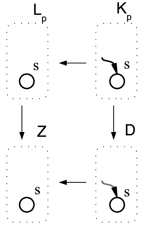
Moreover, in the case of general rules, the pushout complement in $\mathbf{ONet}$ might not be unique. In fact, whenever, as in Fig. 9, there is an open place in $K_{p}$ whose image is not open in $L_{p}$ (and thus neither in $Z$ ), then the corresponding place in $D$ can be either open or not. For instance, the diagram in Fig. 9 admits two possible pushout complements consisting of an open net $D$ with a single place $s$ which can be or not input open.

Under additional requirements it is possible to prove the existence of a minimal pushout complement $D$ , i.e., a pushout complement which embeds into any other and which is taken as a canonical choice. Roughly, the minimal pushout complement is the maximally open one: whenever a place could be either open or not, it is taken to be open (in Fig. 9, this corresponds to take the pushout complements $D$ with place $s$ input open).

Lemma 17 (existence of the pushout complement).

Let $p$ be a rewriting rule over open nets, let $Z$ be an open net and let $m:L_{p}\to Z$ be a match. Assume that

(1)

for all places $s\in L_{p}-l_{p}(K_{p})$ we have ${\rm Phys.~Rev.~E}[m(s)],{m(s)}{{}^{\bullet}}\subseteq m(L_{p}-l_{p}(K_{p}))$ ;
(2)

$m(l_{p}(\mathsf{in}({l_{p}}))\cap O_{L_{p}}^{+})\subseteq O_{Z}^{+}$ and $m(l_{p}(\mathsf{out}({l_{p}}))\cap O_{L_{p}}^{-})\subseteq O_{Z}^{-}$ ;
(3)

$m(O_{L_{p}}^{x}-l_{p}(O_{K_{p}}^{x}))\subseteq O_{Z}^{x}$ for $x\in\{+,-\}$ .

Then the pushout complement exists in $\mathbf{Net}$ , defined as $D=Z-m(L_{p}-l_{p}(K_{p}))$ , componentwise over the place and transition sets, and it can be lifted to a minimal pushout complement in $\mathbf{ONet}$ by taking as input open places:

$O_{D}^{+}=d^{-1}(O_{Z}^{+})\cup n(O_{K_{p}}^{+}-O_{L_{p}}^{+})$

Output open places are defined analogously. The initial marking $\hat{u}_{D}$ is defined by $\hat{u}_{D}(s)=\hat{u}_{Z}(d(s))$ for any place $s\in S_{D}$ .

Proof 6.2.

The proof is long, but straightforward. We have already motivated the dangling condition above. In order to understand condition 2, observe that, roughly, a place $s$ of $L_{p}$ is in $l_{p}(\mathsf{in}({l_{p}}))$ if applying the rule $p$ the place is preserved but at least one transition in ${\rm Phys.~Rev.~E}[s]$ is removed. Since the rule deletes an input transition from $m(s)$ – the image of $s$ in $Z$ – the corresponding place in $D$ belongs to $\mathsf{in}({d})$ and thus it must be input open. Therefore if $s$ is open also in $L_{p}$ , necessarily, by the construction of pushout in $\mathbf{ONet}$ , $m(s)$ must be open in $Z$ . Similarly, for condition 3, if a place is open in $L_{p}$ and it is not in the image of $K_{p}$ then necessarily it will be open in $Z$ .

Formally we have to show that (a) the mappings $n$ and $d$ are well-defined open net morphisms, (b) $l_{p}$ and $m$ are composable and (c) $Z$ is the pushout. Minimality of the pushout complement then follows by construction.

(a.1)
$n$ is a well-defined open net morphism.
Let us prove that $n^{-1}(O_{D}^{+})\cup\mathsf{in}({n})\subseteq O_{K}^{+}$ (the condition on output open places is analogous). If $s\in n^{-1}(O_{D}^{+})$ we have two possibilities according to the way $O_{D}^{+}$ is defined.
1. $-$
  
  If $n(s)\in d^{-1}(O_{Z}^{+})$ then $d(n(s))\in O_{Z}^{+}$ . Since $d\circ n=m\circ l_{p}$ and $m\circ l_{p}$ is a well-defined open net morphism, we deduce that $s\in O_{K}^{+}$ .
2. $-$
  
  If $n(s)\in n(O_{K}^{+}-O_{L}^{+})$ , since $n$ is injective, we have that $s\in O_{K}^{+}-O_{L}^{+}\subseteq O_{K}^{+}$ .
If instead $s\in\mathsf{in}({n})$ then $m(l_{p}(s))\in\mathsf{in}({m\circ l_{p}})$ . Since $m\circ l_{p}$ is an open net morphism, we conclude $s\in O_{K_{p}}^{+}$ , as desired.
Concerning the initial marking, note that for any $s\in S_{K}$ we have $\hat{u}_{K}(s)=\hat{u}_{Z}(m(l_{p}(s))=\hat{u}_{D}(d(n(s))=\hat{u}_{D}(s)$ , where the last equality holds by construction.
(a.2)
$d$ is a well-defined open net morphism.
Also in this case we only prove that $d^{-1}(O_{Z}^{+})\cup\mathsf{in}({d})\subseteq O_{D}^{+}$ (the condition on output open places is analogous). If $s\in d^{-1}(O_{Z}^{+})$ then $s\in O_{D}^{+}$ by definition. If, instead, $s\in\mathsf{in}({d})$ then it is easy to see that there exists $s^{\prime}\in S_{K}$ such that $s^{\prime}\in\mathsf{in}({l_{p}})\subseteq O_{K}^{+}$ . Now, there are two subcases:
1. $-$
  
  If $l_{p}(s^{\prime})\in O_{L}^{+}$ we have that $s^{\prime}\in l_{p}(\mathsf{in}({l_{p}}))\cap O_{L}^{+}$ and thus $m(s^{\prime})\in m(l_{p}(\mathsf{in}({l_{p}}))\cap O_{L}^{+})\subseteq O_{Z}^{+}$ by condition 2. Since $d(s)=m(s^{\prime})$ we deduce that $s\in d^{-1}(O_{Z}^{+})\subseteq O_{D}^{+}$ by construction of $D$ .
2. $-$
  
  If $l_{p}(s^{\prime})\not\in O_{L}^{+}$ then $s^{\prime}\in O_{K}^{+}-O_{L}^{+}$ , and thus $n(s^{\prime})\in n(O_{K}^{+}-O_{L}^{+})\subseteq O_{D}^{+}$ , by construction of $D$ .
The condition over the initial marking is trivially satisfied by construction.
(b)
$n$ and $l_{p}$ are composable.
We show the two conditions for composability separately:
1. $-$
  
  $n(\mathsf{in}({l_{p}}))\subseteq O_{D}^{+}$
  In fact, if $s\in\mathsf{in}({l_{p}})$ , then it is easy to see that $m(l_{p}(s))\in\mathsf{in}({d})\subseteq O_{D}^{+}$ . Now, $m(l_{p}(s))=d(n(s))$ and, since $d$ is an open net morphism, it must reflect open places, and thus $n(s)\in O_{D}^{+}$ .
2. $-$
  
  $l_{p}(\mathsf{in}({n}))\subseteq O_{L}^{+}$
  If $s\in l_{p}(\mathsf{in}({n}))$ then, it is easy to see that $s\in\mathsf{in}({m})\subseteq O_{L}^{+}$ , as desired.
(c)

$Z$ is the pushout.
We know that $Z$ is the pushout of $n$ and $l_{p}$ in $\mathbf{Net}$ . We have to prove that it is also a pushout in $\mathbf{ONet}$ .

Concerning the set of open places we have to show that

$O_{Z}^{x}\supseteq\{s\in S_{Z}:m^{-1}(s)\subseteq O_{L}^{x}\ \wedge\ d^{-1}(s)\subseteq O_{D}^{x}\}$ .

Then the converse inclusion, and thus equality, follows from the fact that $m$ and $d$ are open net morphisms.

Let $s\in S_{Z}$ such that there are $s^{\prime}\in O_{L}^{+}$ and $s^{\prime\prime}\in O_{D}^{+}$ such that $m(s^{\prime})=s=d(s^{\prime\prime})$ . Thus, there is $s^{\prime\prime\prime}\in S_{K}$ such that $l_{p}(s^{\prime\prime\prime})=s^{\prime}$ and $n(s^{\prime\prime\prime})=s^{\prime\prime}$ .

Since $s^{\prime\prime}\in O_{D}^{+}$ , then either $s^{\prime\prime}\in d^{-1}(O_{Z}^{+})$ or $s^{\prime\prime}\in n(O_{K}^{+}-O_{L}^{+})$ . Since $s^{\prime}\in O_{L}^{+}$ and $l_{p}(s^{\prime\prime\prime})=s^{\prime}$ , the second possibility cannot arise. In the first case $s=d(s^{\prime\prime})\in O_{Z}^{+}$ , as desired.

When $s$ is only in the image of $D$ , the proof is analogous. When it is only in the image of $L_{P}$ , we can use condition 3 in the hypothesis.∎

Summarizing, condition 1 of Lemma 17 is a dangling condition. By the remaining conditions, if a place $s$ in $L_{p}$ is open, and the rule prescribes either the deletion of incoming/outgoing transitions from such place (condition 2) or the deletion of the place itself (condition 3), then the image of $s$ in $Z$ must be open. Examples of what fails when conditions 2 and 3 are violated can be found in Fig. 9 and 9.

It is worth observing that in the case of rules $p$ such that morphism $l_{p}$ preserves open places, i.e., $l_{p}(O_{K_{p}}^{x})\subseteq O_{L_{p}}^{x}$ for $x\in\{+,-\}$ , the above result ensures the existence of a unique pushout complement.

Given a match $m:L_{p}\to Z$ as in the proposition above, the transformation can be completed if $n:K_{p}\to D$ and $r_{p}:K_{p}\to R_{p}$ are composable. For this we need to suitably restrict matches.

{defi}

[proper match] Let $p$ be a rewriting rule over open nets and let $Z$ be an open net. A match $m:L_{p}\to Z$ is called proper if it satisfies conditions 1, 2, and 3 in Lemma 17 and

(4)

for any $s\in K_{p}$ , if $s\in\mathsf{in}({r_{p}})-\mathsf{in}({l_{p}})$ then $m(l_{p}(s))\in O_{Z}^{+}$ ;
(5)

$r_{p}(l_{p}^{-1}(\mathsf{in}({m})))\subseteq O_{R_{p}}^{+}$ ;

plus the dual conditions on output places. Intuitively, a match is proper if whenever $s\in l_{p}(\mathsf{in}({r_{p}}))$ , i.e., the rule $p$ creates a new (ingoing) transition connected to place $s$ , then $m(s)$ is (input) open (condition 4). Additionally, input (output) places for the match which are preserved by the rule must be input (output) open in $R_{p}$ . An example in which condition 4 is violated can be found in Fig. 10. For place $s$ in $K_{p}$ we have $s\in\mathsf{in}({r_{p}})$ , since transition $t$ is added in $R_{p}$ , but $s\not\in\mathsf{in}({l_{p}})$ . Note that the mapping from $D$ to $Z^{\prime}$ is not a valid open net morphism, since place $s$ in $D$ is not open. In Fig. 10 instead is condition 5 which is violated. Place $s$ of $L_{p}$ is in $\mathsf{in}({m})$ , it is preserved by the rule, but the corresponding place in $R_{p}$ is not open. Again we cannot complete the DPO step since the mapping from $R_{p}$ to $Z^{\prime}$ is not a valid open net morphism (place $s$ should be input open in $R_{p}$ ).

We finally arrive at the desired result.

Lemma 18 (applying general rules).

Let $p$ be a rule over open nets, let $Z$ be an open net and let $m:L_{p}\to Z$ be a proper match. Then there exists a transformation $Z\Rightarrow^{p,m}Z^{\prime}$ .

Proof 6.3.

Let $p$ be a rule over open nets, let $Z$ be an open net and let $m:L_{p}\to Z$ be a proper match. Then, by using Lemma 17 we can construct the minimal pushout complement of $l_{p}$ and $m$ , as in Fig. 8(a).

In order to conclude, it suffices to show that $n$ and $r_{p}$ are composable. To this aim observe that by properness of the match:

$\bullet$

$n(\mathsf{in}({r_{p}}))\subseteq O_{D}^{+}$ (and the same condition holds for $\mathsf{out}({.})$ )
In fact, let $s\in\mathsf{in}({r_{p}})$ We distinguish two possibilities. If $s\in\mathsf{in}({l_{p}})$ then necessarily $n(s)\in\mathsf{in}({d})$ and thus $n(s)\in O_{D}^{+}$ , since $n$ is an open net morphism. If instead, $s\not\in\mathsf{in}({l_{p}})$ , then $s\in\mathsf{in}({r_{p}})-\mathsf{in}({l_{p}})$ , hence, by condition 4 of Definition 6.2, $m(l_{p}(s))\in O_{Z}^{+}$ . Since $m(l_{p}(s))=d(n(s))$ and $d$ is an open net morphism, we conclude that also in this case $n(s)\in O_{D}^{+}$ .
$\bullet$

$r_{p}(\mathsf{in}({n}))=r_{p}(l_{p}^{-1}(\mathsf{in}({m})))\subseteq O_{R_{p}}^{+}$ (and the same condition holds for $\mathsf{out}({.})$ )
Immediate by condition 5 of Definition 6.2.∎

6.2.2. Applying Behaviour Preserving Rules.

Sufficient hypotheses which ensure the applicability of behaviour preserving rules are made explicit in the following statement. This is a corollary of the general theory of transformations for open nets developed before.

Corollary 19 (applying behaviour preserving rules).

Let $p$ be a $\mathsf{x}$ -behaviour preserving rule, let $Z$ be an open net and let $m:L_{p}\to Z$ be a match such that:

a.

for all $s\in L_{p}-l_{p}(K_{p})$ we have ${\rm Phys.~Rev.~E}[m(s)]\cup{m(s)}{{}^{\bullet}}\subseteq m(L_{p}-K_{p})$ ;
b.

for all $s\in K_{p}$ , if $s\in\mathsf{in}({l_{p}})$ and $l_{p}(s)\in O_{L_{p}}^{+}$ then $m(l_{p}(s))\in O_{Z}^{+}$ ;
c.

for all $s\in K_{p}$ , if $s\in\mathsf{in}({r_{p}})-\mathsf{in}({l_{p}})$ then $m(l_{p}(s))\in O_{Z}^{+}$ ;

and the dual of the last two conditions, obtained by replacing $\mathsf{in}({})$ by $\mathsf{out}({})$ and $+$ by $-$ , hold. Then, there exists a transformation $Z\Rightarrow^{p,m}Z^{\prime}$ .

Proof 6.4.

This is an easy consequence of Lemma 18. We need to show that conditions (a)-(c) ensure that the match $m$ is proper, i.e., it satisfies conditions 1–5 of Lemma 17 and Definition 6.2.

Condition 1 is the same as condition (a), condition 2 is just a compact notation for condition (b) and condition 4 is exactly condition (c). Concerning condition 3, observe that, since $p$ is a behaviour preserving rule then $(r_{p}\circ l_{p}^{-1})_{|O_{L_{p}}}$ is a correspondence between the left- and right-hand side. This means that for any place $s$ in $O_{L_{p}}^{x}$ there must be a place $s^{\prime}$ in $K_{p}$ such that $l_{p}(s^{\prime})=s$ , and, by definition of open net morphism $s^{\prime}$ must be open, i.e., $s^{\prime}\in O_{K_{p}}^{x}$ . Therefore $O_{L_{p}}^{x}\subseteq l_{p}(O_{K_{p}}^{x})$ and thus condition 3 is trivially satisfied. Similarly, for condition 5, observe that, by definition of open net morphisms, $\mathsf{in}({m})\subseteq O_{L_{p}}^{+}$ , and, thus

$r_{p}(l_{p}^{-1}(\mathsf{in}({m})))\subseteq r_{p}(l_{p}^{-1}(O_{L_{p}}^{+}))=O_{R_{P}}^{+}$ .

The last equality is justified by the fact that $p$ is behaviour preserving, and thus, as observed above, $(r_{p}\circ l_{p}^{-1})_{|O_{L_{p}}}$ is a correspondence between $L_{p}$ and $R_{p}$ .

The intuition underlying the conditions above is the following. Condition (a) is a typical dangling condition, which we have already commented. Condition (b) says that if $s\in\mathsf{in}({l_{p}})$ , i.e., if some (ingoing) transitions are deleted from $s$ then the image of $s$ in $Z$ must be (input) open if so is its image in $L_{p}$ . Finally, by condition (c), if $s\in\mathsf{in}({r_{p}})-\mathsf{in}({l_{p}})$ , i.e., the rule $p$ creates a new (ingoing) transition connected to place $s$ , without replacing any old one, then the image of $s$ in $Z$ must be (input) open.

As an example, consider again the DPO diagram in Fig. 8(b). It is not difficult to see that the rule and the match satisfy the conditions of Corollary 19. Hence we can complete the double-pushout construction transforming $Z$ into $Z^{\prime}$ , as depicted in the same figure.

6.3. Modeling Dynamic Reconfigurations of Services

Open nets allow us to specify a system as built out of smaller components. Then, its behaviour is captured by the firing or step behaviour of the open net. However, for highly dynamic systems, as mentioned in the introduction, it can be useful to have the possibility of specifying that, under suitable conditions, some structural changes or reconfigurations of the system can take place. For instance the invocation of a service could trigger a rule which provides an implementation of the required service.

The theory of open net reconfigurations can do the job. As an example, consider net $Z_{0}$ in Fig. 12 which models the view of a traveller on the journey planning and ticket purchase services offered through a travel agency portal.

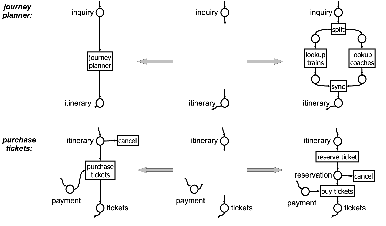
We distinguish abstract transitions representing services that should be provided elsewhere and concrete transitions representing local services and control flow actions. The invocation of an external service can be seen at different levels of abstraction. From the point of view of the client process it is just the firing of an abstract transition. At a lower level of abstraction, it is captured by a rule such as the one at the top of Fig. 11. An application of this rule, replacing the abstract transition by a new open net, models the discovery and binding of the concrete services required. The left- and right-hand sides of the rule are weakly firing (actually, also step) bisimilar if we observe only the interactions at the open (interface) places, i.e., if we take $\Lambda_{\tau}=\Lambda$ . This can be seen as a proof of the fact that the bound service meets the requirements: both in the abstract transition and in its concrete counterpart any inquiry will produce a corresponding itinerary.

The rule at the bottom of Fig. 11 represents a case where a simple pattern is replaced by a richer one. On the left we say that, given an itinerary, we can either purchase the required tickets or cancel the processes. On the right the transaction is refined, adding a prior reservation phase, while keeping the option to cancel. As above, the rule has weakly firing (and step) bisimilar left- and right-hand sides, ensuring that the visible effect of the abstract and concrete transitions at the interfaces is the same.

A possible sequence of transformations is shown in Fig. 12. By Theorem 16, we are sure that the transformations do not change the observable behaviour of the system, i.e., the start and end nets are weakly bisimilar, a fact that can be interpreted as a proof of conformance of the provided service with respect to the abstract specification.

We have shown only a small example application, however, we believe that this technique can be applied to larger case studies, such as the banking scenario studied in [12]. In order to do this automatically, it would be necessary to implement mechanized bisimulation checking procedures. For finite state spaces, this is quite straightforward, for infinite state spaces we could resort to the techniques presented in [15]. In any case the up-to technique presented in Section 5 will be very useful for practical case studies.

Another relevant question is the following: which kind of bisimilarity should be used? While strong firing bisimilarity is conceptually the simplest behavioural equivalence, practical examples usually require weak bisimulations in order to abstract from internal or silent moves. Finally, step bisimulation is able to distinguish processes that differ with respect to the degree of concurrency. This can be relevant if the observer is able to distinguish different degrees of parallelism or if we take into account efficiency questions.

7. Conclusions and Related Work

Open nets, introduced in [3, 4], are a reactive extension of standard Petri nets which allows to model systems interacting with an unspecified environment.

As mentioned in the introduction there is a vast related literature. A close conceptual relationship exists with the early studies on modular construction and refinement techniques (see, e.g., [37, 36, 28, 41]) and on composition operators and compositional semantics for Petri nets (see, e.g., [1, 9, 6, 46]). The last class comprises also the algebraic approaches to Petri nets which view the class of Petri nets as a category and, characterising the semantics of interest as a universal constructions, automatically deduce the compositionality for suitably defined operators [47, 48, 24].

More recent approaches, which focus more explicitly on the definition of notion of module and interface and where the reactive aspects are taken into account in the semantics can be classified roughly into two classes. Some approaches aim at defining a “calculus of nets”, where a set of process algebra-like operators allow one to build complex nets starting from a set of predefined basic components. In this family, the papers [29, 33] propose an algebra of (labelled) Petri nets with interfaces, consisting of public (input) places and (output) transitions, with operators which allow e.g., to add new transitions and places, to connect existing public transitions and places by new arcs, to hide items in the net. We also recall the Petri Box calculus [10, 18, 17], where a special class of safe nets, called plain boxes, provides the basic components, which are then combined by means of (refinement-based) composition operators. Another family of approaches can be classified as “component-oriented”: the emphasis, rather than on the algebraic aspects, is put on the mechanisms which allow one to build larger systems by combining nets with clearly identified interfaces. For instance the book [43] proposes a technique for inserting a net, called daughter net, into a so-called host net. The composition is realised by joining the two nets along a predefined set of places, playing the role of open places. The distinction between input and output open places, absent in [43], instead is later considered in [45]. A compositionality result is proved for language equivalence and a notion of bisimilarity, very close to ours, is defined. Interestingly, the same book also focuses on an alternative approach to net composition, based on an operation of synchronised parallel product in the style of [48]. Such operation, roughly speaking, joins two nets by forcing the synchronisation of transitions with the same label. Other members of the “component-oriented” family are, for example, the Petri net components [16] and the nets with pins [5]. We also recall workflow nets [38] which have been proposed as a formal model for the description of workflows, i.e., business processes specified in terms of tasks and shared resources. Workflow nets are special Petri nets satisfying suitable conditions, like the existence of one initial and one final place: tokens in such places characterise the start and the end, respectively, of the represented process. The model has been extended for the specification of interorganisational workflows [39], represented as a set of workflow nets connected through additional places for asynchronous communication and synchronisation requirements on transitions. Additional references, as well as a detailed comparison between the approaches to Petri net composition and reactivity just cited and the open net model can be found in [4].

In this paper, firstly we have generalised the theory of open nets, including the characterisation of net composition using pushouts, to the case of marked nets. Next we have introduced several natural notions of bisimilarity over open nets, showing that weak bisimilarities, arising in the presence of unobservable actions, and, as a particular case, also strong bisimilarities are congruences with respect to the colimit-based composition operation over open nets. The considered notions of bisimilarity differ for the choice of the observations. These can be single firings, thus leading to what we called firing bisimilarity, a standard notion of interleaving equivalence, capable of capturing the branching structure of computations. Alternatively, we can observe parallel steps, thus obtaining step bisimilarity, which allows to capture, to some extent, the degree of parallelism that is possible in a component. This can be useful, e.g., when a component is replaced by another one since we might be interested in taking a replacement that exhibits at least the same concurrent behaviour and is hence equally efficient.

In recent years, reactive extensions of Petri nets have been obtained by exploiting a general theory of reactive systems developed for automatically deriving bisimulation congruences. Specifically, an encoding of Petri nets as bigraphical reactive systems has been proposed in [27], while [35] proposes an encoding of nets as reactive systems in the cospan category over an adhesive category. Our results about strong firing bisimilarity can be seen as a generalisation of those in [27, 35], which essentially are developed for a special kind of open nets, where there is no distinction between input and output open places. Furthermore the composition operation used in the cited papers does not allow synchronisation of transitions (technically, the interface net does not contain transitions).

Concerning weak step bisimilarity, some connections seem to exist with the work on action refinement, which goes back to [37]. For example, in [44] (weak) step bisimilarity is shown to be a congruence with respect to a refinement operation which allows to replace a single event with a deterministic finite event structure. Although the setting is different and a direct comparison is not possible, we observe that, compared to refinement-based approaches, where single transitions are refined by a subnet, the theory presented here works for general reconfigurations, in which both the left- and right-hand sides can be general, arbitrarily large nets.

Weak (step) bisimilarity for Petri nets is studied also in [29]. They observe that such an equivalence is not a congruence in general, but for Petri nets satisfying a suitable condition on the labelling of the public transitions (well-labelled nets), a context closure allows one to get a congruence which is then characterised by means of a universal context. The setting is different from ours since the issue of net composition is tackled at a finer level of granularity: the basic components of a net are assumed to be transitions with empty pre- and post-set and single places, which are then combined by means of constructors that allow one to connect places and transitions. Still it would be interesting to understand if a formal relation can be established, e.g., trying to internalise the pushout-based composition operation in the algebra of connectors of [29].

Similarities exist also with the problem studied in [11], where a reactive Petri net model which admits a compositional behavioural equivalence is exploited, in the framework of web-services, to provide a theoretical basis to service composition and discovery. This technique is then used in a case study for checking the correctness of service specifications and the replaceability of services in a banking scenario [12]. Disregarding the technical differences, such as the fact that the mentioned paper deals with C/E nets and the use of read arcs, the kind of nets of interest for this approach are essentially a subclass of open Petri nets, satisfying some structural requirements (all labels are invisible and the interface consists of a single input and a single output place, plus some read places). Generally speaking, compositional Petri net models appears to be promising as a formalism for the specification of control and composition in service oriented architectures as suggested, e.g., in [8, 22, 40, 23]. Investigating possible applications of (reconfigurable) open Petri nets, along the lines of the presented example, in the setting of web-service specification and analysis represent a stimulating direction of future research.

In the second part of the paper we have proposed a rewriting-based framework for Petri nets with reconfigurations. We have shown how our congruence results can be used to identify classes of reconfigurations which do not alter the observational behaviour of the system. This is applied to a small case study of a workflow-like model of a travel agency, where we showed how abstract services can be replaced by more concrete implementations and how we can ensure that the behaviour of the full net is preserved under such operations.

Action refinement of Petri nets (see, e.g., [37, 36, 28, 41]), that we already mentioned above, can be seen as a special form of reconfiguration. The idea of using rewriting techniques for providing a reconfiguration mechanism for Petri nets has been already explored in the literature (see, e.g., reconfigurable nets of [2, 21] and high-level replacement systems applied to Petri nets in [31]). In this approaches, however, the emphasis is more on rewriting as a computational mechanism, rather than on the study of the way the behaviour of the system is affected by the reconfigurations. In future work, besides deepening the relationships between these approaches and ours, we will continue studying the notion of reconfigurable open nets and describe in more detail how reconfigurations can be triggered by the net itself, for example by reaching certain markings or by firing certain transitions, following an intuition similar to that of dynamic nets [13].

Finally, it would be worth studying whether a formal duality can be established between our morphisms and standard simulation morphisms for Petri nets. Viewing our morphisms as inverses of (partial) simulation morphisms would allow to get a precise correspondence between our pushout-based composition and pullback-based synchronisation of Petri nets. Surely by simply taking Winskel’s morphisms [47] this does not work (technically because when they are undefined on a transition they must be undefined on the corresponding pre- and post-set). Also more general morphisms for Petri nets, like those proposed in [42, 7], would not provide an immediate solution. Still, it looks feasible to identify generalisations of such morphisms to the context of open Petri nets allowing to develop a dual theory based on simulations.

Acknowledgement: We would like to thank the referees for their insightful and detailed comments.

References

[1] C. André. The behaviour of a Petri net on a subset of transitions. RAIRO, 17:5–21, 1983.
[2] E. Badouel, M. Llorens, and J. Oliver. Modeling concurrent systems: Reconfigurable nets. In H. R. Arabnia and Y. Mun, editors, Proceedings of PDPTA’03, volume 4, pages 1568–1574. CSREA Press, 2003.
[3] P. Baldan, A. Corradini, H. Ehrig, and R. Heckel. Compositional modeling of reactive systems using open nets. In K.G. Larsen and M. Nielsen, editors, Proceedings of CONCUR’01, volume 2154 of LNCS, pages 502–518. Springer Verlag, 2001.
[4] P. Baldan, A. Corradini, H. Ehrig, and R. Heckel. Compositional semantics for open Petri nets based on deterministic processes. MSCS, 15(1):1–35, 2005.
[5] T. Basten. In terms of nets: System design with Petri nets and process algebra. PhD thesis, Eindhoven University of Technology, 1998.
[6] B. Baumgarten. On internal and external characterisation of PT-net building block behaviour. In G. Rozenberg, editor, Advances in Petri nets, volume 340 of LNCS, pages 44–61. Springer, 1988.
[7] M. A. Bednarczyk and A. M. Borzyszkowski. General morphisms of Petri nets (extended abstract). In J. Wiedermann, P. van Emde Boas, and M. Nielsen, editors, Proceedings of ICALP’99, volume 1644, pages 190–199. Springer Verlag, 1999.
[8] B. Benatallah and R. Hamadi. A Petri net-based model for Web service composition. In K.-D. Schewe and X. Zhou, editors, Australasian Database Conference, Conferences in Research and Practice in Information Technology, volume 7, pages 191–200. Australian Computer Society, 2003.
[9] G. Berthelot. Transformations and decompositions of nets. In W. Brauer, editor, Petri Nets: Central models and their properties, volume 254 of LNCS, pages 359–376. Springer, 1987.
[10] E. Best, R. Devillers, and J. G. Hall. The Petri box calculus: a new causal algebra with multi-label communication. In G. Rozenberg, editor, Advances in Petri Nets, volume 609 of LNCS, pages 21–69. Springer Verlag, 1992.
[11] F. Bonchi, A. Brogi, S. Corfini, and F. Gadducci. A behavioural congruence for web services. In Proceedings of FSEN ’07, volume 4727 of LNCS, pages 240–256. Springer, 2007.
[12] F. Bonchi, A. Brogi, S. Corfini, and F. Gadducci. Compositional specification of web services via behavioural equivalence of nets: A case study. In Proc. of Petri Nets ’08, pages 52–71, 2008.
[13] M.G. Buscemi and V. Sassone. High-level Petri nets as type theories in the join calculus. In Proceedings of FoSSaCS’01, volume 2030 of LNCS, pages 104–120. Springer, 2001.
[14] H. Ehrig. Tutorial introduction to the algebraic approach of graph-grammars. In H. Ehrig, M. Nagl, G. Rozenberg, and A. Rosenfeld, editors, Proceedings of the 3rd International Workshop on Graph-Grammars and Their Application to Computer Science, volume 291 of LNCS, pages 3–14. Springer Verlag, 1987.
[15] D. Hirschkoff. Automatically proving up to bisimulation. In Proc. of MFCS ’98 Workshop on Concurrency, number 18 in ENTCS, 1998.
[16] E. Kindler. A compositional partial order semantics for Petri net components. In P. Azema and G. Balbo, editors, Application and Theory of Petri Nets, volume 1248 of LNCS, pages 235–252. Springer Verlag, 1997.
[17] M. Koutny and E. Best. Operational and denotational semantics for the box algebra. Theoretical Computer Science, 211(1–2):1–83, 1999.
[18] M. Koutny, J. Esparza, and E. Best. Operational semantics for the Petri box calculus. In B. Jonsson and J. Parrow, editors, Proceedings of CONCUR ’94, volume 836 of LNCS, pages 210–225. Springer Verlag, 1994.
[19] S. Lack and P. Sobociński. Adhesive and quasiadhesive categories. RAIRO – Theoretical Informatics and Applications, 39(3):511–555, 2005.
[20] J. Leifer and R. Milner. Deriving bisimulation congruences for reactive systems. In C. Palamidessi, editor, Proceedings of CONCUR’00, volume 1877 of LNCS, pages 243–258. Springer Verlag, 2000.
[21] M. Llorens and J. Oliver. Introducing structural dynamic changes in Petri nets: Marked-controlled reconfigurable nets. In F. Wang, editor, Proceedings of ATVA’04, volume 3299, pages 310–323. Springer Verlag, 2004.
[22] A. Martens. Analyzing Web service based business processes. In M. Cerioli, editor, Proceedings of FASE’05, volume 3442 of LNCS, pages 19–33. Springer, 2005.
[23] P. Massuthe, W. Reisig, and K. Schmidt. An Operating Guideline Approach to the SOA. Annals of Mathematics, Computing & Teleinformatics, 1(3):35–43, 2005.
[24] J. Meseguer and U. Montanari. Petri nets are monoids. Information and Computation, 88:105–155, 1990.
[25] R. Milner. A Calculus of Communicating Systems, volume 92 of LNCS. Springer Verlag, 1980.
[26] R. Milner. Bigraphical reactive systems. In K. G. Larsen and M. Nielsen, editors, Proceedings of CONCUR’01, volume 2154 of LNCS, pages 16–35. Springer Verlag, 2001.
[27] R. Milner. Bigraphs for Petri nets. In J. Desel, W. Reisig, and G. Rozenberg, editors, Lectures on Concurrency and Petri Nets, volume 3098 of LNCS, pages 686–701. Springer, 2003.
[28] K. Müller. Constructable Petri nets. Elektr. Inf. Kybern., 21:171–199, 1985.
[29] M. Nielsen, L. Priese, and V. Sassone. Characterizing Behavioural Congruences for Petri Nets. In Proceedings of CONCUR’95, volume 962 of LNCS, pages 175–189. Springer Verlag, 1995.
[30] M. Nielsen and P. S. Thiagarajan. Degrees of non-determinism and concurrency: A Petri net view. In M. Joseph and R. Shyamasunda, editors, Proceedings of FSTTCS’84, pages 89–117. Springer Verlag, 1984.
[31] J. Padberg, H. Ehrig, and L. Ribeiro. High level replacement systems applied to algebraic high level net transformation systems. Mathematical Structures in Computer Science, 5(2):217–256, 1995.
[32] B. Pierce. Basic Category Theory for Computer Scientists (Foundations of Computing). MIT Press, 1991.
[33] L. Priese and H. Wimmel. A uniform approach to true-concurrency and interleaving semantics for Petri nets. Theoretical Computer Science, 206(1–2):219–256, 1998.
[34] W. Reisig. Petri Nets: An Introduction. EATCS Monographs on Theoretical Computer Science. Springer Verlag, 1985.
[35] V. Sassone and P. Sobocinski. A congruence for Petri nets. In Proceedings of PNGT’04, volume 127(2) of Electronic Notes in Theoretical Computer Science, pages 107–120. Elsevier Science, 2005.
[36] I. Suzuki and T. Murata. A method for stepwise refinement and abstraction of Petri nets. Journal of computer and system sciences, 27:51–76, 1983.
[37] R. Valette. Analysis of Petri nets by stepwise refinements. Journal of Computer and System Sciences, 18(1):35–46, 1979.
[38] W. van der Aalst. The application of Petri nets to workflow management. The Journal of Circuits, Systems and Computers, 8(1):21–66, 1998.
[39] W. van der Aalst. Interorganizational workflows: An approach based on message sequence charts and Petri nets. System Analysis and Modeling, 34(3):335–367, 1999.
[40] W.M.P. van der Aalst and A.H.M. ter Hofstede. Yawl: yet another workflow language. Information Systems, 30(4):245–275, 2005.
[41] W. Vogler. Behaviour preserving refinement of Petri nets. In G. Tinhofer and G. Schmidt, editors, Proceedings of WG’86: Graph theoretic concepts in computer sciencea, volume 246 of LNCS, pages 82–93. Springer, 1987.
[42] W. Vogler. Executions: A new partial-order semantics of Petri nets. Theoretical Computer Science, 91(2):205–238, 1991.
[43] W. Vogler. Modular Construction and Partial Order Semantics of Petri Nets, volume 625 of LNCS. Springer, 1992.
[44] W. Vogler. Bisimulation and action refinement. Theoretical Computer Science, 114(1):173–200, 1993.
[45] W. Vogler. Efficiency of asynchronous systems that communicate asynchronously. In Proc. of ICATPN ’00, volume 1825 of LNCS, pages 424–444, 2000.
[46] K. Voss. Interface as a basic concept for system specification. In K. Voss, editor, Concurrency and Nets, pages 585–604. Springer, 1987.
[47] G. Winskel. Event Structures. In Petri Nets: Applications and Relationships to Other Models of Concurrency, volume 255 of LNCS, pages 325–392. Springer Verlag, 1987.
[48] G. Winskel. Petri nets, algebras, morphisms, and compositionality. Information and Computation, 72(3):197–238, 1987.

$u_{1}^{I}\ [\/{A_{1}^{I}}\/\rangle\ v_{1}^{I}$	$u_{2}^{E}\ [\/{A_{2}^{E}}\/\rangle\ v_{2}^{E}$ ,	$({u_{1}^{I}}\!\downarrow\!{f_{1}})=({u_{2}^{E}}\!\downarrow\!{f_{2}})$
$u_{1}^{E}\ [\/{A_{1}^{E}}\/\rangle\ v_{1}^{E}$ ,	$u_{2}^{I}\ [\/{A_{2}^{I}}\/\rangle\ v_{2}^{I}$ ,	$({u_{1}^{E}}\!\downarrow\!{f_{1}})=({u_{2}^{I}}\!\downarrow\!{f_{2}})$

$A_{1}^{I}=({A_{3}^{1}}\!\Downarrow\!{\alpha_{1}})$		$A_{1}^{E}=A_{1}\ominus A_{1}^{I}$
$A_{2}^{I}=({(A_{3}^{2}\oplus A_{3}^{0}\oplus A_{3}^{open})}\!\Downarrow\!{\alpha_{2}})$		$A_{2}^{E}=A_{2}\ominus A_{2}^{I}$

${\rm Phys.~Rev.~E}[A_{1}]={f}_{1}^{\oplus}(({{\rm Phys.~Rev.~E}[A_{2}]}\!\downarrow\!{f_{2}}))$
$\leq{f}_{1}^{\oplus}(({u_{2}}\!\downarrow\!{f_{2}}))$
$={f}_{1}^{\oplus}(({u_{1}}\!\downarrow\!{f_{1}}))$		[since $({u_{2}}\!\downarrow\!{f_{2}})=({u_{1}}\!\downarrow\!{f_{1}})$ ]
$\leq u_{1}$		[by Lemma 2.(4)]

$B_{2}^{E}=A_{2}^{E}$		[by (7)]
$={f}_{2}^{\oplus}(({A_{1}^{I}}\!\Downarrow\!{f_{1}}))=$		[by (4)]
$={f}_{2}^{\oplus}(({B_{1}^{I}}\!\Downarrow\!{f_{1}}))=$		[by (14)]
$={g_{2}}^{\oplus}(({B_{1}^{I}}\!\Downarrow\!{f_{1}}))=$		[since $g_{2}$ and $f_{2}$ “agree” on $O_{Z_{0}}$ ]

Abstract.

Key words and phrases:

1991 Mathematics Subject Classification

Introduction

1. Marked Open Nets

Proposition 1.

Proof 1.1.

Lemma 2 (properties of projection).

Proof 1.2.

Lemma 3 (reflection of behaviour).

Proof 1.3.

2. Composing Open Nets

Proposition 4 (composition of multisets).

Proof 2.1.

Proposition 5 (pushouts in 𝐎𝐍𝐞𝐭\mathbf{ONet}).

Proof 2.2.

3. Composing Steps

Lemma 6.

Proof 3.1.

Lemma 7 (composing steps).

Proof 3.2.

4. Bisimilarity of Open Nets

4.1. A High Level View on the Congruence Results

Theorem 8 (bisimilarity is a congruence).

4.2. Proofs of the Congruence Results

Lemma 9.

Proof 4.1.

4.2.1. Strong Step Bisimilarity

Theorem 10.

Proof 4.2.

4.2.2. Weak Step Bisimilarity

Theorem 11.

Proof 4.3.

4.2.3. Weak (and Strong) Firing Bisimilarity

Theorem 12.

Proof 4.4.

4.3. Comparison to CCS

5. Some Proof Techniques for Bisimilarity

Proposition 13 (“closing” open places).

Proof 5.1.

Lemma 14.

Proof 5.2.

Proposition 15.

Proof 5.3.

6. Reconfigurations of Open Nets

6.1. Behaviour Preserving Reconfigurations of Open Nets

Theorem 16 (behaviour-preserving reconfigurations).

Proof 6.1.

6.2. Applying Rules to Open Nets

6.2.1. Applying General Rules.

Lemma 17 (existence of the pushout complement).

Proof 6.2.

Lemma 18 (applying general rules).

Proof 6.3.

6.2.2. Applying Behaviour Preserving Rules.

Corollary 19 (applying behaviour preserving rules).

Proof 6.4.

6.3. Modeling Dynamic Reconfigurations of Services

7. Conclusions and Related Work

References

Proposition 5 (pushouts in $\mathbf{ONet}$ ).