跳到论文正文
W Papers独立论文阅读器 arXiv:0809.4076 论文正文 计算阅读时间 · 0%
引用这篇论文根据当前论文元数据生成,正式投稿前建议核对。


License: arXiv.org perpetual non-exclusive license
arXiv:0809.4076v3 [gr-qc] 05 Jan 2009

Thick de Sitter brane solutions in higher dimensions

Preprint: CQUeST-2009-0240
Vladimir Dzhunushaliev Note: Senior Associate of the Abdus Salam ICTP Affiliation: Arnold-Sommerfeld-Center for Theoretical Physics, Department für Physik, Ludwig-Maximilians-Universität, Theresienstr. 37, D-80333, Munich, Germany
and
Department of Physics and Microelectronic Engineering, Kyrgyz-Russian Slavic University, Bishkek, Kievskaya Str. 44, 720021, Kyrgyz Republic
Email: vdzhunus@krsu.edu.kg
   Vladimir Folomeev Affiliation: Institute of Physics of National Academy of Science Kyrgyz Republic, 265 a, Chui Street, Bishkek, 720071, Kyrgyz Republi Email: vfolomeev@mail.ru    Masato Minamitsuji Email: minamituzi”at”sogang.ac.kr Affiliation: Arnold-Sommerfeld-Center for Theoretical Physics, Department für Physik, Ludwig-Maximilians-Universität, Theresienstr. 37, D-80333, Munich, Germany
and
Center for Quantum Spacetime, Sogang University, Shinsu-dong 1, Mapo-gu, 121-742 Seoul, South Korea
Abstract

We present thick de Sitter brane solutions which are supported by two interacting phantom scalar fields in five-, six- and seven-dimensional spacetime. It is shown that for all cases regular solutions with anti-de Sitter asymptotic (5D problem) and a flat asymptotic far from the brane (6D and 7D cases) exist. We also discuss the stability of our solutions.

Keywords: 
Higher-dimensional gravity, Cosmology
pacs
04.50.+h, 98.80.Cq

I introduction

In recent years, there is growing interest in higher-dimensional cosmological models inspired by the recent developments in string theory. One sort of such models are branes which are submanifolds embedded into the higher-dimensional spacetime. They play an important (even essential) role, for instance, in a description of the confinement of the nongravitational interactions and/or stabilization of the extra dimensions. Braneworld models, in which our universe is exactly one of four-dimensional branes, are the central issues in this research field. Much efforts to reveal cosmology on the brane have been done in the context of five-dimensional spacetime, especially after the stimulating proposals by Randall and Sundrum [1] (see, e.g., [2]). But of course there is no particular reason to restrict the number of dimensions to be five. In recent years, the focus has turned to higher-dimensional braneworld models.

It is still unclear how the gravity and cosmology on the brane embedded in the higher-dimensional spacetime behave. In higher dimensions, there would be many kinds of classes of possible braneworld models. Here we focus on the generic feature of higher-dimensional braneworld models and from this we deduce the subject to be revealed in this paper.

It is commonly assumed that a brane is an infinitely thin object. In five dimensions, this is a good approximation as long as one is interested in the scales larger than the brane thickness. Then, the cosmology on the brane in five dimensions, i.e., dynamics of the brane in one bulk spacetime, is uniquely determined by the Israel junction conditions once the matter on the brane is specified. But, in higher dimensions the situation is quite different. It happens because self-gravity of an infinitesimally thin three-brane in a higher-dimensional spacetime develops a severe singularity and one cannot put any kind of matter on the brane if the number of codimensions is larger than 2. Also in the case of a codimension-two brane, one cannot put any kind of matter other than the pure tension. The cosmology on such a brane must be investigated under some prescription of the singular structure of the brane. The well-motivated prescription is to regularize the brane by taking its microscopic structure into consideration. However, in the case of six-dimensional models, the cosmology on the brane strongly depends on the way of regularization. This implies that there is no unique brane cosmology in the case of higher codimensions.

Thus, in this paper we take a different point of view. We shall take the brane thickness into account from the beginning and look for the regular braneworld solutions with finite thickness, called thick brane solutions, in a field theory model. The thickness of the brane may be very close to the length scale of the quantum gravitational theory, e.g., the string length scale. As we mentioned, the brane thickness must be more essential in higher-dimensional spacetimes than in the five-dimensional one. Thus, we look for the thick brane solutions in higher dimensions as well as in five dimensions. Bearing the cosmological applications, we focus on the thick brane solutions which have de Sitter geometry in the ordinary four-dimensions.

The properties of thick branes in five-dimensions, especially localization of gravity, have been discussed in Ref. [3]. In five dimensions, the thick brane solutions in five-dimensional spacetime have been explored in various literatures (see, e.g., [4]). In this paper, we consider thick brane solutions supported by two interacting scalar fields ϕ\phi and χ\chi, whose potential is given by

V⁡(ϕ,χ)=λ14​(ϕ2−m12)2+λ24​(χ2−m22)2+λ3​ϕ2​χ2+Λ.V(\phi,\chi)=\frac{\lambda_{1}}{4}(\phi^{2}-m_{1}^{2})^{2}+\frac{\lambda_{2}}{4}(\chi^{2}-m_{2}^{2})^{2}+\lambda_{3}\phi^{2}\chi^{2}+\Lambda. (1)

A stronger interaction between two scalar fields develops the local metastable vacua, which may be able to support our brane universe, other than the global one. Several works on thick brane solutions in such a setup have already been performed. Five-dimensional Minkowski brane solutions were derived in [5, 6]. Bearing cosmological applications in mind, our goal in this work is to find thick de Sitter brane solutions. Thick brane solutions in higher-dimensional spacetimes with two interacting scalar field were also investigated in [7] (see, e.g., [8] for other kinds of models). We shall give de Sitter versions of these solutions.

In Ref. [9] there are some arguments in favor of the fact that the scalar fields, used in [7], are a quantum nonperturbative condensate of a SU(3) gauge field. Briefly these arguments consist of the following: components of the SU(3) gauge field can be divided in some natural way onto two parts. The first group contains those components which belong to a subgroup S​U​(2)∈S​U​(3)SU(2)\in SU(3). The remaining components belong to a factor space S​U​(3)/S​U​(2)SU(3)/SU(2). Following Heisenberg’s idea [10] about the non-perturbative quantization of a nonlinear spinor field the nonperturbative quantization for the SU(3) gauge field is being carried out as followings. It is supposed that two-point Green functions can be expressed via the scalar fields. The first field ϕ\phi describes two-point Green functions for SU(2) components of a gauge potential, and the second scalar field χ\chi describes two-point Green functions for S​U​(3)/S​U​(2)SU(3)/SU(2) components of the gauge potential. It is supposed further that four-point Green functions can be obtained as some bilinear combination of the two-point Green functions. Consequently, the Lagrangian of the SU(3) gauge field takes the form (2). It allows us to regard such sort of thick brane solutions as some defect in a spacetime filled by a condensate of the gauge field living in the bulk.

This paper is organized as follows. In Sec. II, we introduce the basic field theory model to find thick brane solutions. In Sec. III, we present thick brane solutions in five-, six- and seven-dimensional models. In Sec. IV, we investigate perturbations in the five-dimensional model and then give speculations about stability of higher-dimensional models. Secion V contains a brief summary.

II Basic theory

Our interest is in the D=(4+n)D=(4+n)-dimensional Einstein-scalar theory whose action is given by

S=∫dD​x​−g​{−Mn+4n+22​R+ϵ⁡[12​∂Aϕ​∂Aϕ+12​∂Aχ​∂Aχ−V⁡(ϕ,χ)]},S=\int d^{D}x\sqrt{-g}\left\{-\frac{M_{n+4}^{n+2}}{2}R+\epsilon\left[\frac{1}{2}\partial_{A}\phi\partial^{A}\phi+\frac{1}{2}\partial_{A}\chi\partial^{A}\chi-V(\phi,\chi)\right]\right\}~, (2)

where Mn+4M_{n+4} is the gravitational energy scale in the spacetime with nn extra dimensions. The potential energy VV is defined by Eq (1). ϵ=+1​(−1)\epsilon=+1(-1) corresponds to the case of normal (phantom) scalar fields and Λ\Lambda is an arbitrary constant. As we mentioned in the introduction, in Ref. [9], it was argued that such a theory composed of two interacting scalar fields coupled to the remaining U⁡(1)U(1) degrees of freedom appears as a result of the gauge condensation in the original S​U​(3)SU(3) gauge theory. In this case, the scalar fields ϕ\phi and χ\chi correspond to the vacuum expectation values of the S​U​(2)SU(2) and S​U​(3)/(S​U​(2)×U⁡(1))SU(3)/(SU(2)\times U(1)) gauge sectors, respectively.

We assume that the generalized DD-dimensional metric has the static form [11]

d​s2=a2​(r)​γα​β​(xν)​d​xα​d​xβ−λ⁡(r)​(d​r2+r2​d​Ωn−12),ds^{2}=a^{2}(r)\gamma_{\alpha\beta}(x^{\nu})dx^{\alpha}dx^{\beta}-\lambda(r)(dr^{2}+r^{2}d\Omega^{2}_{n-1})~, (3)

where d​Ωn−12d\Omega^{2}_{n-1} is the solid angle for the (n−1)(n-1) sphere. γα​β\gamma_{\alpha\beta} is the metric of the four-dimensional de Sitter space whose scalar curvature is given by Rμ​ν​[γ]=3​H2​γμ​νR_{\mu\nu}[\gamma]=3H^{2}\gamma_{\mu\nu}. The corresponding Einstein equations are given by:

3​(2​a′′a−a′a​λ′λ)+6​(a′)2a2+(n−1)​[3​a′a​(λ′λ+2r)+λ′′λ−12​λ′λ​(λ′λ−6r)+n−44​λ′λ​(λ′λ+4r)]\displaystyle 3\left(2\frac{a^{\prime\prime}}{a}-\frac{a^{\prime}}{a}\frac{\lambda^{\prime}}{\lambda}\right)+6\frac{(a^{\prime})^{2}}{a^{2}}+(n-1)\left[3\frac{a^{\prime}}{a}\left(\frac{\lambda^{\prime}}{\lambda}+\frac{2}{r}\right)+\frac{\lambda^{\prime\prime}}{\lambda}-\frac{1}{2}\frac{\lambda^{\prime}}{\lambda}\left(\frac{\lambda^{\prime}}{\lambda}-\frac{6}{r}\right)+\frac{n-4}{4}\frac{\lambda^{\prime}}{\lambda}\left(\frac{\lambda^{\prime}}{\lambda}+\frac{4}{r}\right)\right] (4)
−\displaystyle- 6​H2​λa2=−2​λ​ϵMn+4n+2​[12​λ​(ϕ′2+χ′2)+V⁡(ϕ,χ)],\displaystyle 6\frac{H^{2}\lambda}{a^{2}}=-\frac{2\lambda\,\epsilon}{M_{n+4}^{n+2}}\Big[\frac{1}{2\lambda}\left(\phi^{\prime 2}+\chi^{\prime 2}\right)+V(\phi,\chi)\Big],
12​(a′)2a2+(n−1)​[4​a′a​(λ′λ+2r)+n−24​λ′λ​(λ′λ+4r)]−12​H2​λa2\displaystyle 12\frac{(a^{\prime})^{2}}{a^{2}}+(n-1)\left[4\frac{a^{\prime}}{a}\left(\frac{\lambda^{\prime}}{\lambda}+\frac{2}{r}\right)+\frac{n-2}{4}\frac{\lambda^{\prime}}{\lambda}\left(\frac{\lambda^{\prime}}{\lambda}+\frac{4}{r}\right)\right]-12\frac{H^{2}\lambda}{a^{2}} (5)
=\displaystyle= −2​λ​ϵMn+4n+2​[−12​λ​(ϕ′2+χ′2)+V⁡(ϕ,χ)],\displaystyle-\frac{2\lambda\,\epsilon}{M_{n+4}^{n+2}}\Big[-\frac{1}{2\lambda}\left(\phi^{\prime 2}+\chi^{\prime 2}\right)+V(\phi,\chi)\Big],
4​(2​a′′a−a′a​λ′λ)+12​(a′)2a2+(n−2)\displaystyle 4\left(2\frac{a^{\prime\prime}}{a}-\frac{a^{\prime}}{a}\frac{\lambda^{\prime}}{\lambda}\right)+12\frac{(a^{\prime})^{2}}{a^{2}}+(n-2) (6)
×\displaystyle\times [4​a′a​(λ′λ+2r)+λ′′λ−12​λ′λ​(λ′λ−6r)+n−54​λ′λ​(λ′λ+4r)]−12​H2​λa2\displaystyle\left[4\frac{a^{\prime}}{a}\left(\frac{\lambda^{\prime}}{\lambda}+\frac{2}{r}\right)+\frac{\lambda^{\prime\prime}}{\lambda}-\frac{1}{2}\frac{\lambda^{\prime}}{\lambda}\left(\frac{\lambda^{\prime}}{\lambda}-\frac{6}{r}\right)+\frac{n-5}{4}\frac{\lambda^{\prime}}{\lambda}\left(\frac{\lambda^{\prime}}{\lambda}+\frac{4}{r}\right)\right]-12\frac{H^{2}\lambda}{a^{2}}
=\displaystyle= −2​λ​ϵMn+4n+2​[12​λ​(ϕ′2+χ′2)+V⁡(ϕ,χ)].\displaystyle-\frac{2\lambda\,\epsilon}{M_{n+4}^{n+2}}\Big[\frac{1}{2\lambda}\left(\phi^{\prime 2}+\chi^{\prime 2}\right)+V(\phi,\chi)\Big]~.

The scalar field equations are

ϕ′′+(n−1r+4​a′a+n−22​λ′λ)​ϕ′\displaystyle\phi^{\prime\prime}+\left(\frac{n-1}{r}+4\frac{a^{\prime}}{a}+\frac{n-2}{2}\frac{\lambda^{\prime}}{\lambda}\right)\phi^{\prime} =\displaystyle= λ​ϕ​[2​λ3​χ2+λ1​(ϕ2−m12)],\displaystyle\lambda\phi\left[2\lambda_{3}\chi^{2}+\lambda_{1}\left(\phi^{2}-m_{1}^{2}\right)\right], (7)
χ′′+(n−1r+4​a′a+n−22​λ′λ)​χ′\displaystyle\chi^{\prime\prime}+\left(\frac{n-1}{r}+4\frac{a^{\prime}}{a}+\frac{n-2}{2}\frac{\lambda^{\prime}}{\lambda}\right)\chi^{\prime} =\displaystyle= λ​χ​[2​λ3​ϕ2+λ2​(χ2−m22)].\displaystyle\lambda\chi\left[2\lambda_{3}\phi^{2}+\lambda_{2}\left(\chi^{2}-m_{2}^{2}\right)\right]. (8)

The extremum of the bulk potential are located at the following four points

(ϕ=±ϕ0:=±2​λ3​λ2​m22−λ1​λ2​m124​λ32−λ1​λ2,χ=±χ0:=±2​λ3​λ1​m12−λ1​λ2​m224​λ32−λ1​λ2)\displaystyle\Big(\phi=\pm\phi_{0}:=\pm\sqrt{\frac{2\lambda_{3}\lambda_{2}m_{2}^{2}-\lambda_{1}\lambda_{2}m_{1}^{2}}{4\lambda_{3}^{2}-\lambda_{1}\lambda_{2}}},\chi=\pm\chi_{0}:=\pm\sqrt{\frac{2\lambda_{3}\lambda_{1}m_{1}^{2}-\lambda_{1}\lambda_{2}m_{2}^{2}}{4\lambda_{3}^{2}-\lambda_{1}\lambda_{2}}}\Big) (9)
(ϕ:=0,χ:=0)\displaystyle(\phi:=0,\chi:=0)
(ϕ:=±m1,χ:=0)\displaystyle(\phi:=\pm m_{1},\chi:=0)
(ϕ:=0,χ:=±m2)\displaystyle(\phi:=0,\chi:=\pm m_{2}) .

We call these points 0, 1, 2 and 3, respectively, with correspoding potentials ViV_{i} (i=0,1,2,3i=0,1,2,3). Clearly, max⁡(V2,V3)≤V1{\rm max}(V_{2},V_{3})\leq V_{1}. We also find

V0−V2=λ1​(−2​λ3​m12+λ2​m22)216​λ32−4​λ1​λ2,\displaystyle V_{0}-V_{2}=\frac{\lambda_{1}\big(-2\lambda_{3}m_{1}^{2}+\lambda_{2}m_{2}^{2}\big)^{2}}{16\lambda_{3}^{2}-4\lambda_{1}\lambda_{2}},
V0−V3=λ2​(−2​λ3​m22+λ1​m12)216​λ32−4​λ1​λ2,\displaystyle V_{0}-V_{3}=\frac{\lambda_{2}\big(-2\lambda_{3}m_{2}^{2}+\lambda_{1}m_{1}^{2}\big)^{2}}{16\lambda_{3}^{2}-4\lambda_{1}\lambda_{2}},
V0−V1=λ1​λ2​[m12​(λ1​m12−2​λ3​m22)+m22​(λ2​m22−2​λ3​m12)]16​λ32−4​λ1​λ2.\displaystyle V_{0}-V_{1}=\frac{\lambda_{1}\lambda_{2}\big[m_{1}^{2}(\lambda_{1}m_{1}^{2}-2\lambda_{3}m_{2}^{2})+m_{2}^{2}(\lambda_{2}m_{2}^{2}-2\lambda_{3}m_{1}^{2})\big]}{16\lambda_{3}^{2}-4\lambda_{1}\lambda_{2}}. (10)

The potential (1) has two global minimums 3 and two local minima 2 at values of the parameters λ1,λ2\lambda_{1},\lambda_{2} used in this paper. The conditions for existence of local minima are: λ1>0,m12>λ2​m22/(2​λ3)\lambda_{1}>0,m_{1}^{2}>\lambda_{2}m_{2}^{2}/(2\lambda_{3}), and for global minima: λ2>0,m22>λ1​m12/(2​λ3)\lambda_{2}>0,m_{2}^{2}>\lambda_{1}m_{1}^{2}/(2\lambda_{3}). From comparison of the values of the potential in global and local minima we have (taking into account that Vl​o​c=0V_{loc}=0 at V0=λ2​m24/4V_{0}=\lambda_{2}m_{2}^{4}/4, see below for the six- and seven-dimensional cases) Vg​l<Vl​o​c⟹Vg​l<0V_{gl}<V_{loc}\Longrightarrow V_{gl}<0, i.e. λ2​m24>λ1​m14\lambda_{2}m_{2}^{4}>\lambda_{1}m_{1}^{4}. Besides two local and two global minima, four unstable saddle points (0) and the local maximum (1) exist. In the next sections, we look for thick brane solutions starting and finishing in one of local minima 2 of the potential (1).

For our purpose, in the following sections the bulk coordinate and scalar field variables are rescaled to make them dimensionless as r→H−1r,ϕ→Mn+4−(n+2)/2ϕr\to H^{-1}r,\,\phi\to M_{n+4}^{-(n+2)/2}\phi and χ→Mn+4−(n+2)/2χ\chi\to M_{n+4}^{-(n+2)/2}\chi. Correspondingly, the potential and its parameters are also rescaled as V→H2​Mn+4n+2​VV\to H^{2}M_{n+4}^{n+2}V, λi→λi​H2/Mn+4n+2\lambda_{i}\to\lambda_{i}H^{2}/M_{n+4}^{n+2} and mj2→Mn+4n+2​mj2m_{j}^{2}\to M_{n+4}^{n+2}m_{j}^{2}, where i=1,2,3i=1,2,3 and j=1,2j=1,2.

Then, the boundary conditions at r→0r\to 0 are given by a′​(0)=0a^{\prime}(0)=0, ϕ′=0\phi^{\prime}=0 and χ′=0\chi^{\prime}=0. And from the constraint relation of Einstein equations Eq. (5), we find the boundary value of scale factor

a⁡(0)=6​ϵV⁡(0).\displaystyle a(0)=\sqrt{\frac{6\epsilon}{V(0)}}. (11)

At the asymptotic infinity, the scalar fields approach the local minimum where ϕ(∞)′=χ(∞)′=0\phi{}^{\prime}(\infty)=\chi{}^{\prime}(\infty)=0.

III Thick de Sitter brane solutions

III.1 The five-dimensional model

By substituting n=1n=1 and λ⁡(r)=1\lambda(r)=1 in the metric ansatz Eq. (3), we have

d​s2=a​(r)2​γμ​ν​d​xμ​d​xν−d​y2.\displaystyle ds^{2}=a(r)^{2}\gamma_{\mu\nu}dx^{\mu}dx^{\nu}-dy^{2}. (12)

Then, the Einstein equations (4), (5) and (6) now read

6(a′a)2−6a2=ϵ(12ϕ′+212χ′−2V),\displaystyle 6\Big(\frac{a^{\prime}}{a}\Big)^{2}-\frac{6}{a^{2}}=\epsilon\Big(\frac{1}{2}\phi^{\prime}{}^{2}+\frac{1}{2}\chi^{\prime}{}^{2}-V\Big),
a′′a=−ϵ2​[12​(χ′)2+12​(ϕ′)2+13​V].\displaystyle\frac{a^{\prime\prime}}{a}=-\frac{\epsilon}{2}\Big[\frac{1}{2}(\chi^{\prime})^{2}+\frac{1}{2}(\phi^{\prime})^{2}+\frac{1}{3}V\Big]. (13)

Similarly, the scalar field equations read

ϕ′′+4​a′a​ϕ′=ϕ⁡[2​λ3​χ2+λ1​(ϕ2−m12)],\displaystyle\phi^{\prime\prime}+\frac{4a^{\prime}}{a}\phi^{\prime}=\phi\Big[2\lambda_{3}\chi^{2}+\lambda_{1}\big(\phi^{2}-m_{1}^{2}\big)\Big],
χ′′+4​a′a​χ′=χ⁡[2​λ3​ϕ2+λ2​(χ2−m22)],\displaystyle\chi^{\prime\prime}+\frac{4a^{\prime}}{a}\chi^{\prime}=\chi\Big[2\lambda_{3}\phi^{2}+\lambda_{2}\big(\chi^{2}-m_{2}^{2}\big)\Big], (14)

We solve these equations under the boundary conditions shown at the end of the previous section. We will look for the thick de Sitter brane solution with the asymptotically anti- de Sitter bulk.

III.2 The six-dimensional model

By substituting n=2n=2 into our metric ansatz given by (3), the general form of the six-dimensional metric is given by

d​s2=a​(r)2​γμ​ν​d​xμ​d​xν−λ⁡(r)​(d​r2+r2​d​θ2).\displaystyle ds^{2}=a(r)^{2}\gamma_{\mu\nu}dx^{\mu}dx^{\nu}-\lambda(r)(dr^{2}+r^{2}d\theta^{2}). (15)

To find thick brane solutions, we solve the coupled Einstein-scalar system given in Sec. III. By substituting n=2n=2 into the Einstein and scalar field equations and combining them appropriately, we find the equations

λ′′λ−(λ′λ)2−3(a′a)2+3a′λ′a​λ+1r(λ′λ+6a′a)+3​λa2=−ϵ2​M64[12(ϕ)′2+12(χ)′2+λV],\displaystyle\frac{\lambda^{\prime\prime}}{\lambda}-\Big(\frac{\lambda^{\prime}}{\lambda}\Big)^{2}-3\Big(\frac{a^{\prime}}{a}\Big)^{2}+\frac{3a^{\prime}\lambda{}^{\prime}}{a\lambda}+\frac{1}{r}\Big(\frac{\lambda{}^{\prime}}{\lambda}+\frac{6a{}^{\prime}}{a}\Big)+\frac{3\lambda}{a^{2}}=-\frac{\epsilon}{2M_{6}^{4}}\Big[\frac{1}{2}\Big(\phi{}^{\prime}\Big)^{2}+\frac{1}{2}\Big(\chi{}^{\prime}\Big)^{2}+\lambda V\Big]\,,
−a′′a+a′a​r+a′λ′a​λ=ϵ2[12(ϕ)′+212(χ)′]2,\displaystyle-\frac{a{}^{\prime\prime}}{a}+\frac{a{}^{\prime}}{ar}+\frac{a{}^{\prime}\lambda{}^{\prime}}{a\lambda}=\frac{\epsilon}{2}\Big[\frac{1}{2}(\phi{}^{\prime}){}^{2}+\frac{1}{2}(\chi{}^{\prime}){}^{2}\Big],
ϕ+′′(4a′a+1r)ϕ=′λϕ[2λ3χ2+λ1(ϕ2−m12)],\displaystyle\phi{}^{\prime\prime}+\Big(\frac{4a{}^{\prime}}{a}+\frac{1}{r}\Big)\phi{}^{\prime}=\lambda\phi\Big[2{\lambda}_{3}\chi^{2}+{\lambda}_{1}\big(\phi^{2}-m_{1}^{2}\big)\Big],
χ+′′(4a′a+1r)χ=′λχ[2λ3ϕ2+λ2(χ2−m22)].\displaystyle\chi{}^{\prime\prime}+\Big(\frac{4a{}^{\prime}}{a}+\frac{1}{r}\Big)\chi{}^{\prime}=\lambda\chi\Big[2{\lambda}_{3}\phi^{2}+{\lambda_{2}}\big(\chi^{2}-m_{2}^{2}\big)\Big]. (16)

We solve these equations under the boundary conditions shown at the end of the previous section. We will look for the thick de Sitter brane solution with the asymptotically flat bulk.

III.3 The seven-dimensional model

Similarly to the case of the six-dimensional model, we consider the seven-dimensional model. The bulk metric is given by Eq. (3) with n=3n=3. Then, by combining a set of equations appropriately, the equations of motion can be obtained as follows

λ′′λ−35(λ′λ)2−125(a′a)2+45​r(6a′a+134λ′λ)+12a′λ′5​a​λ+12​λ5​a2=−ϵ5[(ϕ)′2+(χ)′2+2V],\displaystyle\frac{\lambda{}^{\prime\prime}}{\lambda}-\frac{3}{5}\Big(\frac{\lambda^{\prime}}{\lambda}\Big)^{2}-\frac{12}{5}\Big(\frac{a{}^{\prime}}{a}\Big)^{2}+\frac{4}{5r}\Big(\frac{6a{}^{\prime}}{a}+\frac{13}{4}\frac{\lambda{}^{\prime}}{\lambda}\Big)+\frac{12a^{\prime}\lambda{}^{\prime}}{5a\lambda}+\frac{12\lambda}{5a^{2}}=-\frac{\epsilon}{5}\Big[\big(\phi{}^{\prime}\big)^{2}+\big(\chi{}^{\prime}\big)^{2}+2V\Big]\,,
8(a′′a−a′a​r−a′λ′a​λ)+λ′′λ−32(λ′λ)2−λ′r​λ=−2ϵ[(ϕ)′2+(χ)′2].\displaystyle 8\Big(\frac{a{}^{\prime\prime}}{a}-\frac{a{}^{\prime}}{ar}-\frac{a{}^{\prime}\lambda{}^{\prime}}{a\lambda}\Big)+\frac{\lambda{}^{\prime\prime}}{\lambda}-\frac{3}{2}\Big(\frac{\lambda{}^{\prime}}{\lambda}\Big)^{2}-\frac{\lambda{}^{\prime}}{r\lambda}=-2\epsilon\Big[\big(\phi{}^{\prime}\big)^{2}+\big(\chi{}^{\prime}\big)^{2}\Big]\,.
ϕ+′′(2r+λ′2​λ+4​a′a)ϕ′=λϕ[λ1(ϕ2−m12)+2λ3χ2],\displaystyle\phi{}^{\prime}{}^{\prime}+\Big(\frac{2}{r}+\frac{\lambda^{\prime}}{2\lambda}+\frac{4a^{\prime}}{a}\Big)\phi^{\prime}=\lambda\phi\Big[\lambda_{1}\big(\phi^{2}-m_{1}^{2}\big)+2\lambda_{3}\chi^{2}\Big],
χ+′′(2r+λ′2​λ+4​a′a)χ=′λχ[λ2(χ2−m22)+2λ3ϕ2].\displaystyle\chi{}^{\prime\prime}+\Big(\frac{2}{r}+\frac{\lambda^{\prime}}{2\lambda}+\frac{4a^{\prime}}{a}\Big)\chi{}^{\prime}=\lambda\chi\Big[\lambda_{2}\big(\chi^{2}-m_{2}^{2}\big)+2\lambda_{3}\phi^{2}\Big]. (17)

The constraint equation is given by

−{−λ′24​λ2−λ′λ​r−4λ′a′λ​a+6​λa2−8a′a​r−6(a′a)2}=ϵ(12ϕ+′212χ−′2λV).\displaystyle-\Big\{-\frac{\lambda{}^{\prime}{}^{2}}{4\lambda^{2}}-\frac{\lambda{}^{\prime}}{\lambda r}-\frac{4\lambda{}^{\prime}a{}^{\prime}}{\lambda a}+\frac{6\lambda}{a^{2}}-\frac{8a{}^{\prime}}{ar}-6\Big(\frac{a{}^{\prime}}{a}\Big)^{2}\Big\}=\epsilon\Big(\frac{1}{2}\phi{}^{\prime}{}^{2}+\frac{1}{2}\chi{}^{\prime}{}^{2}-\lambda V\Big). (18)

As in the five and six-dimensional models, we will solve them under the boundary conditions shown at the end of the previous section. We will look for the thick de Sitter brane solution with asymptotically flat bulk.

III.4 Numerics and solutions

Let us present now the numerical examples of thick de Sitter brane solutions for the case of phantom scalar field ϵ=−1\epsilon=-1. We solved the coupled Einstein-scalar system by the iteration method. The detailed description of the method can be found, for example, in Ref. [7]. The essence of this procedure is the following: on the first step one can solve the equation for the scalar field ϕ\phi with some arbitrary selected function χ\chi looking for a regular solution existing only at some value of the parameter m1m_{1}. On this step the influence of gravitation is not taken into account. Then one inserts this solution for the function ϕ\phi into the equation for χ\chi and searches for a value of the parameter m2m_{2} yielding a regular solution. This procedure is repeated (three times is usually enough) for obtaining acceptable convergence of values of the parameters m1,m2m_{1},m_{2}. The obtained functions ϕ,χ\phi,\chi are inserting into the Einstein equations. Equation (5), which is the constraint equation, is using for specifying the boundary conditions (see above). The obtained solutions for the metric functions λ,a\lambda,a are inserted into the equations for the scalar fields, and they are solved again for a search of eigenvalues of the parameters m1,m2m_{1},m_{2} with an account of gravitation. This procedure is repeated as many times as it is necessary for obtaining of acceptable convergence of values of the parameters m1,m2m_{1},m_{2}.

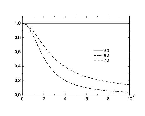
We set the parameters as λ1=0.1\lambda_{1}=0.1, λ2=1.0\lambda_{2}=1.0, λ3=1.0\lambda_{3}=1.0. For the five-dimensional case we have chosen ϕ⁡(0)=1.0\phi(0)=1.0, χ⁡(0)=0.6\chi(0)=\sqrt{0.6} and Λ=−3.6\Lambda=-3.6. For these parameters we solved the nonlinear eigenvalue problem for m1m_{1} and m2m_{2}. After 11 iterations, the eigenvalues m1≈1.989512m_{1}\approx 1.989512 and m2≈1.964764m_{2}\approx 1.964764 were found. In Fig. 1-4, we showed our numerical solutions. The spacetime is asymptotically an anti-de Sitter one: the asymptotic value of the potential (1) ϵ​V∞=ϵ⁡(λ2​m24/4+Λ)<0\epsilon V_{\infty}=\epsilon(\lambda_{2}m_{2}^{4}/4+\Lambda)<0 plays the role of a negative cosmological constant.

Refer to caption
Figure 1: The scalar field configurations ϕ\phi and χ\chi are shown as functions of the dimensionless rr.
Refer to caption
Figure 2: The metric function λ⁡(r)\lambda(r) is shown as functions of dimensionless rr.
Refer to caption
Figure 3: The function a′/aa^{\prime}/a is shown as functions of dimensionless rr.
Refer to caption
Figure 4: The energy density T00=ϵ⁡[12​λ​(ϕ′2+χ′2)+V]T_{0}^{0}=\epsilon\left[\frac{1}{2\lambda}\left(\phi^{\prime 2}+\chi^{\prime 2}\right)+V\right] is shown as functions of dimensionless rr.

For the six-dimensional case we take the boundary condition ϕ⁡(0)=3≈1.73205\phi(0)=\sqrt{3}\approx 1.73205 and χ⁡(0)=0.6≈0.774597\chi(0)=\sqrt{0.6}\approx 0.774597. We also choose the bulk cosmological constant as Λ=−λ2m24/4\Lambda=-\lambda_{2}m_{2}^{4}/4, in order for our solutions to be asymptotically flat in the bulk. After ten iterations, we find the eigenvalues m1≈2.3590m_{1}\approx 2.3590 and m2≈3.0599m_{2}\approx 3.0599. In Fig. 1-4 we showed our numerical solution for a given set of parameters.

As for the case of the seven-dimensional case we also choose the bulk cosmological constant as Λ=−λ2m24/4\Lambda=-\lambda_{2}m_{2}^{4}/4. After ten iterations, we find the eigenvalues m1≈2.24633m_{1}\approx 2.24633 and m2≈3.11911m_{2}\approx 3.11911. The obtained solutions for this case are presented in Figs. 1-4.

IV Stability

For stability analysis, let us write down the scalar field and Einstein equations, by keeping the time-dependence of the metric and field functions. Using the same rescaling as above and introducing new metric functions

a=eα,λ=eβ,a=e^{\alpha},\quad\lambda=e^{\beta},

one can get the following (r,t)(r,t) and (r,r)(r,r) components of the Einstein equations

3​α˙′−n+22​α′​β˙+n−12​β˙′=ϵ⁡[−ϕ˙​ϕ′−χ˙​χ′]​e2​β,\displaystyle 3\dot{\alpha}^{\prime}-\frac{n+2}{2}\alpha^{\prime}\dot{\beta}+\frac{n-1}{2}\dot{\beta}^{\prime}=\epsilon\left[-\dot{\phi}\phi^{\prime}-\dot{\chi}\chi^{\prime}\right]e^{2\beta}, (19)
(n−1)​{e−2​α​(α˙​β˙+12​(β¨+β˙2)+32​H​β˙)−2​(β′+2r)​α′​e−β−n−28​(β′+4r)​β′​e−β}−e−2​α​β˙2\displaystyle(n-1)\Big\{e^{-2\alpha}\Big(\dot{\alpha}\dot{\beta}+\frac{1}{2}\big(\ddot{\beta}+\dot{\beta}^{2}\big)+\frac{3}{2}H\dot{\beta}\Big)-2\big(\beta^{\prime}+\frac{2}{r}\big)\alpha^{\prime}e^{-\beta}-\frac{n-2}{8}\big(\beta^{\prime}+\frac{4}{r}\big)\beta^{\prime}e^{-\beta}\Big\}-e^{-2\alpha}\dot{\beta}^{2}
+\displaystyle+ 12e−2​α(α¨+α˙2+2−2αe2​α−β′2+3α˙)=ϵ[−12e2​α(ϕ˙2+χ˙2)−12eβ(ϕ+′2χ)′2+V].\displaystyle 12e^{-2\alpha}\big(\ddot{\alpha}+\dot{\alpha}^{2}+2-2\alpha{}^{\prime}{}^{2}e^{2\alpha-\beta}+3\dot{\alpha}\big)=\epsilon\Big[-\frac{1}{2}e^{2\alpha}\Big(\dot{\phi}^{2}+\dot{\chi}^{2}\Big)-\frac{1}{2}e^{\beta}\Big(\phi{}^{\prime}{}^{2}+\chi{}^{\prime}{}^{2}\Big)+V\Big]. (20)

Here the dot refers to derivative with respect to dimensionless time τ=H​t\tau=Ht. The scalar filed equations are:

e−2​α​ϕ¨−e−β​ϕ′′+e−2​α​(2​α˙+3+n​β˙2)​ϕ˙−e−β​(4​α′+n−1r+n−22​β′)​ϕ′=−ϕ⁡[2​λ3​χ2+λ1​(ϕ2−m12)],\displaystyle e^{-2\alpha}\ddot{\phi}-e^{-\beta}\phi^{\prime\prime}+e^{-2\alpha}\Big(2\dot{\alpha}+3+\frac{n\dot{\beta}}{2}\Big)\dot{\phi}-e^{-\beta}\Big(4\alpha^{\prime}+\frac{n-1}{r}+\frac{n-2}{2}\beta^{\prime}\Big)\phi^{\prime}=-\phi\Big[2\lambda_{3}\chi^{2}+\lambda_{1}\big(\phi^{2}-m_{1}^{2}\big)\Big]~, (21)
e−2​α​χ¨−e−β​χ′′+e−2​α​(2​α˙+3+n​β˙2)​χ˙−e−β​(4​α′+n−1r+n−22​β′)​χ′=−χ⁡[2​λ3​ϕ2+λ2​(χ2−m22)].\displaystyle e^{-2\alpha}\ddot{\chi}-e^{-\beta}\chi^{\prime\prime}+e^{-2\alpha}\Big(2\dot{\alpha}+3+\frac{n\dot{\beta}}{2}\Big)\dot{\chi}-e^{-\beta}\Big(4\alpha^{\prime}+\frac{n-1}{r}+\frac{n-2}{2}\beta^{\prime}\Big)\chi^{\prime}=-\chi\Big[2\lambda_{3}\phi^{2}+\lambda_{2}\big(\chi^{2}-m_{2}^{2}\big)\Big]~. (22)

Now we search for regular perturbed solutions of the above equations in the form

α\displaystyle\alpha =\displaystyle= α0​(r)+δ​α​(τ,r),β=β0​(r)+δ​β​(τ,r),\displaystyle\alpha_{0}(r)+\delta\alpha(\tau,r),\quad\beta=\beta_{0}(r)+\delta\beta(\tau,r),
ϕ\displaystyle\phi =\displaystyle= ϕ0​(r)+δ​ϕ​(τ,r),χ=χ0​(r)+δ​χ​(τ,r),\displaystyle\phi_{0}(r)+\delta\phi(\tau,r),\quad\chi=\chi_{0}(r)+\delta\chi(\tau,r), (23)

where the subscript 0 refers to static solutions of the equations and δ​α​(τ,r),δ​β​(τ,r),δ​ϕ​(τ,r),δ​χ​(τ,r)\delta\alpha(\tau,r),\delta\beta(\tau,r),\delta\phi(\tau,r),\delta\chi(\tau,r) are perturbations. Then we will have from (19) and (20):

3​(δ​α˙)′−n+22​α0′​δ​β˙+n−12​(δ​β˙)′=−ϵ⁡(δ​ϕ˙​ϕ0′+δ​χ˙​χ0′)​e2​β0,\displaystyle 3(\dot{\delta\alpha})^{\prime}-\frac{n+2}{2}\alpha_{0}^{\prime}\dot{\delta\beta}+\frac{n-1}{2}(\dot{\delta\beta})^{\prime}=-\epsilon\left(\dot{\delta\phi}\phi_{0}^{\prime}+\dot{\delta\chi}\chi_{0}^{\prime}\right)e^{2\beta_{0}}, (24)
(n−1){e−2​α02(δ​β¨+3δ​β˙)−2e−β0[−α0(β0+′2r)′δβ+(β0+′2r)δα+′α0δ′β]′\displaystyle(n-1)\Big\{\frac{e^{-2\alpha_{0}}}{2}\Big(\ddot{\delta\beta}+3\dot{\delta\beta}\Big)-2e^{-\beta_{0}}\Big[-\alpha_{0}{}^{\prime}\left(\beta_{0}{}^{\prime}+\frac{2}{r}\right)\delta\beta+\left(\beta_{0}{}^{\prime}+\frac{2}{r}\right)\delta\alpha{}^{\prime}+\alpha_{0}{}^{\prime}\delta\beta{}^{\prime}\Big]
−\displaystyle- n−28e−β0[−β0(β0+′4r)′δβ+2(β0+′2r)δβ]′}\displaystyle\frac{n-2}{8}e^{-\beta_{0}}\Big[-\beta_{0}{}^{\prime}\left(\beta_{0}{}^{\prime}+\frac{4}{r}\right)\delta\beta+2\left(\beta_{0}{}^{\prime}+\frac{2}{r}\right)\delta\beta{}^{\prime}\Big]\Big\}
+12​e−2​α0​[(δ​α¨+3​δ​α˙)−e−β0​(2​α0′​δ​α′−α0′2​δ​β−2​α0′2​δ​α)−4​δ​α]\displaystyle+12e^{-2\alpha_{0}}\left[\left(\ddot{\delta\alpha}+3\dot{\delta\alpha}\right)-e^{-\beta_{0}}\left(2\alpha_{0}^{\prime}\delta\alpha^{\prime}-\alpha_{0}^{\prime 2}\delta\beta-2\alpha_{0}^{\prime 2}\delta\alpha\right)-4\delta\alpha\right]
=ϵ[−eβ0(ϕ0δ′ϕ+′χ0δ′χ)′−eβ0​δ​β2(ϕ0+′2χ0)′2\displaystyle=\epsilon\Big[-e^{\beta_{0}}\big(\phi_{0}{}^{\prime}\delta\phi{}^{\prime}+\chi_{0}{}^{\prime}\delta\chi{}^{\prime}\big)-\frac{e^{\beta_{0}}\delta\beta}{2}\big(\phi_{0}{}^{\prime}{}^{2}+\chi_{0}{}^{\prime}{}^{2}\big)
+\displaystyle+ λ1ϕ0(ϕ02−m12)δϕ+λ2χ0(χ02−m22)δχ+2λ3ϕ02χ0δχ+2λ3χ02ϕ0δϕ],\displaystyle\lambda_{1}\phi_{0}\big(\phi_{0}^{2}-m_{1}^{2}\big)\delta\phi+\lambda_{2}\chi_{0}\big(\chi_{0}^{2}-m_{2}^{2}\big)\delta\chi+2\lambda_{3}\phi_{0}^{2}\chi_{0}\delta\chi+2\lambda_{3}\chi_{0}^{2}\phi_{0}\delta\phi\Big], (25)

and from (21) and (22) follows

e−2​α0(δ​ϕ¨+3δ​ϕ˙)−e−β0(δϕ−′′δβϕ0)′′−e−β0[(4α0+′n−22β0+′n−1r)(δϕ−′δβϕ0)′\displaystyle e^{-2\alpha_{0}}\big(\ddot{\delta\phi}+3\dot{\delta\phi}\big)-e^{-\beta_{0}}\big(\delta\phi{}^{\prime\prime}-\delta\beta\phi_{0}{}^{\prime\prime}\big)-e^{-\beta_{0}}\Big[\Big(4\alpha_{0}{}^{\prime}+\frac{n-2}{2}\beta_{0}{}^{\prime}+\frac{n-1}{r}\Big)\big(\delta\phi{}^{\prime}-\delta\beta\phi_{0}{}^{\prime}\big) (26)
+ϕ0(4δα+′n−22δβ)′′]=−4λ3ϕ0χ0δχ−[2λ3χ02+λ1(3ϕ02−m12)]δϕ,\displaystyle+\phi_{0}{}^{\prime}\Big(4\delta\alpha{}^{\prime}+\frac{n-2}{2}\delta\beta{}^{\prime}\Big)\Big]=-4\lambda_{3}\phi_{0}\chi_{0}\delta\chi-\Big[2\lambda_{3}\chi_{0}^{2}+\lambda_{1}\big(3\phi_{0}^{2}-m_{1}^{2}\big)\Big]\delta\phi,
e−2​α0(δ​χ¨+3δ​χ˙)−e−β0(δχ−′′δβχ0)′′−e−β0[(4α0+′n−22β0+′n−1r)(δχ−′δβχ0)′\displaystyle e^{-2\alpha_{0}}\big(\ddot{\delta\chi}+3\dot{\delta\chi}\big)-e^{-\beta_{0}}\big(\delta\chi{}^{\prime\prime}-\delta\beta\chi_{0}{}^{\prime\prime}\big)-e^{-\beta_{0}}\Big[\Big(4\alpha_{0}{}^{\prime}+\frac{n-2}{2}\beta_{0}{}^{\prime}+\frac{n-1}{r}\Big)\big(\delta\chi{}^{\prime}-\delta\beta\chi_{0}{}^{\prime}\big)
+\displaystyle+ χ0(4δα+′n−22δβ)′′]=−4λ3ϕ0χ0δϕ−[2λ3ϕ02+λ2(3χ02−m22)]δχ.\displaystyle\chi_{0}{}^{\prime}\Big(4\delta\alpha{}^{\prime}+\frac{n-2}{2}\delta\beta{}^{\prime}\Big)\Big]=-4\lambda_{3}\phi_{0}\chi_{0}\delta\phi-\left[2\lambda_{3}\phi_{0}^{2}+\lambda_{2}\left(3\chi_{0}^{2}-m_{2}^{2}\right)\right]\delta\chi~. (27)

One can see that Eqs. (24)-(26) contain similar terms like (δ​y¨+3​δ​y˙),\left(\ddot{\delta y}+3\dot{\delta y}\right), where δ​y\delta y is one of functions δ​α​(τ,r),δ​β​(τ,r),δ​φ​(τ,r),δ​χ​(τ,r)\delta\alpha(\tau,r),\delta\beta(\tau,r),\delta\varphi(\tau,r),\delta\chi(\tau,r). Such term implies that one can search for a solution in the form: δ​y=y1​(r)​e−32​τ​cos⁡ω​τ,{\delta y=y_{1}(r)e^{-\frac{3}{2}\tau}\cos{\omega\tau},} where ω=ω02−94>0\omega=\sqrt{\omega_{0}^{2}-\frac{9}{4}}>0. It implies that ω0>32\omega_{0}>\frac{3}{2}. Inserting the last expression into (24)-(26), one can get

3​α1′−n+22​α0′​β1+n−12​β1′=−ϵ⁡(ϕ0′​ϕ1+χ0′​χ1)​e2​β0,\displaystyle 3\alpha_{1}^{\prime}-\frac{n+2}{2}\alpha_{0}^{\prime}\beta_{1}+\frac{n-1}{2}\beta_{1}^{\prime}=-\epsilon\big(\phi_{0}^{\prime}\phi_{1}+\chi_{0}^{\prime}\chi_{1}\big)e^{2\beta_{0}}, (28)
(n−1){−e−2​α02ω02β1−2e−β0[−α0(β0+′2r)′β1+(β0+′2r)α1+′α0β1′]′\displaystyle(n-1)\Big\{-\frac{e^{-2\alpha_{0}}}{2}\omega_{0}^{2}\beta_{1}-2e^{-\beta_{0}}\Big[-\alpha_{0}{}^{\prime}\left(\beta_{0}{}^{\prime}+\frac{2}{r}\right)\beta_{1}+\left(\beta_{0}{}^{\prime}+\frac{2}{r}\right)\alpha_{1}{}^{\prime}+\alpha_{0}{}^{\prime}\beta_{1}{}^{\prime}\Big]
−\displaystyle- n−28e−β0[−β0(β0+′4r)′β1+2(β0+′2r)β1]′}+12e−2​α0[−ω02α1\displaystyle\frac{n-2}{8}e^{-\beta_{0}}\Big[-\beta_{0}{}^{\prime}\left(\beta_{0}{}^{\prime}+\frac{4}{r}\right)\beta_{1}+2\left(\beta_{0}{}^{\prime}+\frac{2}{r}\right)\beta_{1}{}^{\prime}\Big]\Big\}+12e^{-2\alpha_{0}}\Big[-\omega_{0}^{2}\alpha_{1}
−\displaystyle- e−β0(2α0′α1′−α0′2β1−2α0′2α1)−4α1]=ϵ[−eβ0(ϕ0ϕ1′+′χ0χ1′)′−eβ0​β12(ϕ0+′2χ0)′2\displaystyle e^{-\beta_{0}}\left(2\alpha_{0}^{\prime}\alpha_{1}^{\prime}-\alpha_{0}^{\prime 2}\beta_{1}-2\alpha_{0}^{\prime 2}\alpha_{1}\right)-4\alpha_{1}\Big]=\epsilon\Big[-e^{\beta_{0}}\big(\phi_{0}{}^{\prime}\phi_{1}{}^{\prime}+\chi_{0}{}^{\prime}\chi_{1}{}^{\prime}\big)-\frac{e^{\beta_{0}}\beta_{1}}{2}\big(\phi_{0}{}^{\prime}{}^{2}+\chi_{0}{}^{\prime}{}^{2}\big)
+\displaystyle+ λ1ϕ0(ϕ02−m12)ϕ1+λ2χ0(χ02−m22)χ1+2λ3ϕ02χ0χ1+2λ3χ02ϕ0ϕ1],\displaystyle\lambda_{1}\phi_{0}\big(\phi_{0}^{2}-m_{1}^{2}\big)\phi_{1}+\lambda_{2}\chi_{0}\big(\chi_{0}^{2}-m_{2}^{2}\big)\chi_{1}+2\lambda_{3}\phi_{0}^{2}\chi_{0}\chi_{1}+2\lambda_{3}\chi_{0}^{2}\phi_{0}\phi_{1}\Big], (29)

and

−e−2​α0ω02ϕ1−e−β0(ϕ1−′′β1ϕ0)′′−e−β0[(4α0+′n−22β0+′n−1r)(ϕ1−′β1ϕ0)′\displaystyle-e^{-2\alpha_{0}}\omega_{0}^{2}\phi_{1}-e^{-\beta_{0}}\big(\phi_{1}{}^{\prime\prime}-\beta_{1}\phi_{0}{}^{\prime\prime}\big)-e^{-\beta_{0}}\Big[\Big(4\alpha_{0}{}^{\prime}+\frac{n-2}{2}\beta_{0}{}^{\prime}+\frac{n-1}{r}\Big)\big(\phi_{1}{}^{\prime}-\beta_{1}\phi_{0}{}^{\prime}\big) (30)
+\displaystyle+ ϕ0(4α1+′n−22β1)′′]=−4λ3ϕ0χ0χ1−[2λ3χ02+λ1(3ϕ02−m12)]ϕ1,\displaystyle\phi_{0}{}^{\prime}\Big(4\alpha_{1}{}^{\prime}+\frac{n-2}{2}\beta_{1}{}^{\prime}\Big)\Big]=-4\lambda_{3}\phi_{0}\chi_{0}\chi_{1}-\Big[2\lambda_{3}\chi_{0}^{2}+\lambda_{1}\big(3\phi_{0}^{2}-m_{1}^{2}\big)\Big]\phi_{1},
−ω02e−2​α0χ1−e−β0(χ1−′′β1χ0)′′−e−β0[(4α0+′n−22β0+′n−1r)(χ1−′β1χ0)′\displaystyle-\omega_{0}^{2}e^{-2\alpha_{0}}\chi_{1}-e^{-\beta_{0}}\big(\chi_{1}{}^{\prime\prime}-\beta_{1}\chi_{0}{}^{\prime\prime}\big)-e^{-\beta_{0}}\Big[\Big(4\alpha_{0}{}^{\prime}+\frac{n-2}{2}\beta_{0}{}^{\prime}+\frac{n-1}{r}\Big)\big(\chi_{1}{}^{\prime}-\beta_{1}\chi_{0}{}^{\prime}\big)
+\displaystyle+ χ0(4α1+′n−22β1)′′]=−4λ3ϕ0χ0ϕ1−[2λ3ϕ02+λ2(3χ02−m22)]χ1.\displaystyle\chi_{0}{}^{\prime}\Big(4\alpha_{1}{}^{\prime}+\frac{n-2}{2}\beta_{1}{}^{\prime}\Big)\Big]=-4\lambda_{3}\phi_{0}\chi_{0}\phi_{1}-\Big[2\lambda_{3}\phi_{0}^{2}+\lambda_{2}\big(3\chi_{0}^{2}-m_{2}^{2}\big)\Big]\chi_{1}. (31)

So we have four usual differential equations for perturbations. For existence of stable solutions we need to provide positiveness of an eigenvalue ω02\omega_{0}^{2}. To do this we will search for finite solutions of above equations.

For the five-dimensional model, by setting β1=0\beta_{1}=0 (and β0=0\beta_{0}=0) and substituting n=1n=1, the perturbations equations are simply reduced to

ϕ1+′′4α0ϕ1′−′[2λ3χ02+4​ϵ3ϕ0+′2λ1(3ϕ02−m12)]ϕ1−(4​ϵ3ϕ0χ0′+′4λ3ϕ0χ0)χ1+ω02e−2​α0ϕ1=0,\displaystyle\phi_{1}{}^{\prime\prime}+4\alpha_{0}{}^{\prime}\phi_{1}{}^{\prime}-\Big[2\lambda_{3}\chi_{0}^{2}+\frac{4\epsilon}{3}\phi_{0}{}^{\prime}{}^{2}+\lambda_{1}\left(3\phi_{0}^{2}-m_{1}^{2}\right)\Big]\phi_{1}-\Big(\frac{4\epsilon}{3}\phi_{0}{}^{\prime}\chi_{0}{}^{\prime}+4\lambda_{3}\phi_{0}\chi_{0}\Big)\chi_{1}+\omega_{0}^{2}e^{-2\alpha_{0}}\phi_{1}=0,
χ1+′′4α0χ1′−′[2λ3ϕ02+4​ϵ3χ0+′2λ2(3χ02−m22)]χ1−(4​ϵ3ϕ0χ0′+′4λ3ϕ0χ0)ϕ1+ω02e−2​α0χ1=0,\displaystyle\chi_{1}{}^{\prime\prime}+4\alpha_{0}{}^{\prime}\chi_{1}{}^{\prime}-\Big[2\lambda_{3}\phi_{0}^{2}+\frac{4\epsilon}{3}\chi_{0}{}^{\prime}{}^{2}+\lambda_{2}\left(3\chi_{0}^{2}-m_{2}^{2}\right)\Big]\chi_{1}-\Big(\frac{4\epsilon}{3}\phi_{0}{}^{\prime}\chi_{0}{}^{\prime}+4\lambda_{3}\phi_{0}\chi_{0}\Big)\phi_{1}+\omega_{0}^{2}e^{-2\alpha_{0}}\chi_{1}=0, (32)

where we have used Eq. (28)

3​α1′=−ϵ⁡(ϕ0′​ϕ1+χ0′​χ1)3\alpha_{1}^{\prime}=-\epsilon\left(\phi_{0}^{\prime}\phi_{1}+\chi_{0}^{\prime}\chi_{1}\right)

to eliminate α1′\alpha_{1}{}^{\prime}. We solved numerically the Eqs. (32), using the background solutions obtained in Sec. III, with the boundary conditions

ϕ1​(0)=1.0,ϕ1′​(0)=0.0,χ1​(0)=−1.0,χ1′​(0)=0.0,ϕ1​(r→∞)→0,χ1​(r→∞)→0.\displaystyle\phi_{1}(0)=1.0,\quad\phi_{1}^{\prime}(0)=0.0,\quad\chi_{1}(0)=-1.0,\quad\chi_{1}^{\prime}(0)=0.0,\quad\phi_{1}(r\to\infty)\to 0,\quad\chi_{1}(r\to\infty)\to 0. (33)

In the case of the thick Minkowski brane solutions supported by the phantom scalar fields, it has been shown that these solutions are stable [6]. In our case, the perturbation equations also have regular solutions. Also, we have confirmed that there are no solutions with ω02<0\omega_{0}^{2}<0, i.e. unstable solutions are absent. In Fig 5, we showed an example of numerical solutions for perturbations with ω0≈13.179575\omega_{0}\approx 13.179575. We conclude that our thick de Sitter brane solutions supported by the phantom scalar fields are stable, irrespectively of the value of the Hubble parameter HH. As a special limit H→0H\to 0, we may recover the result for the Minkowski brane solutions.

Refer to caption
Figure 5: The perturbed scalar field configurations ϕ1\phi_{1} (solid curve) and χ1\chi_{1} for ω0≈13.179575\omega_{0}\approx 13.179575 (dashed-dotted curve) are shown as functions of rr. As the background solutions, we used the one shown in Figs. 1-3.

It is also reasonable to expect that our phantom thick brane solutions in six- and seven-dimensional spacetime are also completely stable, since the spacetime structures of higher-dimensional solutions are essentially very similar to that of the five-dimensional solution.

V Summary and Discussions

In this paper, we have presented five-, six-, and seven-dimensional thick de Sitter brane solutions supported by two interacting (phantom) scalar fields. The special form of the potential (1) allows us to find regular solutions with finite energy density. It was shown that asymptotically there exist anti-de Sitter spacetime for the five-dimensional case and flat spacetime for the six- and seven-dimensional cases.

Also we have investigated the stability of our thick brane solutions. In the five-dimensional thick de Sitter brane solutions, we have shown the presence of decaying solutions for perturbations. We also could not find any mode with negative eigenvalue. This, of course, implies that our solutions in five-dimensional spacetime are stable. It is also quite reasonable to expect that our thick brane solutions in higher dimensions are also stable since the spacetime and vacuum structures are essentially the same as in the case of five spacetime dimensions.

Acknowledgements

The work of M. M. was supported by the project TRR 33 The Dark Universe at the ASC. VD is grateful to the Alexander von Humboldt Foundation for financial support and to V. Mukhanov for invitation to Universitaet Muenchen for research. This work was supported by the Korea Science and Engineering Foundation(KOSEF) grant funded by the Korea government(MEST) through the Center for Quantum Spacetime(CQUeST) of Sogang University with grant number R11 - 2005 - 021.

References

  • [1] L. Randall and R. Sundrum, Phys. Rev. Lett. 83, 3370 (1999) [arXiv:hep-ph/9905221]; L. Randall and R. Sundrum, Phys. Rev. Lett. 83, 4690 (1999) [arXiv:hep-th/9906064].
  • [2] R. Maartens, Living Rev. Rel. 7, 7 (2004) [arXiv:gr-qc/0312059]l P. Brax, C. van de Bruck and A. C. Davis, Rept. Prog. Phys. 67, 2183 (2004) [arXiv:hep-th/0404011].
  • [3] O. DeWolfe, D. Z. Freedman, S. S. Gubser and A. Karch, Phys. Rev. D 62, 046008 (2000) [arXiv:hep-th/9909134]; M. Gremm, Phys. Lett. B 478, 434 (2000) [arXiv:hep-th/9912060]; C. Csaki, J. Erlich, T. J. Hollowood and Y. Shirman, Nucl. Phys. B 581, 309 (2000) [arXiv:hep-th/0001033]; M. Giovannini, Phys. Rev. D 65, 064008 (2002) [arXiv:hep-th/0106131].
  • [4] S. Kobayashi, K. Koyama and J. Soda, Phys. Rev. D 65, 064014 (2002) [arXiv:hep-th/0107025]. N. Sasakura, JHEP 0202, 026 (2002) [arXiv:hep-th/0201130]; N. Sasakura, Phys. Rev. D 66, 065006 (2002) [arXiv:hep-th/0203032]; A. Z. Wang, Phys. Rev. D 66, 024024 (2002) [arXiv:hep-th/0201051]; K. A. Bronnikov and B. E. Meierovich, Grav. Cosmol. 9, 313 (2003) [arXiv:gr-qc/0402030]; M. Minamitsuji, W. Naylor and M. Sasaki, Nucl. Phys. B 737, 121 (2006) [arXiv:hep-th/0508093]; M. Minamitsuji, W. Naylor and M. Sasaki, Phys. Lett. B 633, 607 (2006) [arXiv:hep-th/0510117]; N. Barbosa-Cendejas and A. Herrera-Aguilar, Phys. Rev. D 73, 084022 (2006) [Erratum-ibid. D 77, 049901 (2008)] [arXiv:hep-th/0603184].
  • [5] V. Dzhunushaliev, Grav. Cosmol. 13, 302 (2007) [arXiv:gr-qc/0603020];
  • [6] V. Dzhunushaliev, V. Folomeev, S. Myrzakul and R. Myrzakulov, arXiv:0804.0151 [gr-qc].
  • [7] V. Dzhunushaliev, V. Folomeev, K. Myrzakulov and R. Myrzakulov, arXiv:0705.4014 [gr-qc]; V. Dzhunushaliev, V. Folomeev, D. Singleton and S. Aguilar-Rudametkin, Phys. Rev. D 77, 044006 (2008) [arXiv:hep-th/0703043].
  • [8] M. Giovannini, H. Meyer and M. E. Shaposhnikov, Nucl. Phys. B 619, 615 (2001) [arXiv:hep-th/0104118]; T. Gherghetta, E. Roessl and M. E. Shaposhnikov, Phys. Lett. B 491, 353 (2000) [arXiv:hep-th/0006251]. R. S. Torrealba S., arXiv:0803.0313 [hep-th].
  • [9] V. Dzhunushaliev, arXiv:hep-ph/0605070.
  • [10] W. Heisenberg, Introduction to the unified field theory of elementary particles., (Max - Planck - Institut für Physik und Astrophysik, Interscience Publishers London, New York-Sydney, 1966).
  • [11] D. Singleton, Phys.Rev. D70, 065013 (2004).