跳到论文正文
W Papers独立论文阅读器 arXiv:0809.3975 论文正文 计算阅读时间 · 0%
引用这篇论文根据当前论文元数据生成,正式投稿前建议核对。


License: arXiv.org perpetual non-exclusive license
arXiv:0809.3975v2 [quant-ph] 04 Dec 2008

Van der Waals potentials of paramagnetic atoms

Hassan Safari Affiliation: Theoretisch-Physikalisches Institut, Friedrich-Schiller-Universität Jena, Max-Wien-Platz 1, 07743 Jena, Germany    Dirk-Gunnar Welsch Affiliation: Theoretisch-Physikalisches Institut, Friedrich-Schiller-Universität Jena, Max-Wien-Platz 1, 07743 Jena, Germany    Stefan Yoshi Buhmann Affiliation: Quantum Optics and Laser Science, Blackett Laboratory, Imperial College London, Prince Consort Road, London SW7 2BW, United Kingdom    Stefan Scheel Affiliation: Quantum Optics and Laser Science, Blackett Laboratory, Imperial College London, Prince Consort Road, London SW7 2BW, United Kingdom
August 24, 2026
Abstract

We study single- and two-atom van der Waals interactions of ground-state atoms which are both polarizable and paramagnetizable in the presence of magnetoelectric bodies within the framework of macroscopic quantum electrodynamics. Starting from an interaction Hamiltonian that includes particle spins, we use leading-order perturbation theory to express the van der Waals potentials in terms of the polarizability and magnetizability of the atom(s). To allow for atoms embedded in media, we also include local-field corrections via the real-cavity model. The general theory is applied to the potential of a single atom near a half space and that of two atoms embedded in a bulk medium or placed near a sphere, respectively.

pacs
34.35.+a, 34.20.–b 42.50.Nn

I Introduction

The dispersion interaction between neutral and (unpolarized) atoms or molecules — commonly known as the van der Waals (vdW) interaction — is, together with Casimir-Polder and Casimir forces, one of the consequences of zero-point fluctuations in quantum electrodynamics (QED) (for a recent review, see Ref. [1]). The interaction potential of two polarizable atoms in free space was first studied for small distances (nonretarded limit) by London using second-order perturbation theory [2]. In this limit the result is an attractive potential proportional to r−6r^{-6} with rr being the interatomic distance. The London formula was extended to arbitrary distances by Casimir and Polder using fourth-order perturbation theory within the framework of QED [3]. They found an attractive potential proportional to r−7r^{-7} for large separations (retarded limit) where the potential is due to the ground-state fluctuations of both the atomic dipole moments and the electromagnetic far field. Casimir and Polder also considered the potential of a polarizable atom in the presence of a perfectly conducting wall [3]. The result is an attractive potential which shows a z−3z^{-3} dependence in the nonretarded limit and is proportional to z−4z^{-4} in the retarded limit (zz being the atom-wall separation).

In the three-atom case, a nonadditive term prevents the potential from just being the sum of three pairwise contributions; it was first calculated in the nonretarded limit [4, 5] and extended to arbitrary interatomic distances [6]. Later, a general formula for the nonadditive NN-atom vdW potential was obtained by summing the responses of each atom to the electromagnetic field of produced by the other atoms [7], or alternatively, by calculating the zero-point energy difference of the electromagnetic field with and without the atoms [8].

The theory was first extended to magnetic atoms by Feinberg and Sucher [9] who studied the retarded interaction of two electromagnetic atoms based on a calculation of photon scattering amplitudes; their results were later reproduced by Boyer [10] using a zero-point energy technique. In this limit, the interaction potential of a polarizable atom and a magnetizable one was found to be repulsive and proportional to r−7r^{-7}. Later on, Feinberg and Sucher extended their formula to arbitrary distances [11]. In particular, in the nonretarded limit the potential of the mentioned atoms is found to be repulsive and proportional to r−4r^{-4}. The retarded Feinberg–Sucher potential was extended to atoms with crossed electric-magnetic polarizabilities on the basis of a duality argument [12]. For the single-atom case, the atom-wall potential, calculated in Ref. [3] in the retarded limit, has been generalized to atoms with both electric and magnetic polarizabilities [10], showing that a magnetically polarizable atom in a distance ll from a conducting wall is repelled by that wall due to a potential proportional to l−4l^{-4}. A full QED treatment has been invoked to study the potential of an excited magnetic atom placed inside a planar cavity for all distance regimes [13].

In order to extend the theory of atom–atom interactions to the case of magnetoelectrics being present, the effect of the bodies on the fluctuating electromagnetic field must be taken into account. A general formula expressing the vdW potential between two polarizable ground-state atoms in the presence of electric bodies in terms of the Green tensor of the body-assisted electromagnetic field was first obtained using linear response theory [14] and later reproduced by treating the effect of the bodies semiclassically [15]. Recently, an analogous formula for two polarizable atoms interacting in the presence of magnetoelectric bodies was derived by using fourth-order perturbation theory within the framework of macroscopic QED [16], it was later generalized to NN atoms [17]. For atoms that are embedded in a host body or medium, the local electromagnetic field experienced by them differs from the macroscopic one. Hence, the theory of vdW interactions must be modified by taking local-field corrections into account. One approach to this problem is the real-cavity model, where one assumes that each guest atom is surrounded by a small, empty, spherical cavity [18]. It has been used to study local-field corrections to the spontaneous decay rate of an atom embedded in an arrangement of magnetoelectric bodies and/or media [19] and was recently applied to obtain local-field corrected formulas for one-atom and two-atom vdW potentials of polarizable atoms within such geometries [20].

In this article, we generalize the theory of ground-state single- and two-atom vdW potentials in the presence of arbitrarily shaped magnetoelectric bodies to atoms exhibiting both polarizabilities and (para-) magnetizabilities. Such a theory includes and generalizes the recently studied potential of two polarizable and magnetizable bodies embedded in a bulk magnetoelectric medium [21]. This article is organized as follows. In Sec. II, the multipolar atom–field interaction Hamiltonian is derived for atoms that are both electric and (para)magnetic. In Sec. III, general expressions for single- and two-atom potentials are derived using perturbation theory. Local-field corrections are considered in Sec. IV, while in Sec. V, we apply our theory by studying the examples of (i) an atom in the presence of a half space, (ii) two atoms in bulk media, and (iii) two atoms in the presence of a sphere. A summary is given in Sec. VI.

II Atom–field interactions in the presence of spins

The interaction of individual atoms with medium-assisted electromagnetic fields has extensively been discussed for spinless atoms [22, 23, 16, 24]. In order to correctly describe the paramagnetic properties of an atom, it is crucial to include the spins of its constituents in the considerations. A neutral atom (or molecule) AA thus has to be regarded as being a collection of (nonrelativistic) particles α∈A\alpha\in A which in addition to their charges qαq_{\alpha} (∑α∈Aqα=0\sum_{\alpha\in A}q_{\alpha}=0), masses mαm_{\alpha}, positions 𝒓^α\hat{\bm{r}}_{\alpha}, canonically conjugate momenta 𝒑^α\hat{\bm{p}}_{\alpha} have spins 𝒔^α\hat{\bm{s}}_{\alpha}. The particle spins give rise to magnetic dipole moments γα​𝒔^α\gamma_{\alpha}\hat{\bm{s}}_{\alpha}, where γα\gamma_{\alpha} is the gyromagnetic ratio of particle α\alpha [γe=−ege/(2me)\gamma_{e}=-eg_{e}/(2m_{e}) for electrons with −e-e: electron charge; ge≃2g_{e}\simeq 2, electron gg-factor; mem_{e}: electron mass]. While leaving the atomic charge density

ρ^A​(𝒓)=∑α∈Aqα​δ​(𝒓−𝒓^α)\hat{\rho}_{A}(\bm{r})=\sum_{\alpha\in A}q_{\alpha}\delta(\bm{r}-\hat{\bm{r}}_{\alpha}) (1)

and polarization

𝑷^A​(𝒓)=∑α∈Aqα​𝒓¯^α​∫01d​σ​δ​(𝒓−𝒓^A−σ​𝒓¯^α)\hat{\bm{P}}_{A}(\bm{r})=\sum_{\alpha\in A}q_{\alpha}\hat{\overline{\bm{r}}}_{\alpha}\int_{0}^{1}\mathrm{d}\sigma\,\delta\!\left(\bm{r}-\hat{\bm{r}}_{A}-\sigma\hat{\overline{\bm{r}}}_{\alpha}\right) (2)

unaffected, the spin magnetic momentsdo contribute to the atomic current density and magnetization, so that the expressions given in Refs. [23, 24] for spinless particles generalize to

𝒋^A​(𝒓)=\displaystyle\hat{\bm{j}}_{A}(\bm{r})= ∑α∈Aqα2​[𝒓^˙α​δ​(𝒓−𝒓^α)+δ⁡(𝒓−𝒓^α)​𝒓^˙α]\displaystyle\sum_{\alpha\in A}\frac{q_{\alpha}}{2}\left[\dot{\hat{\bm{r}}}_{\alpha}\delta(\bm{r}-\hat{\bm{r}}_{\alpha})+\delta(\bm{r}-\hat{\bm{r}}_{\alpha})\dot{\hat{\bm{r}}}_{\alpha}\right]
−∑α∈Aγα𝒔^α×∇δ(𝒓−𝒓^α)\displaystyle-\sum_{\alpha\in A}\gamma_{\alpha}\hat{\bm{s}}_{\alpha}\times\bm{\nabla}\delta(\bm{r}-\hat{\bm{r}}_{\alpha}) (3)

and

𝑴^A(𝒓)=∑α∈Aqα2∫01dσσ[δ(𝒓−𝒓^A−σ𝒓¯^α)𝒓¯^α×𝒓¯^˙α−𝒓¯^˙α×𝒓¯^αδ(𝒓−𝒓^A−σ𝒓¯^α)]+∑α∈Aγα𝒔^αδ(𝒓−𝒓^α).\!\!\hat{\bm{M}}_{A}(\bm{r})=\sum_{\alpha\in A}\frac{q_{\alpha}}{2}\int_{0}^{1}\mathrm{d}\sigma\,\sigma\left[\delta\left(\bm{r}-\hat{\bm{r}}_{A}-\sigma\hat{\overline{\bm{r}}}_{\alpha}\right)\hat{\overline{\bm{r}}}_{\alpha}\times\dot{\hat{\overline{\bm{r}}}}_{\alpha}\right.\\ \quad\left.-\dot{\hat{\overline{\bm{r}}}}_{\alpha}\times\hat{\overline{\bm{r}}}_{\alpha}\delta\left(\bm{r}-\hat{\bm{r}}_{A}-\sigma\hat{\overline{\bm{r}}}_{\alpha}\right)\right]+\sum_{\alpha\in A}\gamma_{\alpha}\hat{\bm{s}}_{\alpha}\delta(\bm{r}-\hat{\bm{r}}_{\alpha}). (4)

In Eqs. (2) and (4), 𝒓¯^α\hat{\overline{\bm{r}}}_{\alpha} =\!= 𝒓^α\!\hat{\bm{r}}_{\alpha} −\!- 𝒓^A\!\hat{\bm{r}}_{\!A} denotes the position of the α\alphath particle relative to the center-of-mass position

𝒓^A=∑α∈AmαmA​𝒓^α\hat{\bm{r}}_{A}=\sum_{\alpha\in A}\frac{m_{\alpha}}{m_{A}}\,\hat{\bm{r}}_{\alpha} (5)

(mAm_{A} =\!= ∑α∈Amα\!\sum_{\alpha\in A}m_{\alpha}), with the associated momenta being

𝒑¯^α=𝒑^α−mαmA​𝒑^A\hat{\bar{\bm{p}}}_{\alpha}=\hat{\bm{p}}_{\alpha}-\frac{m_{\alpha}}{m_{A}}\hat{\bm{p}}_{A} (6)

and 𝒑^A\hat{\bm{p}}_{A} =\!= ∑α∈A𝒑^α\!\sum_{\alpha\in A}\hat{\bm{p}}_{\alpha}, respectively. Since the current density associated with the spins is transverse, the continuity equation ρ^˙A+∇⋅𝒋^A=0\dot{\hat{\rho}}_{A}+\bm{\nabla}\cdot\hat{\bm{j}}_{A}=0 remains valid. In addition, the atomic charge and current densities can still be related to the atomic polarization and magnetization via

ρ^A=−∇⋅𝑷^A,\displaystyle\hat{\rho}_{A}=-\bm{\nabla}\cdot\hat{\bm{P}}_{A}\;, (7)
𝒋^A=𝑷^˙A+∇×𝑴^A+𝒋^Ro\displaystyle\hat{\bm{j}}_{A}=\dot{\hat{\bm{P}}}_{A}+\bm{\nabla}\times\hat{\bm{M}}_{A}+\hat{\bm{j}}_{\mathrm{Ro}} (8)

as in the case of spinless particles, since the particle spins lead to equal contributions on the left and right hand sides of Eq. (8), as an inspection of Eqs. (3) and (4) shows. In Eq. (8),

𝒋^Ro=12∇×[𝑷^A×𝒓^˙A−𝒓^˙A×𝑷^A]\hat{\bm{j}}_{\mathrm{Ro}}={\textstyle\frac{1}{2}}\,\bm{\nabla}\times\left[\hat{\bm{P}}_{A}\times\dot{\hat{\bm{r}}}_{A}-\dot{\hat{\bm{r}}}_{A}\times\hat{\bm{P}}_{A}\right] (9)

is the Röntgen current density associated with the center-of-mass motion of the atom [25, 26]. Further atomic quantities of interest are the atomic electric and magnetic dipole moments

𝒅^A=∑α∈Aqα𝒓¯^α=∑α∈Aqα𝒓^α\hat{\bm{d}}_{A}=\sum_{\alpha\in A}q_{\alpha}\hat{\overline{\bm{r}}}{}_{\alpha}=\sum_{\alpha\in A}q_{\alpha}\hat{\bm{r}}_{\alpha} (10)

and

𝒎^A=∑α∈A[qα2​𝒓¯^α×𝒓¯^˙α+γα​𝒔^α],\hat{\bm{m}}_{A}=\sum_{\alpha\in A}\left[\frac{q_{\alpha}}{2}\,\hat{\overline{\bm{r}}}_{\alpha}\times\dot{\hat{\overline{\bm{r}}}}_{\alpha}+\gamma_{\alpha}\hat{\bm{s}}_{\alpha}\right], (11)

which emerge from the atomic polarization (2) and magnetization (4) in the long-wavelength approximation, as we will see later on. The first and second terms in Eq. (11) obviously represent the orbital angular momentum and spin contributions to the magnetic dipole moment.

In order to account for the interaction of the spins with the magnetic field, a Pauli term has to be included in the minimal-coupling Hamiltonian given in Ref. [16] for spinless atoms interacting with the quantized electromagnetic field in the presence of linearly responding magnetoelectric bodies, viz.,

H^=\displaystyle\hat{H}= ∑λ=e,m∫d3​r​∫0∞d​ω​ℏ​ω​𝒇^λ†​(𝒓,ω)⋅𝒇^λ​(𝒓,ω)\displaystyle\sum_{\lambda=e,m}\int\mathrm{d}^{3}r\int_{0}^{\infty}\mathrm{d}\omega\,\hbar\omega\,\hat{\bm{f}}_{\lambda}^{\dagger}(\bm{r},\omega)\cdot\hat{\bm{f}}_{\lambda}(\bm{r},\omega)
+∑α∈∪A[𝒑^α−qα​𝑨^​(𝒓^α)]22​mα+∑α,β∈∪Aα≠βqα​qβ8​π​ε0​|𝒓^α−𝒓^β|\displaystyle+\sum_{\alpha\in\cup A}\frac{\left[\hat{\bm{p}}_{\alpha}-q_{\alpha}\hat{\bm{A}}(\hat{\bm{r}}_{\alpha})\right]^{2}}{2m_{\alpha}}+\sum_{\begin{subarray}{c}\alpha,\beta\in\cup A\\ \alpha\neq\beta\end{subarray}}\frac{q_{\alpha}q_{\beta}}{8\pi\varepsilon_{0}|\hat{\bm{r}}_{\alpha}-\hat{\bm{r}}_{\beta}|}
+∑α∈∪Aqαφ^(𝒓^α)−∑α∈∪Aγα𝒔^α⋅𝑩^(𝒓^α).\displaystyle+\sum_{\alpha\in\cup A}q_{\alpha}\hat{\varphi}(\hat{\bm{r}}_{\alpha})-\sum_{\alpha\in\cup A}\gamma_{\alpha}\hat{\bm{s}}_{\alpha}\!\cdot\!\hat{\bm{B}}(\hat{\bm{r}}_{\alpha})\,. (12)

The first term in Eq. (12) is the energy of the electromagnetic field and the bodies, expressed in terms of bosonic (collective) variables 𝒇^λ​(𝒓,ω)\hat{\bm{f}}_{\lambda}(\bm{r},\omega) and 𝒇^λ†​(𝒓,ω)\hat{\bm{f}}_{\lambda}^{\dagger}(\bm{r},\omega) (λ\lambda, λ′\!\lambda^{\prime} ∈\!\in {e,m}\!\{e,m\}, with ee, mm denoting electric and magnetic excitations), the second term is the kinetic energy of the charged particles constituting the atoms, the third and fourth terms denote their mutual and body-assisted Coulomb potentials, respectively, and the last term is the newly introduced Pauli interaction of the particle spins with the body-assisted magnetic field. Note that the scalar potential φ^\hat{\varphi}, the vector potential 𝑨^\hat{\bm{A}}, and the induction field 𝑩^\hat{\bm{B}} are thought of as being expressed in terms of the fundamental bosonic fields 𝒇^λ\hat{\bm{f}}_{\lambda} and 𝒇^λ†\hat{\bm{f}}_{\lambda}^{\dagger} [27, 24].

To verify the consistency of the Hamiltonian (12), we need to show that it leads to the correct Maxwell equations for the electromagnetic field and the Newton equations for the particles. As in the case of spinless particles, the total electromagnetic field can be given by

𝓔^=𝑬^−∑A∇φ^A,\displaystyle\hat{\bm{\mathcal{E}}}=\hat{\bm{E}}-\sum_{A}\bm{\nabla}\hat{\varphi}_{A},\quad 𝓑^=𝑩^,\displaystyle\hat{\bm{\mathcal{B}}}=\hat{\bm{B}}, (13)
𝓓^=𝑫^−ε0​∑A∇φ^A,\displaystyle\hat{\bm{\mathcal{D}}}=\hat{\bm{D}}-\varepsilon_{0}\sum_{A}\bm{\nabla}\hat{\varphi}_{A},\quad 𝓗^=𝑯^,\displaystyle\hat{\bm{\mathcal{H}}}=\hat{\bm{H}}, (14)

where 𝑬^\hat{\bm{E}}, 𝑩^\hat{\bm{B}}, 𝑫^\hat{\bm{D}} and 𝑯^\hat{\bm{H}} are the body-assisted electromagnetic-field strengths [27, 24], and

φ^A​(𝒓)=∑α∈Aqα4​π​ε0​|𝒓−𝒓^α|\hat{\varphi}_{A}(\bm{r})=\sum_{\alpha\in A}\frac{q_{\alpha}}{4\pi\varepsilon_{0}|\bm{r}-\hat{\bm{r}}_{\alpha}|} (15)

is the Coulomb potential due to atom AA. Since the atomic charge density (1) is not affected by the particle spins either, the Maxwell equations

∇⋅𝓑^=0,\displaystyle\bm{\nabla}\cdot\hat{\bm{\mathcal{B}}}=0, (16)
∇⋅𝓓^=∑Aρ^A,\displaystyle\bm{\nabla}\cdot\hat{\bm{\mathcal{D}}}=\sum_{A}\hat{\rho}_{A}, (17)

which are not governed by the system Hamiltonian, are not changed by the presence of spins. It is obvious that the Maxwell equation

∇×𝓔^+𝓑^˙=0\bm{\nabla}\times\hat{\bm{\mathcal{E}}}+\dot{\hat{\bm{\mathcal{B}}}}=\mbox{{{0}}} (18)

also remains unchanged, because the Pauli interaction term commutes with the 𝓑^\hat{\bm{\mathcal{B}}}-field and hence its inclusion does not lead to an additional contribution in Heisenberg’s equation of motion 𝓑^˙\dot{\hat{\bm{\mathcal{B}}}} =\!= (i/ℏ)​[H^,𝓑^]\!(\mathrm{i}/\hbar)\left[\hat{H},\hat{\bm{\mathcal{B}}}\right]. As implied by the commutation relation [27]

[D^i​(𝒓),A^j​(𝒓′)]=i​ℏ​δi​j⟂​(𝒓−𝒓′)\left[\hat{D}_{i}(\bm{r}),\hat{A}_{j}(\bm{r}^{\prime})\right]=\mathrm{i}\hbar\delta^{\perp}_{ij}(\bm{r}-\bm{r}^{\prime}) (19)

[δi​j⟂​(𝒓)\delta^{\perp}_{ij}(\bm{r}), transverse delta function], the Pauli interaction does lead to an additional contribution

iℏ[−∑α∈∪Aγα𝒔^α⋅𝑩^(𝒓^α),𝑫^(𝒓)]=−∑α∈∪Aγα𝒔^α×∇δ(𝒓−𝒓^α)\frac{\mathrm{i}}{\hbar}\Biggl[-\sum_{\alpha\in\cup A}\gamma_{\alpha}\hat{\bm{s}}_{\alpha}\cdot\hat{\bm{B}}(\hat{\bm{r}}_{\alpha}),\hat{\bm{D}}(\bm{r})\Biggr]\\ =-\sum_{\alpha\in\cup A}\gamma_{\alpha}\hat{\bm{s}}_{\alpha}\times\bm{\nabla}\delta(\bm{r}-\hat{\bm{r}}_{\alpha}) (20)

in the Heisenberg equation of motion 𝓓^˙\dot{\hat{\bm{\mathcal{D}}}} =\!= (i/ℏ)​[H^,𝓓^]\!(\mathrm{i}/\hbar)\bigl[\hat{H},\hat{\bm{\mathcal{D}}}\bigr], which coincides with the spin-induced component of 𝒋^A\hat{\bm{j}}_{A} [second term in Eq. (3)]. Hence, the Maxwell equation

∇×𝓗^−𝓓^˙=∑A𝒋^A\displaystyle\bm{\nabla}\times\hat{\bm{\mathcal{H}}}-\dot{\hat{\bm{\mathcal{D}}}}=\sum_{A}\hat{\bm{j}}_{A} (21)

holds in the presence of spin when using the amended atomic current density (3).

Next, consider the equations of motion for the charged particles. Using the Hamiltonian (12), we have

𝒓^˙α=1mα​[𝒑^α−qα​𝑨^​(𝒓^α)],\dot{\hat{\bm{r}}}_{\alpha}=\frac{1}{m_{\alpha}}\left[\hat{\bm{p}}_{\alpha}-q_{\alpha}\hat{\bm{A}}(\hat{\bm{r}}_{\alpha})\right], (22)

as in the absence of spins. Equation (22) implies that the Pauli interaction gives rise to a contribution

iℏ[−∑β∈∪Aγβ𝒔^β⋅𝑩^(𝒓^β),mα𝒓^˙α]=γα∇α[𝒔^α⋅𝑩^(𝒓^α)]\frac{\mathrm{i}}{\hbar}\left[-\sum_{\beta\in\cup A}\gamma_{\beta}\hat{\bm{s}}_{\beta}\cdot\hat{\bm{B}}(\hat{\bm{r}}_{\beta}),m_{\alpha}\dot{\hat{\bm{r}}}_{\alpha}\right]=\gamma_{\alpha}\bm{\nabla}_{\alpha}\left[\hat{\bm{s}}_{\alpha}\cdot\hat{\bm{B}}(\hat{\bm{r}}_{\alpha})\right] (23)

to mα​𝒓^¨α=(i/ℏ)​[H^,mα​𝒓^˙α]m_{\alpha}\ddot{\hat{\bm{r}}}_{\alpha}=(\mathrm{i}/\hbar)\left[\hat{H},m_{\alpha}\dot{\hat{\bm{r}}}_{\alpha}\right]. Combining this with the contributions from the spin-independent part of the Hamiltonian [27], we arrive at

mα​𝒓^¨α=\displaystyle m_{\alpha}\ddot{\hat{\bm{r}}}_{\alpha}= qα​𝓔^​(𝒓^α)+qα2​[𝒓^˙α×𝓑^​(𝒓^α)−𝓑^​(𝒓^α)×𝒓^˙α]\displaystyle q_{\alpha}\hat{\bm{\mathcal{E}}}(\hat{\bm{r}}_{\alpha})+\frac{q_{\alpha}}{2}\left[\dot{\hat{\bm{r}}}_{\alpha}\times\hat{\bm{\mathcal{B}}}(\hat{\bm{r}}_{\alpha})-\hat{\bm{\mathcal{B}}}(\hat{\bm{r}}_{\alpha})\times\dot{\hat{\bm{r}}}_{\alpha}\right]
+γα​∇α[𝒔^α⋅𝓑^​(𝒓^α)].\displaystyle+\gamma_{\alpha}\bm{\nabla}_{\alpha}\left[\hat{\bm{s}}_{\alpha}\cdot\hat{\bm{\mathcal{B}}}(\hat{\bm{r}}_{\alpha})\right]. (24)

The first two terms on the right-hand side of this equation represent the Lorentz force on the charged particles while the third term is the Zeeman force resulting from the action of the magnetic field on the particle spins. We have thus successfully established a Hamiltonian [Eq. (12)] describing the interaction of one or more atoms with the electromagnetic field in the presence of magnetoelectric bodies which generates the correct Maxwell equations for the fields and the correct Newton equations for the particles.

Due to the rather large number of atom–field and even atom–atom interaction terms, the Hamiltonian (12) may be not very practical as a starting point for calculations. As an alternative, we use the multipolar-coupling Hamiltonian which for neutral atoms follows from a Power–Zienau–Woolley transformation [28, 29]

O^′=U^​O^​U^†\hat{O}^{\prime}=\hat{U}\hat{O}\hat{U}^{\dagger}\quad (25)

with

U^=exp⁡[iℏ​∫d3​r​∑A𝑷^A⋅𝑨^]\hat{U}=\exp\left[\frac{\mathrm{i}}{\hbar}\int\mathrm{d}^{3}r\,\sum_{A}\hat{\bm{P}}_{A}\cdot\hat{\bm{A}}\right] (26)

upon expressing the Hamiltonian (12) in terms of the transformed variables. The only difference with respect to the case of spinless particles is the Pauli interaction term, which is invariant under the transformation since 𝑩^′\hat{\bm{B}}^{\prime} =\!= 𝑩^\!\hat{\bm{B}} and 𝒔^α′\hat{\bm{s}}^{\prime}_{\alpha} =\!= 𝒔^α\!\hat{\bm{s}}_{\alpha}. The multipolar-coupling Hamiltonian can thus be given in the form of

H^=H^F′+∑AH^A′+∑AH^A​F′,\hat{H}=\hat{H}^{\prime}_{F}+\sum_{A}\hat{H}^{\prime}_{A}+\sum_{A}\hat{H}^{\prime}_{AF}, (27)

where

H^F′=∑λ=e,m∫d3​r​∫0∞d​ω​ℏ​ω​𝒇^λ′⁣†​(𝒓,ω)⋅𝒇^λ′​(𝒓,ω),\hat{H}^{\prime}_{F}=\sum_{\lambda=e,m}\int\mathrm{d}^{3}r\int_{0}^{\infty}\mathrm{d}\omega\,\hbar\omega\hat{\bm{f}}_{\lambda}^{\prime\dagger}(\bm{r},\omega)\cdot\hat{\bm{f}}^{\prime}_{\lambda}(\bm{r},\omega), (28)
H^A′\displaystyle\hat{H}^{\prime}_{A} =∑α∈A𝒑^α′22​mα+12​ε0​∫d3​r​𝑷^A′2\displaystyle=\sum_{\alpha\in A}\frac{\hat{\bm{p}}_{\alpha}^{\prime 2}}{2m_{\alpha}}+\frac{1}{2\varepsilon_{0}}\int\mathrm{d}^{3}r\,\hat{\bm{P}}^{\prime 2}_{A}
=𝒑^A′22​mA+∑α∈A𝒑¯^α′22​mα+12​ε0​∫d3​r​𝑷^A′2\displaystyle=\frac{\hat{\bm{p}}_{A}^{\prime 2}}{2m_{A}}+\sum_{\alpha\in A}\frac{\hat{\overline{\bm{p}}}{}_{\alpha}^{\prime 2}}{2m_{\alpha}}+\frac{1}{2\varepsilon_{0}}\int\mathrm{d}^{3}r\,\hat{\bm{P}}^{\prime 2}_{A}
=𝒑^A′22​mA+∑nEAn|′nA′⟩⟨nA′|,\displaystyle=\frac{\hat{\bm{p}}_{A}^{\prime 2}}{2m_{A}}+\sum_{n}E_{A}^{n}{}^{\prime}|n_{A}^{\prime}\rangle\langle n_{A}^{\prime}|, (29)

with |nA′⟩|n_{A}^{\prime}\rangle and EAn′E_{A}^{n}{}^{\prime} denoting, respectively, the eigenstates and eigenvalues of H^A′\hat{H}^{\prime}_{A}, and

H^′A​F=−∫d3r(𝑷^′A⋅𝑬^′+𝑴^A′⋅𝑩^′)+∫d3r𝒑^A′mA⋅𝑷^′A×𝑩^′+∑α∈A12​mα[∫d3r𝚵^′α×𝑩^′]2,\hat{H}^{\prime}_{AF}=-\int\mathrm{d}^{3}r\,\left(\hat{\bm{P}}^{\prime}_{A}\cdot\hat{\bm{E}}^{\prime}+\hat{\bm{M}}{}_{A}^{\prime}\cdot\hat{\bm{B}}^{\prime}\right)\\ +\int\mathrm{d}^{3}r\,\frac{\hat{\bm{p}}^{\prime}_{A}}{m_{A}}\,\cdot\hat{\bm{P}}^{\prime}_{A}\times\hat{\bm{B}}^{\prime}+\sum_{\alpha\in A}\frac{1}{2m_{\alpha}}\left[\int\mathrm{d}^{3}r\,\hat{\bm{\Xi}}^{\prime}_{\alpha}\times\hat{\bm{B}}^{\prime}\right]^{2}, (30)

with

𝑴^′A(𝒓)=∑α∈Aqα2​mα∫01dσσ[δ(𝒓−𝒓^′A−σ𝒓¯^′α)𝒓¯^′α×𝒑¯^′α−𝒑¯^′α×𝒓¯^′αδ(𝒓−𝒓^′A−σ𝒓¯^′α)]+∑α∈Aγα𝒔^′αδ(𝒓−𝒓^′α)\hat{\bm{M}}^{\prime}_{A}(\bm{r})=\sum_{\alpha\in A}\frac{q_{\alpha}}{2m_{\alpha}}\int_{0}^{1}\!\!\mathrm{d}\sigma\,\sigma\left[\delta\left(\bm{r}\!-\!\hat{\bm{r}}^{\prime}_{A}\!-\!\sigma\hat{\overline{\bm{r}}}{}^{\prime}_{\alpha}\right)\hat{\overline{\bm{r}}}{}^{\prime}_{\alpha}\!\times\!\hat{\overline{\bm{p}}}{}^{\prime}_{\alpha}\right.\\ \left.-\hat{\overline{\bm{p}}}{}^{\prime}_{\alpha}\!\times\!\hat{\overline{\bm{r}}}{}^{\prime}_{\alpha}\delta\left(\bm{r}\!-\!\hat{\bm{r}}^{\prime}_{A}\!-\!\sigma\hat{\overline{\bm{r}}}{}^{\prime}_{\alpha}\right)\right]+\sum_{\alpha\in A}\gamma_{\alpha}\hat{\bm{s}}^{\prime}_{\alpha}\delta(\bm{r}\!-\!\hat{\bm{r}}^{\prime}_{\alpha}) (31)

being the canonical magnetization and

𝚵^′α(𝒓)=mαmA𝑷^′A(𝒓)+qα𝒓¯^′α∫01dσσδ(𝒓−𝒓^′A−σ𝒓¯^′α)−mαmA∑β∈Aqβ𝒓¯^′β∫01dσσδ(𝒓−𝒓^′A−σ𝒓¯^′β).\hat{\bm{\Xi}}{}^{\prime}_{\alpha}(\bm{r})=\frac{m_{\alpha}}{m_{A}}\,\hat{\bm{P}}^{\prime}_{A}(\bm{r})+q_{\alpha}\hat{\overline{\bm{r}}}{}^{\prime}_{\alpha}\int_{0}^{1}\mathrm{d}\sigma\,\sigma\delta\left(\bm{r}-\hat{\bm{r}}^{\prime}_{A}-\sigma\hat{\overline{\bm{r}}}{}^{\prime}_{\alpha}\right)\\ -\frac{m_{\alpha}}{m_{A}}\sum_{\beta\in A}q_{\beta}\hat{\overline{\bm{r}}}{}^{\prime}_{\beta}\int_{0}^{1}\mathrm{d}\sigma\,\sigma\delta\left(\bm{r}-\hat{\bm{r}}^{\prime}_{A}-\sigma\hat{\overline{\bm{r}}}{}^{\prime}_{\beta}\right). (32)

In the long-wavelength approximation, the atom–field coupling Hamiltonian reduces to

H^′A​F=−𝒅^′A⋅𝑬^′(𝒓^′A)−𝒎^′A⋅𝑩^′(𝒓^′A)+𝒑^A′mA⋅𝒅^′A×𝑩^′(𝒓^′A)+∑α∈Aqα28​mα[𝒓¯^′α×𝑩^′(𝒓^′A)]2+38​mA[𝒅^′A×𝑩^′(𝒓^′A)]2,\hat{H}^{\prime}_{AF}=-\hat{\bm{d}}^{\prime}_{A}\cdot\hat{\bm{E}}^{\prime}(\hat{\bm{r}}^{\prime}_{A})-\hat{\bm{m}}^{\prime}_{A}\cdot\hat{\bm{B}}^{\prime}(\hat{\bm{r}}^{\prime}_{A})+\frac{\hat{\bm{p}}^{\prime}_{A}}{m_{A}}\,\cdot\,\hat{\bm{d}}^{\prime}_{A}\times\hat{\bm{B}}^{\prime}(\hat{\bm{r}}^{\prime}_{A})\\ +\sum_{\alpha\in A}\frac{q_{\alpha}^{2}}{8m_{\alpha}}\left[\hat{\bar{\bm{r}}}{}^{\prime}_{\alpha}\times\hat{\bm{B}}^{\prime}(\hat{\bm{r}}^{\prime}_{A})\right]^{2}+\frac{3}{8m_{A}}\left[\hat{\bm{d}}^{\prime}_{A}\times\hat{\bm{B}}^{\prime}(\hat{\bm{r}}^{\prime}_{A})\right]^{2}, (33)

where

𝒅^′A=∑α∈Aqα𝒓¯^′α=∑α∈Aqα𝒓^′α\hat{\bm{d}}^{\prime}_{A}=\sum_{\alpha\in A}q_{\alpha}\hat{\overline{\bm{r}}}{}^{\prime}_{\alpha}=\sum_{\alpha\in A}q_{\alpha}\hat{\bm{r}}^{\prime}_{\alpha} (34)

and

𝒎^A′=∑α∈A[qα2​mα𝒓¯^×α′𝒑¯^+α′γα𝒔^α′]\hat{\bm{m}}^{\prime}_{A}=\sum_{\alpha\in A}\left[\frac{q_{\alpha}}{2m_{\alpha}}\,\hat{\overline{\bm{r}}}{}^{\prime}_{\alpha}\times\hat{\overline{\bm{p}}}{}^{\prime}_{\alpha}+\gamma_{\alpha}\hat{\bm{s}}^{\prime}_{\alpha}\right] (35)

are the atomic electric and (canonical) magnetic dipole moments, respectively. In Eq. (33), the first and the second terms are the electric and magnetic dipole interaction, respectively, the third term is the Röntgen interaction associated with center-of-mass motion, and the last two terms are generalized diamagnetic interactions. The Röntgen interaction becomes important when studying dissipative forces such as quantum friction [30]. In this work, we are mainly interested in the interaction of atoms at given center-of-mass positions 𝒓A\bm{r}_{A} featuring electric as well as paramagnetic properties which, upon discarding the last three terms in Eq. (33), can be described by the interaction Hamiltonian

H^A​F′=−𝒅^A′⋅𝑬^′(𝒓A)−𝒎^A′⋅𝑩^′(𝒓A).\hat{H}^{\prime}_{AF}=-\hat{\bm{d}}^{\prime}_{A}\cdot\hat{\bm{E}}^{\prime}(\bm{r}_{A})-\hat{\bm{m}}^{\prime}_{A}\cdot\hat{\bm{B}}^{\prime}(\bm{r}_{A}). (36)

We conclude this section by recalling some relations that will be needed for the calculation of vdW potentials. The electromagnetic fields 𝑬^′\hat{\bm{E}}^{\prime} and 𝑩^′\hat{\bm{B}}^{\prime} are expressed in terms of the fundamental bosonic fields

[𝒇^λ′​(𝒓,ω),𝒇^λ′′⁣†​(𝒓′,ω′)]=δλ​λ′​δ​(ω−ω′)​𝜹​(𝒓−𝒓′),\displaystyle\left[\hat{\bm{f}}^{\prime}_{\lambda}(\bm{r},\omega),\hat{\bm{f}}_{\lambda^{\prime}}^{\prime\dagger}(\bm{r}^{\prime},\omega^{\prime})\right]=\delta_{\lambda\lambda^{\prime}}\delta(\omega-\omega^{\prime})\bm{\delta}(\bm{r}-\bm{r}^{\prime}), (37)
[𝒇^λ′​(𝒓,ω),𝒇^λ′′​(𝒓′,ω′)]=𝟎\displaystyle\left[\hat{\bm{f}}^{\prime}_{\lambda}(\bm{r},\omega),\hat{\bm{f}}^{\prime}_{\lambda^{\prime}}(\bm{r}^{\prime},\omega^{\prime})\right]=\bm{0} (38)

(λ\lambda, λ′\!\lambda^{\prime} ∈\!\in {e,m}\!\{e,m\}) according to

𝑬^′​(𝒓)=∑λ=e,m∫d3​r′​∫0∞d​ω​Gλ​(𝒓,𝒓′,ω)⋅𝒇^λ′​(𝒓′,ω)+H.c.,\hat{\bm{E}}^{\prime}(\bm{r})=\sum_{\lambda=e,m}\int\mathrm{d}^{3}r^{\prime}\int_{0}^{\infty}\mathrm{d}\omega\,\mbox{{{{G}}}}_{\lambda}(\bm{r},\bm{r}^{\prime},\omega)\cdot\hat{\bm{f}}^{\prime}_{\lambda}(\bm{r}^{\prime},\omega)\\ +\mathrm{H.c.}, (39)
𝑩^′(𝒓)=∑λ=e,m∫d3r′∫0∞d​ωi​ω∇×Gλ(𝒓,𝒓′,ω)⋅𝒇^λ′​(𝒓′,ω)+H.c.,\hat{\bm{B}}^{\prime}(\bm{r})=\sum_{\lambda=e,m}\int\mathrm{d}^{3}r^{\prime}\int_{0}^{\infty}\frac{\mathrm{d}\omega}{\mathrm{i}\omega}\,\bm{\nabla}\times\mbox{{{{G}}}}_{\lambda}(\bm{r},\bm{r}^{\prime},\omega)\\ \cdot\hat{\bm{f}}^{\prime}_{\lambda}(\bm{r}^{\prime},\omega)+\mathrm{H.c.}, (40)

where the quantities Gλ​(𝒓,𝒓′,ω)\mbox{{{{G}}}}_{\lambda}(\bm{r},\bm{r}^{\prime},\omega) are related to the classical Green tensor G​(𝒓,𝒓′,ω)\mbox{{{{G}}}}(\bm{r},\bm{r}^{\prime},\omega) as

Ge​(𝒓,𝒓′,ω)=i​ω2c2​ℏπ​ε0​Im⁡ε⁡(𝒓′,ω)​G​(𝒓,𝒓′,ω),\displaystyle\mbox{{{{G}}}}_{e}(\bm{r},\bm{r}^{\prime},\omega)=\mathrm{i}\,\frac{\omega^{2}}{c^{2}}\,\sqrt{\frac{\hbar}{\pi\varepsilon_{0}}\,\operatorname{Im}\,\varepsilon(\bm{r}^{\prime},\omega)}\,\mbox{{{{G}}}}(\bm{r},\bm{r}^{\prime},\omega), (41)
Gm​(𝒓,𝒓′,ω)=i​ωc​ℏπ​ε0​Im⁡μ⁡(𝒓′,ω)|μ⁡(𝒓′,ω)|2​[∇′×G​(𝒓′,𝒓,ω)]𝖳.\displaystyle\mbox{{{{G}}}}_{m}(\bm{r},\bm{r}^{\prime},\omega)=\mathrm{i}\,\frac{\omega}{c}\,\sqrt{\frac{\hbar}{\pi\varepsilon_{0}}\,\frac{\operatorname{Im}\,\mu(\bm{r}^{\prime},\omega)}{|\mu(\bm{r}^{\prime},\omega)|^{2}}}\left[\bm{\nabla}^{\prime}\times\mbox{{{{G}}}}(\bm{r}^{\prime},\bm{r},\omega)\right]^{\mathsf{T}}\!. (42)

For an arbitrary arrangement of linearly responding magneto-electric bodies described by a permittivity ε⁡(𝒓,ω)\varepsilon(\bm{r},\omega) and a permeability μ⁡(𝒓,ω)\mu(\bm{r},\omega), the Green tensor obeys the differential equation

[∇×1μ⁡(𝒓,ω)∇×−ω2c2ε(𝒓,ω)]G(𝒓,𝒓′,ω)=𝜹(𝒓−𝒓′),\left[\bm{\nabla}\times\,\frac{1}{\mu(\bm{r},\omega)}\,\bm{\nabla}\times\,\,-\,\frac{\omega^{2}}{c^{2}}\,\varepsilon(\bm{r},\omega)\right]\mbox{{{{G}}}}(\bm{r},\bm{r}^{\prime},\omega)=\bm{\delta}(\bm{r}-\bm{r}^{\prime}), (43)

has the useful properties

G∗​(𝒓,𝒓′,ω)=G​(𝒓,𝒓′,−ω∗),\displaystyle\mbox{{{{G}}}}^{\ast}(\bm{r},\bm{r}^{\prime},\omega)=\mbox{{{{G}}}}(\bm{r},\bm{r}^{\prime},-\omega^{\ast}), (44)
G​(𝒓,𝒓′,ω)=G𝖳​(𝒓′,𝒓,ω),\displaystyle\mbox{{{{G}}}}(\bm{r},\bm{r}^{\prime},\omega)=\mbox{{{{G}}}}^{\mathsf{T}}(\bm{r}^{\prime},\bm{r},\omega), (45)

and satisfies the integral relation [27]

∑λ=e,m∫d3​s​Gλ​(𝒓,𝒔,ω)⋅Gλ∗𝖳​(𝒓′,𝒔,ω)=ℏ​μ0π​ω2​Im⁡G​(𝒓,𝒓′,ω).\sum_{\lambda=e,m}\int\mathrm{d}^{3}s\,\mbox{{{{G}}}}_{\lambda}(\bm{r},\bm{s},\omega)\cdot\mbox{{{{G}}}}^{\ast{\mathsf{T}}}_{\lambda}(\bm{r}^{\prime},\bm{s},\omega)\\ =\frac{\hbar\mu_{0}}{\pi}\,\omega^{2}\operatorname{Im}\,\mbox{{{{G}}}}(\bm{r},\bm{r}^{\prime},\omega). (46)

The ground state |{0′}⟩|\{0^{\prime}\}\rangle of H^F′\hat{H}^{\prime}_{F} is defined by the relation 𝒇^λ′​(𝒓,ω)​|{0′}⟩\hat{\bm{f}}^{\prime}_{\lambda}(\bm{r},\omega)|\{0^{\prime}\}\rangle =\!= 0 for all λ,𝒓,ω\lambda,\bm{r},\omega. Since we will exclusively work with the multipolar-coupling Hamiltonian, we will henceforth drop the primes indicating the Power–Zienau–Woolley transformation.

III Van-der-Waals potentials

According to the well-known concept of Casimir and Polder [31], vdW forces on ground-state atoms can be derived from the associated vdW potentials, which in turn can be deduced from a perturbative calculation of the position-dependent parts of energy shift induced by the atom-field coupling.

III.1 Single-atom potential

Let us consider a neutral ground-state atom AA at a position 𝒓A\bm{r}_{A} in the presence of arbitrarily shaped magnetoelectric bodies. With the atom–field interaction Hamiltonian given by Eq. (36) (recall that we have dropped all primes), the vdW potential of the atom follows from the second-order energy shift

ΔE=−∑I≠0⟨0|H^A​F|I⟩​⟨I|H^A​F|0⟩EI−E0,\Delta E=-\sum_{I\neq 0}\frac{\langle 0|\hat{H}_{AF}|I\rangle\langle I|\hat{H}_{AF}|0\rangle}{E_{I}-E_{0}}, (47)

where |0⟩|0\rangle =\!= |0A⟩​|{0}⟩\!|0_{A}\rangle|\{0\}\rangle denotes the quantum state where both atoms and the body-assisted electromagnetic field are in their ground states. Note that the summation in Eq. (47) includes position and frequncy integrals. Recalling the interaction Hamiltonian (36), we see that only intermediate states |I⟩|I\rangle in which the atom is in an excited state and a single quantum of the fundamental fields is excited contribute to the sum and hence, Eq. (47) may be specified as

ΔE=−1ℏ∑k∑λ=e,m∫d3r∫0∞d​ωωAk+ω×|⟨0A|⟨{0}​|H^A​F|​1λ​(𝒓,ω)⟩|kA⟩|2\Delta E=-\frac{1}{\hbar}\sum_{k}\sum_{\lambda=e,m}\int\mathrm{d}^{3}r\,\int_{0}^{\infty}\frac{\mathrm{d}\omega}{\omega_{A}^{k}+\omega}\,\\ \times\left|\langle 0_{A}|\langle\{0\}|\hat{H}_{AF}|\mbox{{{1}}}_{\lambda}(\bm{r},\omega)\rangle|k_{A}\rangle\right|^{2} (48)

[ωAk\omega_{A}^{k} =\!= (EAk−EA0)/ℏ(E_{A}^{k}-E_{A}^{0})/\hbar, |1λ​(𝒓,ω)⟩|\mbox{{{1}}}_{\lambda}(\bm{r},\omega)\rangle =\!= 𝒇^λ†​(𝒓,ω)​|{0}⟩\!\hat{\bm{f}}_{\lambda}^{\dagger}(\bm{r},\omega)|\{0\}\rangle]. Using the expansions (39) and (40) as well as the commutation relations (37) and (38), the matrix elements of the interaction Hamiltonian (36) are found to be

⟨0A|⟨{0}​|H^A​F|​1λ​(𝒓,ω)⟩|kA⟩=−𝒅An​0⋅Gλ(𝒓A,𝒓,ω)−𝒎A0​k⋅∇A×Gλ​(𝒓A,𝒓,ω)i​ω\langle 0_{A}|\langle\{0\}|\hat{H}_{AF}|\mbox{{{1}}}_{\lambda}(\bm{r},\omega)\rangle|k_{A}\rangle\\ =-\bm{d}_{A}^{n0}\cdot\mbox{{{{G}}}}_{\lambda}(\bm{r}_{A},\bm{r},\omega)-\frac{\bm{m}_{A}^{0k}\cdot\bm{\nabla}_{A}\times\mbox{{{{G}}}}_{\lambda}(\bm{r}_{A},\bm{r},\omega)}{\mathrm{i}\omega} (49)

[𝒅A0​k\bm{d}_{A}^{0k} =\!= ⟨0A|𝒅^A|kA⟩\langle 0_{A}|\hat{\bm{d}}_{A}|k_{A}\rangle, 𝒎A0​k\bm{m}_{A}^{0k} =\!= ⟨0A|𝒎^A|kA⟩\langle 0_{A}|\hat{\bm{m}}_{A}|k_{A}\rangle].

With Δ​E\Delta E being quadratic in the matrix elements, there are three classes of contributions to the energy shift. The contribution involving two electric-dipole transitions is known to lead to the electric single-atom vdW potential [32]

Ue​(𝒓A)\displaystyle U_{e}(\bm{r}_{\!A}) =ℏ​μ02​π​∫0∞d​ξ​ξ2​tr⁡[𝜶A​(i​ξ)⋅G(1)​(𝒓A,𝒓A,i​ξ)]\displaystyle=\frac{\hbar\mu_{0}}{2\pi}\int_{0}^{\infty}\mathrm{d}\xi\,\xi^{2}\operatorname{tr}\bigl[\bm{\alpha}_{A}(\mathrm{i}\xi)\cdot\mbox{{{{G}}}}^{(1)}(\bm{r}_{A},\bm{r}_{A},\mathrm{i}\xi)\bigr]
=ℏ​μ02​π​∫0∞d​ξ​ξ2​αA​(i​ξ)​tr⁡G(1)​(𝒓A,𝒓A,i​ξ),\displaystyle=\frac{\hbar\mu_{0}}{2\pi}\int_{0}^{\infty}\mathrm{d}\xi\,\xi^{2}\alpha_{A}(\mathrm{i}\xi)\operatorname{tr}\mbox{{{{G}}}}^{(1)}(\bm{r}_{A},\bm{r}_{A},\mathrm{i}\xi), (50)

where G(1)\mbox{{{{G}}}}^{(1)} is the scattering part of the Green tensor, and

𝜶A​(ω)\displaystyle\bm{\alpha}_{A}(\omega) =limϵ→02ℏ​∑kωAk​𝒅A0​k​𝒅Ak​0(ωAk)2−ω2−i​ω​ϵ\displaystyle=\lim_{\epsilon\to 0}\frac{2}{\hbar}\sum_{k}\frac{\omega_{A}^{k}\bm{d}_{A}^{0k}\bm{d}_{A}^{k0}}{(\omega_{A}^{k})^{2}-\omega^{2}-\mathrm{i}\omega\epsilon}
=limϵ→023​ℏ​∑kωAk​|𝒅A0​k|2(ωAk)2−ω2−i​ω​ϵ​I=αA​(ω)​I\displaystyle=\lim_{\epsilon\to 0}\frac{2}{3\hbar}\sum_{k}\frac{\omega_{A}^{k}|\bm{d}_{A}^{0k}|^{2}}{(\omega_{A}^{k})^{2}-\omega^{2}-\mathrm{i}\omega\epsilon}\,\mbox{{{{I}}}}=\alpha_{A}(\omega)\mbox{{{{I}}}} (51)

(I denotin the unit tensor) is the atomic ground-state polarizability. The second lines in Eqs. (50) and (51) are valid for isotropic atoms.

The contribution Δ​Em\Delta E_{m} to Δ​E\Delta E which involves two magnetic-dipole transitions can be calculated by substituting the second term in Eq. (49) into Eq. (48) and using the integral relation (46), resulting in

Δ​Em=μ0π​∑k∫0∞d​ωωAk+ω×[𝒎A0​k⋅∇×ImG(𝒓,𝒓′,ω)×∇←′⋅𝒎Ak​0]𝒓=𝒓′=𝒓A\Delta E_{m}=\frac{\mu_{0}}{\pi}\sum_{k}\int_{0}^{\infty}\frac{\mathrm{d}\omega}{\omega_{A}^{k}+\omega}\\ \times\left[\bm{m}_{A}^{0k}\cdot\bm{\nabla}\times\operatorname{Im}\,\mbox{{{{G}}}}(\bm{r},\bm{r}^{\prime},\omega)\times\overleftarrow{\bm{\nabla}}^{\prime}\cdot\bm{m}_{A}^{k0}\right]_{\bm{r}=\bm{r}^{\prime}=\bm{r}_{A}} (52)

[(T[(\mbox{{{{T}}}} ×\!\times OPEN∇←)𝖳\!\overleftarrow{\bm{\nabla}})^{\mathsf{T}} =\!= −∇×T𝖳]\!-\bm{\nabla}\!\times\!\mbox{{{{T}}}}^{\mathsf{T}}]. The relevant, position-dependent part of Δ​Em\Delta E_{m} is obtained by replacing the Green tensor with its scattering part. After writing Im⁡G\operatorname{Im}\,\mbox{{{{G}}}} =\!= (G−G∗)/(2​i)(\mbox{{{{G}}}}-\mbox{{{{G}}}}^{\ast})/(2\mathrm{i}), making use of Eq. (44), and transforming the integral along the real axis into ones along the purely imaginary axis (cf. Ref. [23]), the resulting magnetic single-atom potential reads

Um​(𝒓A)\displaystyle U_{m}(\bm{r}_{A}) =ℏ​μ02​π​∫0∞d​ξ​tr⁡[𝜷A​(i​ξ)⋅L(1)​(𝒓A,𝒓A,i​ξ)]\displaystyle=\frac{\hbar\mu_{0}}{2\pi}\int_{0}^{\infty}\mathrm{d}\xi\,\operatorname{tr}\left[\bm{\beta}_{A}(\mathrm{i}\xi)\cdot\mbox{{{{L}}}}^{(1)}(\bm{r}_{A},\bm{r}_{A},\mathrm{i}\xi)\right]
=ℏ​μ02​π​∫0∞d​ξ​βA​(i​ξ)​tr⁡L(1)​(𝒓A,𝒓A,i​ξ),\displaystyle=\frac{\hbar\mu_{0}}{2\pi}\int_{0}^{\infty}\mathrm{d}\xi\,\beta_{A}(\mathrm{i}\xi)\operatorname{tr}\mbox{{{{L}}}}^{(1)}(\bm{r}_{A},\bm{r}_{A},\mathrm{i}\xi), (53)

where

L​(𝒓,𝒓′,ω)=∇×G​(𝒓,𝒓′,ω)×∇←′\mbox{{{{L}}}}(\bm{r},\bm{r}^{\prime},\omega)=\bm{\nabla}\times\mbox{{{{G}}}}(\bm{r},\bm{r}^{\prime},\omega)\times\overleftarrow{\bm{\nabla}}^{\prime} (54)

[note that L(1)\mbox{{{{L}}}}^{(1)} refers to G(1)\mbox{{{{G}}}}^{(1)}], and

𝜷A​(ω)=\displaystyle\bm{\beta}_{A}(\omega)= limϵ→02ℏ​∑kωAk​𝒎A0​k​𝒎Ak​0(ωAk)2−ω2−i​ω​ϵ\displaystyle\,\lim_{\epsilon\to 0}\frac{2}{\hbar}\sum_{k}\frac{\omega_{A}^{k}\bm{m}_{A}^{0k}\bm{m}_{A}^{k0}}{(\omega_{A}^{k})^{2}-\omega^{2}-\mathrm{i}\omega\epsilon}
=\displaystyle= limϵ→023​ℏ​∑kωAk​|𝒎A0​k|2(ωAk)2−ω2−i​ω​ϵ​I=βA​(ω)​I\displaystyle\,\lim_{\epsilon\to 0}\frac{2}{3\hbar}\sum_{k}\frac{\omega_{A}^{k}|\bm{m}_{A}^{0k}|^{2}}{(\omega_{A}^{k})^{2}-\omega^{2}-\mathrm{i}\omega\epsilon}\,\mbox{{{{I}}}}=\beta_{A}(\omega)\mbox{{{{I}}}} (55)

is the atomic ground-state magnetizability. The second lines in Eqs. (53) and (55) are again valid for isotropic atoms.

We restrict our considerations to non-chiral atoms and molecules whose energy eigenstates can be chosen to be eigenstates of the parity operator. Contributions to the energy shift that contain one electric-dipole transition and one magnetic-dipole transition can then be excluded, since 𝒅^A\hat{\bm{d}}_{A} is odd and 𝒎^A\hat{\bm{m}}_{A} is even under spatial reflection. Hence, the total vdW potential of a single ground-state atom that is both polarizable and (para)magnetizable and is placed within an arbitrary environment of magnetoelectric bodies reads

U⁡(𝒓A)=Ue​(𝒓A)+Um​(𝒓A),U(\bm{r}_{A})=U_{e}(\bm{r}_{A})+U_{m}(\bm{r}_{A}), (56)

with UeU_{e} and UmU_{m} being given by Eqs. (50) and (53), respectively. To our knowledge, the magnetic part of this potential has been derived for the first time in this general form.

III.2 Two-atom potential

We now consider two neutral ground-state atoms AA and BB at given positions 𝒓A\bm{r}_{A} and 𝒓B\bm{r}_{B} in the presence of arbitrarily shaped magnetodielectric bodies. The two-atom vdW potential follows from the fourth-order energy shift

ΔE=−∑I,I​I,I​I​I≠0⟨0|H^A​F+H^B​F|I​I​I⟩​⟨I​I​I​|H^A​F+H^B​F|​I​I⟩(EI​I​I−E0)×⟨I​I​|H^A​F+H^B​F|​I⟩​⟨I|H^A​F+H^B​F|0⟩(EI​I−E0)​(EI−E0),\Delta E=-\hskip-12.91663pt\sum_{I,II,III\neq 0}\hskip-12.91663pt\frac{\langle 0|\hat{H}_{AF}\!+\!\hat{H}_{BF}|III\rangle\langle III|\hat{H}_{AF}\!+\!\hat{H}_{BF}|II\rangle}{(E_{III}-E_{0})}\\ \times\frac{\langle II|\hat{H}_{AF}\!+\!\hat{H}_{BF}|I\rangle\langle I|\hat{H}_{AF}\!+\!\hat{H}_{BF}|0\rangle}{(E_{II}-E_{0})(E_{I}-E_{0})}\,, (57)

where |0⟩|0\rangle =\!= |0A⟩​|0B⟩​|{0}⟩\!|0_{A}\rangle|0_{B}\rangle|\{0\}\rangle is the ground-state of the combined atom-field system. With the interaction Hamiltonian being given by Eq. (36), the summands in Eq. (57) vanish unless the intermediate states |I⟩|I\rangle and |I​I​I⟩|III\rangle are such that one of the atoms and a single quantum of the fundamental fields are excited. The intermediate states |I​I⟩|II\rangle correspond to one of the following three types of states: (i) both atoms are in the ground state and two field quanta are excited, (ii) both atoms are excited and no field quantum is excited, and (iii) both atoms are excited and two field quanta are excited. All the possible intermediate states together with the respective energy denominators are listed in Tab. 1 in App. A. In addition to the matrix element (49), an evaluation of Eq. (57) hence requires matrix elements of the interaction Hamiltonian (36) which involve transitions of the body-assisted field between single- and two-quantum excited states. Recalling the definitions (39) and (40) as well as the commutation relations (37) and (38), one finds

⟨kA|⟨1λ1​i1​(𝒓1,ω1)|H^A​F|1λ2​i2​(𝒓2,ω2)​1λ3​i3​(𝒓3,ω3)⟩|0A⟩\displaystyle\langle k_{A}|\langle\mathit{1}_{\lambda_{1}i_{1}}(\bm{r}_{1},\omega_{1})|\hat{H}_{AF}|\textit{1}_{\lambda_{2}i_{2}}(\bm{r}_{2},\omega_{2})\textit{1}_{\lambda_{3}i_{3}}(\bm{r}_{3},\omega_{3})\rangle|0_{A}\rangle
=−δ(13)2​[𝒅Ak​0⋅Gλ2​(𝒓A,𝒓2,ω2)]i2\displaystyle=-\frac{\delta_{(13)}}{\sqrt{2}}\bigl[\bm{d}_{A}^{k0}\cdot\mbox{{{{G}}}}_{\lambda_{2}}(\bm{r}_{A},\bm{r}_{2},\omega_{2})\bigr]_{i_{2}}
−δ(12)2​[𝒅Ak​0⋅Gλ3​(𝒓A,𝒓3,ω3)]i3\displaystyle\quad-\frac{\delta_{(12)}}{\sqrt{2}}\bigl[\bm{d}_{A}^{k0}\cdot\mbox{{{{G}}}}_{\lambda_{3}}(\bm{r}_{A},\bm{r}_{3},\omega_{3})\bigr]_{i_{3}}
+i​δ(13)ω2​2​[𝒎Ak​0⋅∇A×Gλ2​(𝒓A,𝒓2,ω2)]i2\displaystyle\quad+\frac{\mathrm{i}\delta_{(13)}}{\omega_{2}\sqrt{2}}\bigl[\bm{m}_{A}^{k0}\cdot\bm{\nabla}_{A}\times\mbox{{{{G}}}}_{\lambda_{2}}(\bm{r}_{A},\bm{r}_{2},\omega_{2})\bigr]_{i_{2}}
+i​δ(12)ω3​2​[𝒎Ak​0⋅∇A×Gλ3​(𝒓A,𝒓3,ω3)]i3\displaystyle\quad+\frac{\mathrm{i}\delta_{(12)}}{\omega_{3}\sqrt{2}}\bigl[\bm{m}_{A}^{k0}\cdot\bm{\nabla}_{A}\times\mbox{{{{G}}}}_{\lambda_{3}}(\bm{r}_{A},\bm{r}_{3},\omega_{3})\bigr]_{i_{3}} (58)

with |1λ​(𝒓,ω)​1λ′​(𝒓′,ω′)⟩|\mbox{{{1}}}_{\lambda}(\bm{r},\omega)\mbox{{{1}}}_{\lambda^{\prime}}(\bm{r}^{\prime},\omega^{\prime})\rangle =\!= 12​𝒇^λ†​(𝒓,ω)​𝒇^λ′†​(𝒓′,ω′)​|{0}⟩\!\frac{1}{\sqrt{2}}\,\hat{\bm{f}}^{\dagger}_{\lambda}(\bm{r},\omega)\hat{\bm{f}}^{\dagger}_{\lambda^{\prime}}(\bm{r}^{\prime},\omega^{\prime})|\{0\}\rangle and

δ(μ​ν)=δλμ​λν​δiμ​iν​(𝒓μ−𝒓ν)​δ​(ωμ−ων).\delta_{(\mu\nu)}=\delta_{\lambda_{\mu}\lambda_{\nu}}\delta_{i_{\mu}i_{\nu}}(\bm{r}_{\mu}-\bm{r}_{\nu})\delta(\omega_{\mu}-\omega_{\nu}). (59)

The two-atom potential follows from those contributions to the energy shift (57) in which each atom undergoes exactly two transitions. As in the single-atom case, we distinguish different classes of contributions according to the electric or magnetic nature of those transitions. Those involving only electric transitions of both atoms are known to lead to the electric–electric vdW potential [16]

Ue​e(𝒓A,𝒓B)=−ℏ​μ022​π∫0∞dξξ4\displaystyle U_{ee}(\bm{r}_{A},\bm{r}_{B})=-\frac{\hbar\mu_{0}^{2}}{2\pi}\int_{0}^{\infty}\mathrm{d}\xi\,\xi^{4}
×tr⁡[𝜶A​(i​ξ)⋅G​(𝒓A,𝒓B,i​ξ)⋅𝜶B​(i​ξ)⋅G​(𝒓B,𝒓A,i​ξ)]\displaystyle\quad\times\operatorname{tr}\bigl[\bm{\alpha}_{A}(\mathrm{i}\xi)\cdot\mbox{{{{G}}}}(\bm{r}_{A},\bm{r}_{B},\mathrm{i}\xi)\cdot\bm{\alpha}_{B}(\mathrm{i}\xi)\cdot\mbox{{{{G}}}}(\bm{r}_{B},\bm{r}_{A},\mathrm{i}\xi)\bigr]
=−ℏ​μ022​π∫0∞dξξ4αA(iξ)αB(iξ)\displaystyle=-\frac{\hbar\mu_{0}^{2}}{2\pi}\int_{0}^{\infty}\mathrm{d}\xi\,\xi^{4}\alpha_{A}(\mathrm{i}\xi)\alpha_{B}(\mathrm{i}\xi)
×tr⁡[G​(𝒓A,𝒓B,i​ξ)⋅G​(𝒓B,𝒓A,i​ξ)]\displaystyle\quad\times\operatorname{tr}\bigl[\mbox{{{{G}}}}(\bm{r}_{A},\bm{r}_{B},\mathrm{i}\xi)\cdot\mbox{{{{G}}}}(\bm{r}_{B},\bm{r}_{A},\mathrm{i}\xi)\bigr] (60)

[recall Eq. (51)], where the second equality is valid for isotropic atoms.

Next, we calculate the electric–magnetic vdW potential Ue​mU_{em}, which is due to contributions of atom A undergoing electric transitions and atom B undergoing magnetic transitions. Each of the possible intermediate-state combinations listed in Tab. 1 contributes to Ue​mU_{em}, where we begin with the intermediate states of case (1). Substituting the respective matrix elements from Eqs. (49) and (58) into Eq. (57) and using the integral relation (46), we find

ΔEe​m(1)=−μ02ℏ​π2∑k,l∫0∞dωω∫0∞dω′ω′(1D1​a+1D1​b)×{[𝒅A0​k⋅ImG(𝒓A,𝒓B,ω)×∇←B⋅𝒎B0​l]×[𝒎B0​l⋅∇B×ImG(𝒓B,𝒓A,ω′)⋅𝒅A0​k]},\Delta E_{em}^{(1)}=-\frac{\mu_{0}^{2}}{\hbar\pi^{2}}\sum_{k,l}\int_{0}^{\infty}\!\!{\mathrm{d}}\omega\,\omega\int_{0}^{\infty}\!\!\mathrm{d}\omega^{\prime}\,\omega^{\prime}\left(\frac{1}{D_{1a}}+\frac{1}{D_{1b}}\right)\\ \times\bigg\{\left[\bm{d}_{A}^{0k}\cdot\mathrm{Im}\,\mbox{{{{G}}}}(\bm{r}_{A},\bm{r}_{B},\omega)\times\overleftarrow{\bm{\nabla}}_{B}\cdot\bm{m}_{B}^{0l}\right]\\ \times\left[\bm{m}_{B}^{0l}\cdot\bm{\nabla}_{B}\times\mathrm{Im}\,\mbox{{{{G}}}}(\bm{r}_{B},\bm{r}_{A},\omega^{\prime})\cdot\bm{d}_{A}^{0k}\right]\bigg\}, (61)

with the energy denominators D1​aD_{1a} and D1​bD_{1b} being given in Tab. 1. Without loss of generality, we have assumed that the matrix elements of the electric- and magnetic-dipole operators are real-valued quantities. One can then easily find that the contributions Δ​Ee​m(k)\Delta E_{em}^{(k)} (k∈{2,3,…,10}k\in\{2,3,\dots,10\}) from the other possible intermediate-state combinations differ from Eq. (61) only with respect to their energy denominators and signs. Case (6) leads to two terms with different energy denominators 1/D6​a1/D_{6a} +\!+ 1/D6​b\!1/D_{6b}, just the same as case (1), while all other cases only give rise to a single term each. Furthermore, the contributions from cases (3)–(5), (8)–(10) differ in sign from Eq. (61). The electric–magnetic vdW potential can be found as the sum of all contributions Ue​m​(𝒓A,𝒓B)U_{em}(\bm{r}_{A},\bm{r}_{B}) =\!= ∑kΔ​Ee​m(k)\!\sum_{k}\Delta E_{em}^{(k)}. In analogy to Ref. [16] it can be seen that the denominator sum

1D1​a+1D1​b+1D2−1D3−1D4−1D5+1D6​a+1D6​b\displaystyle\frac{1}{D_{1a}}+\frac{1}{D_{1b}}+\frac{1}{D_{2}}-\frac{1}{D_{3}}-\frac{1}{D_{4}}-\frac{1}{D_{5}}+\frac{1}{D_{6a}}+\frac{1}{D_{6b}}
+1D7−1D8−1D9−1D10\displaystyle+\frac{1}{D_{7}}-\frac{1}{D_{8}}-\frac{1}{D_{9}}-\frac{1}{D_{10}} (62)

can be replaced by

4​(ωAk+ωBl+ω)(ωAk+ωBl)​(ωAk+ω)​(ωBl+ω)​(1ω+ω′+1ω−ω′),\frac{4(\omega_{A}^{k}+\omega_{B}^{l}+\omega)}{(\omega_{A}^{k}+\omega_{B}^{l})(\omega_{A}^{k}+\omega)(\omega_{B}^{l}+\omega)}\left(\frac{1}{\omega+\omega^{\prime}}+\frac{1}{\omega-\omega^{\prime}}\right), (63)

under the double frequency integral in Eq. (61), where we have used the definitions of the denominators in Tab. 1 and exploited the fact that the remaning integrand is symmetric with respect to an exchange of ω\omega and ω′\omega^{\prime}. This results in

Ue​m(𝒓A,𝒓B)=−4​μ02ℏ​π2∑k,l1ωAk+ωBl∫0∞dω∫0∞dω′×ω​ω′​(ωAk+ωBl+ω)(ωAk+ω)​(ωBl+ω)​(1ω+ω′+1ω−ω′)×{[𝒅A0​k⋅ImG(𝒓A,𝒓B,ω)×∇←B⋅𝒎B0​l]×[𝒎B0​l⋅∇B×ImG(𝒓B,𝒓A,ω′)⋅𝒅A0​k]}.U_{em}(\bm{r}_{A},\bm{r}_{B})=-\frac{4\mu_{0}^{2}}{\hbar\pi^{2}}\sum_{k,l}\frac{1}{\omega_{A}^{k}+\omega_{B}^{l}}\int_{0}^{\infty}{\rm d}\omega\int_{0}^{\infty}{\rm d}\omega^{\prime}\\ \times\frac{\omega\omega^{\prime}(\omega_{A}^{k}+\omega_{B}^{l}+\omega)}{(\omega_{A}^{k}+\omega)(\omega_{B}^{l}+\omega)}\left(\frac{1}{\omega+\omega^{\prime}}+\frac{1}{\omega-\omega^{\prime}}\right)\\ \times\bigl\{\bigl[\bm{d}_{A}^{0k}\cdot\mathrm{Im}\,\mbox{{{{G}}}}(\bm{r}_{A},\bm{r}_{B},\omega)\times\overleftarrow{\bm{\nabla}}_{B}\cdot\bm{m}_{B}^{0l}\bigr]\\ \times\bigl[\bm{m}_{B}^{0l}\cdot\bm{\nabla}_{B}\times\mathrm{Im}\,\mbox{{{{G}}}}(\bm{r}_{B},\bm{r}_{A},\omega^{\prime})\cdot\bm{d}_{A}^{0k}\bigr]\bigr\}. (64)

The integral over ω′\omega^{\prime} can be performed by using the identity Im​G=(G−G∗)/(2​i)\mathrm{Im}\,\mbox{{{{G}}}}=(\mbox{{{{G}}}}-\mbox{{{{G}}}}^{\ast})/(2i) and Eq. (44) to yield [16]

∫0∞d​ω′​ω′​(1ω+ω′+1ω−ω′)​Im​G​(𝒓B,𝒓A,ω′)=−π2​ω​[G​(𝒓B,𝒓A,ω)+G∗​(𝒓B,𝒓A,ω)].\int_{0}^{\infty}\mathrm{d}\omega^{\prime}\omega^{\prime}\left(\frac{1}{\omega+\omega^{\prime}}+\frac{1}{\omega-\omega^{\prime}}\right)\mathrm{Im}\,\mbox{{{{G}}}}(\bm{r}_{B},\bm{r}_{A},\omega^{\prime})\\ =-\frac{\pi}{2}\,\omega[\mbox{{{{G}}}}(\bm{r}_{B},\bm{r}_{A},\omega)+\mbox{{{{G}}}}^{\ast}(\bm{r}_{B},\bm{r}_{A},\omega)]\,. (65)

After substituting Eq. (65) into Eq. (64) and transforming the ω\omega-integrals by means of contour-integral techniques to run along the positive imaginary axis, one obtains

Ue​m​(𝒓A,𝒓B)=ℏ​μ022​π​∫0∞d​ξ​ξ2×tr⁡[𝜶A​(i​ξ)⋅K𝖳​(𝒓B,𝒓A,i​ξ)⋅𝜷B​(i​ξ)⋅K​(𝒓B,𝒓A,i​ξ)]=ℏ​μ022​π​∫0∞d​ξ​ξ2​αA​(i​ξ)​βB​(i​ξ)×tr⁡[K𝖳​(𝒓B,𝒓A,i​ξ)⋅K​(𝒓B,𝒓A,i​ξ)],U_{em}(\bm{r}_{A},\bm{r}_{B})=\frac{\hbar\mu_{0}^{2}}{2\pi}\int_{0}^{\infty}\mathrm{d}\xi\,\xi^{2}\\ \times\mathrm{tr}\left[\bm{\alpha}_{A}(\mathrm{i}\xi)\cdot\mbox{{{{K}}}}^{\mathsf{T}}(\bm{r}_{B},\bm{r}_{A},\mathrm{i}\xi)\cdot\bm{\beta}_{B}(\mathrm{i}\xi)\cdot\mbox{{{{K}}}}(\bm{r}_{B},\bm{r}_{A},\mathrm{i}\xi)\right]\\ =\frac{\hbar\mu_{0}^{2}}{2\pi}\int_{0}^{\infty}\mathrm{d}\xi\,\xi^{2}\alpha_{A}(\mathrm{i}\xi){\beta}_{B}(\mathrm{i}\xi)\\ \times\mathrm{tr}\left[\mbox{{{{K}}}}^{\mathsf{T}}(\bm{r}_{B},\bm{r}_{A},\mathrm{i}\xi)\cdot\mbox{{{{K}}}}(\bm{r}_{B},\bm{r}_{A},\mathrm{i}\xi)\right], (66)

where

K​(𝒓,𝒓′,ω)=∇×G​(𝒓,𝒓′,ω),\mbox{{{{K}}}}(\bm{r},\bm{r}^{\prime},\omega)=\bm{\nabla}\times\mbox{{{{G}}}}(\bm{r},\bm{r}^{\prime},\omega), (67)

and the second equality holds for isotropic atoms. Obviously, the magnetic–electric potential Um​e​(𝒓A,𝒓B)U_{me}(\bm{r}_{A},\bm{r}_{B}), which is due to all contributions of atom AA undergoing magnetic transitions and atom BB undergoing electric transitions, can be obtained from Eq. (66) by interchanging AA and BB on the right hand side of this equation. The magnetic–magnetic potential Um​mU_{mm}, associated with magnetic transitions of both atoms, can be found in a procedure analogous to the one outlined above for deriving Eq. (66), resulting in

Um​m(𝒓A,𝒓B)=−ℏ​μ022​π∫0∞dξ×tr⁡[𝜷A​(i​ξ)⋅L​(𝒓A,𝐫B,i​ξ)⋅𝜷B​(i​ξ)⋅L​(𝒓B,𝒓A,i​ξ)]=−ℏ​μ022​π∫0∞dξβA(iξ)βB(iξ)×tr⁡[L​(𝒓A,𝒓B,i​ξ)⋅L​(𝒓B,𝒓A,i​ξ)],U_{mm}(\bm{r}_{A},\bm{r}_{B})=-\frac{\hbar\mu_{0}^{2}}{2\pi}\int_{0}^{\infty}\mathrm{d}\xi\\ \times\mathrm{tr}\left[\bm{\beta}_{A}(\mathrm{i}\xi)\cdot\mbox{{{{L}}}}(\bm{r}_{A},\mathbf{r}_{B},\mathrm{i}\xi)\cdot\bm{\beta}_{B}(\mathrm{i}\xi)\cdot\mbox{{{{L}}}}(\bm{r}_{B},\bm{r}_{A},\mathrm{i}\xi)\right]\\ =-\frac{\hbar\mu_{0}^{2}}{2\pi}\int_{0}^{\infty}\mathrm{d}\xi\,\beta_{A}(\mathrm{i}\xi)\beta_{B}(\mathrm{i}\xi)\\ \times\mathrm{tr}\left[\mbox{{{{L}}}}(\bm{r}_{A},\bm{r}_{B},\mathrm{i}\xi)\cdot\mbox{{{{L}}}}(\bm{r}_{B},\bm{r}_{A},\mathrm{i}\xi)\right], (68)

where the second equality again holds for isotropic atoms.

We have thus calculated all those contributions to the energy shift where both atoms undergo exactly two transitions of the same type (electric/magnetic). The remaining contributions of one or both atoms undergoing an electric and a magnetic transition can again be excluded from a parity argument for the non-chiral atoms under consideration in this work (for the interaction of two chiral molecules in free space, see Ref. [33]). The total two-atom vdW potential of two polarizable and (para)magnetizable atoms placed within an arbitrary environment of magnetoelectric bodies is hence given by

U⁡(𝒓A,𝒓B)=Ue​e​(𝒓A,𝒓B)+Ue​m​(𝒓A,𝒓B)+Um​e​(𝒓A,𝒓B)+Um​m​(𝒓A,𝒓B),U(\bm{r}_{A},\bm{r}_{B})=U_{ee}(\bm{r}_{A},\bm{r}_{B})+U_{em}(\bm{r}_{A},\bm{r}_{B})\\ +U_{me}(\bm{r}_{A},\bm{r}_{B})+U_{mm}(\bm{r}_{A},\bm{r}_{B}), (69)

together with Eqs. (60), (66) and (68) (the diamagnetic contribution to the dispersion potential of two atoms in free space is discussed in Refs. [33, 34, 35]).

IV Local-field corrections

The single- and two-atom potentials given in Sec. III refer to atoms that are not embedded in media, i.e., ε⁡(𝒓A⁡(B),ω)\varepsilon(\bm{r}_{A(B)},\omega) =\!= μ⁡(𝒓A⁡(B),ω)\!\mu(\bm{r}_{A(B)},\omega) =\!= 1\!1. When considering guest atoms inside a host medium, one needs to include local-field corrections to account for the difference between the macroscopic electromagnetic field and the local field experienced by the guest atoms. A possible way to treat local-field effects is offered by the real-cavity model [18], where small spherical free-space cavities of radius RcR_{\mathrm{c}} surrounding the atoms are introduced. As shown in Ref. [19], the local-field corrected forms of the Green tensor read, in leading order of ω​Rc/c\omega R_{\mathrm{c}}/c,

Gloc​(𝒓A,𝒓B,ω)=3​εA2​εA+1​G​(𝒓A,𝒓B,ω)​3​εB2​εB+1,\mbox{{{{G}}}}_{\mathrm{loc}}(\bm{r}_{A},\bm{r}_{B},\omega)=\frac{3\varepsilon_{A}}{2\varepsilon_{A}+1}\,\mbox{{{{G}}}}(\bm{r}_{A},\bm{r}_{B},\omega)\,\frac{3\varepsilon_{B}}{2\varepsilon_{B}+1}, (70)
Gloc(1)(𝒓A,𝒓A,ω)=ω2​π​c{εA−12​εA+1c3ω3​Rc3\displaystyle\mbox{{{{G}}}}_{\mathrm{loc}}^{(1)}(\bm{r}_{A},\bm{r}_{A},\omega)=\frac{\omega}{2\pi c}\,\left\{\frac{\varepsilon_{A}\!-\!1}{2\varepsilon_{A}\!+\!1}\,\frac{c^{3}}{\omega^{3}R_{\mathrm{c}}^{3}}\right.
+35εA2​(5​μA−1)−3​εA−1(2​εA+1)2cω​Rc+i[3​εA​nA3(2​εA+1)2−13]}I\displaystyle\left.+\frac{3}{5}\,\frac{\varepsilon_{A}^{2}(5\mu_{A}\!-\!1)\!-\!3\varepsilon_{A}\!-\!1}{(2\varepsilon_{A}\!+\!1)^{2}}\,\frac{c}{\omega R_{\mathrm{c}}}+\mathrm{i}\left[\frac{3\varepsilon_{A}n_{A}^{3}}{(2\varepsilon_{A}\!+\!1)^{2}}-\frac{1}{3}\right]\right\}\mbox{{{{I}}}}
+(3​εA2​εA+1)2​G(1)​(𝒓A,𝒓A,ω),\displaystyle+\left(\frac{3\varepsilon_{A}}{2\varepsilon_{A}\!+\!1}\right)^{2}\mbox{{{{G}}}}^{(1)}(\bm{r}_{A},\bm{r}_{A},\omega), (71)

where εA⁡(B)=ε⁡(𝒓A⁡(B),ω)\varepsilon_{A(B)}=\varepsilon(\bm{r}_{A(B)},\omega) and μA⁡(B)=μ⁡(𝒓A⁡(B),ω)\mu_{A(B)}=\mu(\bm{r}_{A(B)},\omega), respectively, are the permittivity and permeability of the unperturbed host medium at the position of the guest atom A⁡(B)A(B) (nA⁡(B)=εA⁡(B)​μA⁡(B)n_{A(B)}=\sqrt{\varepsilon_{A(B)}\mu_{A(B)}}) and G is the uncorrected Green tensor. Inserting the corrected Green tensor into Eqs. (50) and (60), one obtains the local-field corrected electric contributions to the single- and two-atom vdW potentials [20]

Ue​(𝒓A)=ℏ​μ02​π​∫0∞d​ξ​ξ2​[3​εA​(i​ξ)2​εA​(i​ξ)+1]2×tr⁡[𝜶A​(i​ξ)⋅G(1)​(𝒓A,𝒓A,i​ξ)]U_{e}(\bm{r}_{A})=\frac{\hbar\mu_{0}}{2\pi}\int_{0}^{\infty}\mathrm{d}\xi\,\xi^{2}\left[\frac{3\varepsilon_{A}(\mathrm{i}\xi)}{2\varepsilon_{A}(\mathrm{i}\xi)+1}\right]^{2}\\ \times\operatorname{tr}\left[\bm{\alpha}_{A}(\mathrm{i}\xi)\cdot\mbox{{{{G}}}}^{(1)}(\bm{r}_{A},\bm{r}_{A},\mathrm{i}\xi)\right] (72)

[we have discarded the position-independent first term on the right-hand side of Eq. (71)] and

Ue​e(𝒓A,𝒓B)=−ℏ​μ022​π∫0∞dξξ4×[3​εA​(i​ξ)2​εA​(i​ξ)+1]2​[3​εB​(i​ξ)2​εB​(i​ξ)+1]2×tr⁡[𝜶A​(i​ξ)⋅G​(𝒓A,𝒓B,i​ξ)⋅𝜶B​(i​ξ)⋅G​(𝒓B,𝒓A,i​ξ)].U_{ee}(\bm{r}_{A},\bm{r}_{B})=-\frac{\hbar\mu_{0}^{2}}{2\pi}\int_{0}^{\infty}\mathrm{d}\xi\,\xi^{4}\\ \times\left[\frac{3\varepsilon_{A}(\mathrm{i}\xi)}{2\varepsilon_{A}(\mathrm{i}\xi)+1}\right]^{2}\left[\frac{3\varepsilon_{B}(\mathrm{i}\xi)}{2\varepsilon_{B}(\mathrm{i}\xi)+1}\right]^{2}\\ \times\operatorname{tr}\left[\bm{\alpha}_{A}(\mathrm{i}\xi)\cdot\mbox{{{{G}}}}(\bm{r}_{A},\bm{r}_{B},\mathrm{i}\xi)\cdot\bm{\alpha}_{B}(\mathrm{i}\xi)\cdot\mbox{{{{G}}}}(\bm{r}_{B},\bm{r}_{A},\mathrm{i}\xi)\right]. (73)

For magnetic atoms the vdW potentials depend on spatial derivatives of the Green tensor. Hence, the respective local-field corrected tensors cannot be derived directly from Eqs. (70) and (71), because the correction procedure does not commute with these derivatives. As shown in App. B, the required local-field corrected forms of the tensors L [Eq. (54)] and K [Eq. (67)] within leading order of ω​Rc/c\omega R_{\mathrm{c}}/c are given by

Lloc(1)(𝒓A,𝒓A,ω)=−ω32​π​c3{μA−12​μA+1c3ω3​Rc3\displaystyle\mbox{{{{L}}}}_{\mathrm{loc}}^{(1)}(\bm{r}_{A},\bm{r}_{A},\omega)=-\frac{\omega^{3}}{2\pi c^{3}}\left\{\frac{\mu_{A}\!-\!1}{2\mu_{A}\!+\!1}\,\frac{c^{3}}{\omega^{3}R_{\mathrm{c}}^{3}}\right.
+35μA2​(5​εA−1)−3​μA−1(2​μA+1)2cω​Rc+i[3​μA​nA3(2​μA+1)2−13]}I\displaystyle\left.+\frac{3}{5}\,\frac{\mu_{A}^{2}(5\varepsilon_{A}\!-\!1)\!-\!3\mu_{A}\!-\!1}{(2\mu_{A}\!+\!1)^{2}}\,\frac{c}{\omega R_{\mathrm{c}}}+\mathrm{i}\left[\frac{3\mu_{A}n_{A}^{3}}{(2\mu_{A}\!+\!1)^{2}}-\frac{1}{3}\right]\right\}\mbox{{{{I}}}}
+(32​μA+1)2​L(1)​(𝒓A,𝒓A,ω),\displaystyle+\left(\frac{3}{2\mu_{A}\!+\!1}\right)^{2}\mbox{{{{L}}}}^{(1)}(\bm{r}_{A},\bm{r}_{A},\omega), (74)
Lloc​(𝒓A,𝒓B,ω)=32​μA+1​L​(𝒓A,𝒓B,ω)​32​μB+1\displaystyle\mbox{{{{L}}}}_{\mathrm{loc}}(\bm{r}_{A},\bm{r}_{B},\omega)=\frac{3}{2\mu_{A}+1}\,\mbox{{{{L}}}}(\bm{r}_{A},\bm{r}_{B},\omega)\,\frac{3}{2\mu_{B}+1} (75)

and

Kloc​(𝒓A,𝒓B,ω)=32​μA+1​K​(𝒓A,𝒓B,ω)​3​εB2​εB+1.\mbox{{{{K}}}}_{\mathrm{loc}}(\bm{r}_{A},\bm{r}_{B},\omega)=\frac{3}{2\mu_{A}+1}\,\mbox{{{{K}}}}(\bm{r}_{A},\bm{r}_{B},\omega)\,\frac{3\varepsilon_{B}}{2\varepsilon_{B}+1}\,. (76)

Replacing in Eq. (53) L(1)\mbox{{{{L}}}}^{(1)} with Lloc(1)\mbox{{{{L}}}}_{\mathrm{loc}}^{(1)} from Eq. (74), we obtain the local-field corrected magnetic single-atom potential

Um​(𝒓A)=ℏ​μ02​π​∫0∞d​ξ​[32​μA​(i​ξ)+1]2×tr⁡[𝜷A​(i​ξ)⋅L(1)​(𝒓A,𝒓A,i​ξ)],U_{m}(\bm{r}_{A})=\frac{\hbar\mu_{0}}{2\pi}\int_{0}^{\infty}\mathrm{d}\xi\,\left[\frac{3}{2\mu_{A}(\mathrm{i}\xi)+1}\right]^{2}\\ \times\operatorname{tr}\left[\bm{\beta}_{A}(\mathrm{i}\xi)\cdot\mbox{{{{L}}}}^{(1)}(\bm{r}_{A},\bm{r}_{A},\mathrm{i}\xi)\right], (77)

where a position-independent term has been discarded, as in the electric case. To obtain the local-field corrected contributions Ue​mU_{em} and Um​mU_{mm} to the two-atom vdW potential, we replace K and L with Kloc\mbox{{{{K}}}}_{\mathrm{loc}} and Lloc\mbox{{{{L}}}}_{\mathrm{loc}} in Eqs. (66) and (68), respectively, leading to

Ue​m​(𝒓A,𝒓B)=ℏ​μ022​π​∫0∞d​ξ​ξ2​[3​εA​(i​ξ)2​εA​(i​ξ)+1]2​[32​μB​(i​ξ)+1]2​tr⁡[𝜶A​(i​ξ)⋅K𝖳​(𝒓B,𝒓A,i​ξ)⋅𝜷B​(i​ξ)⋅K​(𝒓B,𝒓A,i​ξ)]U_{em}(\bm{r}_{A},\bm{r}_{B})=\frac{\hbar\mu_{0}^{2}}{2\pi}\int_{0}^{\infty}\mathrm{d}\xi\,\xi^{2}\left[\frac{3\varepsilon_{A}(\mathrm{i}\xi)}{2\varepsilon_{A}(\mathrm{i}\xi)+1}\right]^{2}\left[\frac{3}{2\mu_{B}(\mathrm{i}\xi)+1}\right]^{2}\operatorname{tr}\left[\bm{\alpha}_{A}(\mathrm{i}\xi)\cdot\mbox{{{{K}}}}^{\mathsf{T}}(\bm{r}_{B},\bm{r}_{A},\mathrm{i}\xi)\cdot\bm{\beta}_{B}(\mathrm{i}\xi)\cdot\mbox{{{{K}}}}(\bm{r}_{B},\bm{r}_{A},\mathrm{i}\xi)\right] (78)

and

Um​m(𝒓A,𝒓B)=−ℏ​μ022​π∫0∞dξ[32​μA​(i​ξ)+1]2[32​μB​(i​ξ)+1]2tr[𝜷A(iξ)⋅L(𝒓A,𝒓B,iξ)⋅𝜷B(iξ)⋅L(𝒓B,𝒓A,iξ)].U_{mm}(\bm{r}_{A},\bm{r}_{B})=-\frac{\hbar\mu_{0}^{2}}{2\pi}\int_{0}^{\infty}\mathrm{d}\xi\left[\frac{3}{2\mu_{A}(\mathrm{i}\xi)+1}\right]^{2}\left[\frac{3}{2\mu_{B}(\mathrm{i}\xi)+1}\right]^{2}\operatorname{tr}\left[\bm{\beta}_{A}(\mathrm{i}\xi)\cdot\mbox{{{{L}}}}(\bm{r}_{A},\bm{r}_{B},\mathrm{i}\xi)\cdot\bm{\beta}_{B}(\mathrm{i}\xi)\cdot\mbox{{{{L}}}}(\bm{r}_{B},\bm{r}_{A},\mathrm{i}\xi)\right]. (79)

Recall that Um​e​(𝒓A,𝒓B)U_{me}(\bm{r}_{A},\bm{r}_{B}) can be obtained from Eq. (78) by interchanging AA and BB on the right-hand side of this equation. Needless to say that Eqs. (72), (73), (77), (78), and (79) reduce to Eqs. (50), (60), (53), (66), and (68), respectively, when the atoms are situated in free space so that εA⁡(B)=μA⁡(B)=1\varepsilon_{A(B)}=\mu_{A(B)}=1.

V Examples

We now apply the theory to some illustrative examples and compare the results with the familiar results for nonmagnetic atoms, with special emphasis on whether the total potentials for electromagnetic atoms are invariant under a global duality transformation ε\varepsilon ↔\!\leftrightarrow μ\!\mu, c2​αc^{2}\alpha ↔\!\leftrightarrow β\!\beta [36]. It will turn out that atoms situated in free space do respect this symmetry for the examples studied, while atoms embedded in media only do when the local-field corrections are taken into account.

V.1 Single-atom potential: Half space

First, we consider an isotropic atom AA at a distance zAz_{A} away from a magnetoelectric half space of permittivity ε⁡(ω)\varepsilon(\omega) and permeability μ⁡(ω)\mu(\omega) and choose the coordinate system such that the zz-axis is perpendicular to the half space that occupies the region z≤0z\leq 0. Assuming that 𝒓\bm{r} and 𝒓′\bm{r}^{\prime} refer to two points in the free-space region z>0z>0, we have [37]

G(1)​(𝒓,𝒓′,ω)=∫d2​q​ei(𝐰+⋅𝒓−𝐰−⋅𝒓′)8​π2​b×[μ⁡(ω)​b−b0μ⁡(ω)​b+b0​𝒆s​𝒆s+ε⁡(ω)​b−b0ε⁡(ω)​b+b0​𝒆p+​𝒆p−]\mbox{{{{G}}}}^{(1)}(\bm{r},\bm{r}^{\prime},\omega)=\int\mathrm{d}^{2}q\,\frac{\mathrm{e}^{\mathrm{i}(\mathbf{w}_{\!{}_{+}}\cdot\bm{r}-\mathbf{w}_{\!{}_{-}}\cdot\bm{r}^{\prime})}}{8\pi^{2}b}\\ \times\left[\frac{\mu(\omega)b-b_{0}}{\mu(\omega)b+b_{0}}\,\bm{e}_{s}\bm{e}_{s}+\frac{\varepsilon(\omega)b-b_{0}}{\varepsilon(\omega)b+b_{0}}\,\bm{e}_{p}^{+}\bm{e}_{p}^{-}\right] (80)

[𝐰±\mathbf{w}_{\!{}_{\pm}} =\!= 𝐪\!\mathbf{q} ±\!\pm i​b​𝒆z\!\mathrm{i}b\bm{e}_{z}, 𝒒⊥𝒆z\bm{q}\bot\bm{e}_{z}], where

b=q2−ω2c2,b0=q2−n2​(ω)​ω2c2b=\sqrt{q^{2}-\frac{\omega^{2}}{c^{2}}}\,,\quad b_{0}=\sqrt{q^{2}-n^{2}(\omega)\frac{\omega^{2}}{c^{2}}} (81)

[qq =\!= |𝒒|\!|\bm{q}|, n⁡(ω)n(\omega) =\!= ε⁡(ω)​μ​(ω)\!\sqrt{\varepsilon(\omega)\mu(\omega)}, Re⁡b,Re⁡b0>0\operatorname{Re}b,\operatorname{Re}b_{0}>0], and the polarization vectors 𝒆s\bm{e}_{s} and 𝒆p\bm{e}_{p} are defined by (𝒆q\bm{e}_{q} =\!= 𝒒/q\!\bm{q}/q)

𝒆s=𝒆q×𝒆z,𝒆p±=cω​(q​𝒆z∓i​b​𝒆q).\bm{e}_{s}=\bm{e}_{q}\times\bm{e}_{z},\quad\bm{e}_{p}^{\pm}=\frac{c}{\omega}(q\,\bm{e}_{z}\mp\mathrm{i}b\,\bm{e}_{q}). (82)

As shown in Ref. [37], substitution of G(1)\mbox{{{{G}}}}^{(1)} from Eq. (80) into Eq. (50) yields for the electric part UeU_{e} of the single-atom vdW potential

Ue​(𝒓A)=ℏ​μ028​π2​∫0∞d​ξ​ξ2​αA​(i​ξ)​∫0∞d​q​qb​e−2​b​zA×[μ⁡(i​ξ)​b−b0μ⁡(i​ξ)​b+b0−ε⁡(i​ξ)​b−b0ε⁡(i​ξ)​b+b0​(1+2​q2​c2ξ2)].U_{e}(\bm{r}_{A})=\frac{\hbar\mu_{0}^{2}}{8\pi^{2}}\int_{0}^{\infty}\mathrm{d}\xi\,\xi^{2}\alpha_{A}(\mathrm{i}\xi)\int_{0}^{\infty}\mathrm{d}q\,\frac{q}{b}\,\mathrm{e}^{-2bz_{A}}\\ \times\left[\frac{\mu(\mathrm{i}\xi)b-b_{0}}{\mu(\mathrm{i}\xi)b+b_{0}}-\frac{\varepsilon(\mathrm{i}\xi)b-b_{0}}{\varepsilon(\mathrm{i}\xi)b+b_{0}}\left(1+2q^{2}\frac{c^{2}}{\xi^{2}}\right)\right]. (83)

In the nonretarded limit of the atom–surface separation being small with respect to the characteristic atomic and medium wavelengths, Eq. (83) simplifies to

Ue(zA)=−ℏ16​π2​ε0​zA3∫0∞dξαA(iξ)ε⁡(i​ξ)−1ε⁡(i​ξ)+1+μ0​ℏ16​π2​zA∫0∞dξξ2αA(iξ){ε⁡(i​ξ)−1ε⁡(i​ξ)+1+μ⁡(i​ξ)−1μ⁡(i​ξ)+1+2​ε​(i​ξ)​[n2​(i​ξ)−1][ε⁡(i​ξ)+1]2}U_{e}(z_{A})=-\frac{\hbar}{16\pi^{2}\varepsilon_{0}z_{A}^{3}}\int_{0}^{\infty}\mathrm{d}\xi\,\alpha_{A}(\mathrm{i}\xi)\,\frac{\varepsilon(\mathrm{i}\xi)-1}{\varepsilon(\mathrm{i}\xi)+1}\\ +\frac{\mu_{0}\hbar}{16\pi^{2}z_{A}}\int_{0}^{\infty}\mathrm{d}\xi\,\xi^{2}\alpha_{A}(\mathrm{i}\xi)\left\{\frac{\varepsilon(\mathrm{i}\xi)-1}{\varepsilon(\mathrm{i}\xi)+1}+\frac{\mu(\mathrm{i}\xi)-1}{\mu(\mathrm{i}\xi)+1}\right.\\ \left.+\frac{2\varepsilon(\mathrm{i}\xi)[n^{2}(\mathrm{i}\xi)-1]}{[\varepsilon(\mathrm{i}\xi)+1]^{2}}\right\} (84)

In contrast, in the retarded limit of large atom–surface separation one finds that

Ue(zA)=−3​ℏ​c​αA​(0)64​π2​ε0​zA4∫1∞dv[(2v2−1v4)\displaystyle U_{e}(z_{A})=-\frac{3\hbar c\alpha_{A}(0)}{64\pi^{2}\varepsilon_{0}z_{A}^{4}}\int_{1}^{\infty}\mathrm{d}v\left[\left(\frac{2}{v^{2}}-\frac{1}{v^{4}}\right)\right.
×ε⁡(0)​v−n2​(0)−+v2ε⁡(0)​v+n2​(0)−+v2−1v4μ⁡(0)​v−n2​(0)−+v2μ⁡(0)​v+n2​(0)−+v2].\displaystyle\left.\times\,\frac{\varepsilon(0)v\!-\!\sqrt{n^{2}(0)\!-\!1\!+\!v^{2}}}{\varepsilon(0)v\!+\!\sqrt{n^{2}(0)\!-\!1\!+\!v^{2}}}\!-\!\frac{1}{v^{4}}\frac{\mu(0)v\!-\!\sqrt{n^{2}(0)\!-\!1\!+\!v^{2}}}{\mu(0)v\!+\!\sqrt{n^{2}(0)\!-\!1\!+\!v^{2}}}\right]. (85)

To calculate the magnetic part UmU_{m} of the single-atom vdW potential, we first combine Eqs. (80) and (54) to

L(1)(𝒓,𝒓′,ω)=−ω2c2∫d2qei(𝐰+⋅𝒓−𝐰−⋅𝒓′)8​π2​b×[ε⁡(ω)​b−b0ε⁡(ω)​b+b0​𝒆s​𝒆s+μ⁡(ω)​b−b0μ⁡(ω)​b+b0​𝒆p+​𝒆p−].\mbox{{{{L}}}}^{(1)}(\bm{r},\bm{r}^{\prime},\omega)=-\frac{\omega^{2}}{c^{2}}\int\mathrm{d}^{2}q\,\frac{\mathrm{e}^{\mathrm{i}(\mathbf{w_{\!{}_{+}}}\cdot\bm{r}-\mathbf{w_{\!{}_{-}}}\cdot\bm{r}^{\prime})}}{8\pi^{2}b}\,\\ \times\left[\frac{\varepsilon(\omega)b-b_{0}}{\varepsilon(\omega)b+b_{0}}\,\bm{e}_{s}\bm{e}_{s}+\frac{\mu(\omega)b-b_{0}}{\mu(\omega)b+b_{0}}\,\bm{e}_{p}^{+}\bm{e}_{p}^{-}\right]. (86)

Comparing Eqs. (53) [together with Eq. (86)] and (50) [together with Eq. (80)], we see that the magnetic part UmU_{m} can be found from the electric part UeU_{e} in Eq. (83) by replacing αA\alpha_{A} and ε\varepsilon, with βA/c2\beta_{A}/c^{2} and μ\mu, respectively, in agreement with the duality principle [36]. Needless to say that this symmetry also holds for the retarded and nonretarded limits.

V.2 Two-atom potential: Bulk medium

As a second example, we consider two isotropic atoms AA and BB embedded in an infinitely extended bulk medium of permittivity ε⁡(ω)\varepsilon(\omega) and permeability μ⁡(ω)\mu(\omega). To illustrate the relevance of the local-field corrections, let us first consider the uncorrected two-atom potential. By using the bulk-material tensors as given in Eqs. (131) and (135), and calculating

Kbulk𝖳​(𝒓B,𝒓A,ω)\displaystyle\mbox{{{{K}}}}_{\mathrm{bulk}}^{\mathsf{T}}(\bm{r}_{B},\bm{r}_{A},\omega) =−Kbulk​(𝒓B,𝒓A,ω)\displaystyle=-\mbox{{{{K}}}}_{\mathrm{bulk}}(\bm{r}_{B},\bm{r}_{A},\omega)
=μ⁡(ω)​ei​k​l4​π​l2​(1−i​k​l)​𝒆l×I\displaystyle=\frac{\mu(\omega)\mathrm{e}^{\mathrm{i}kl}}{4\pi l^{2}}\,(1-\mathrm{i}kl)\bm{e}_{l}\times\mbox{{{{I}}}} (87)

(𝒍=𝒓B−𝒓A\bm{l}=\bm{r}_{B}-\bm{r}_{A}, l=|𝒍|l=|\bm{l}|, 𝒆l=𝒍/l\bm{e}_{l}=\bm{l}/l), which follows from Eq. (67) together with Eq. (131), the potentials (60), (66) and (68) take the form

Ue​e​(𝒓A,𝒓B)=−ℏ16​π3​ε02​l6∫0∞dξαA(iξ)αB(iξ)g⁡[n⁡(i​ξ)​ξ​l/c]ε2​(i​ξ),U_{ee}(\bm{r}_{A},\bm{r}_{B})\\ =-\frac{\hbar}{16\pi^{3}\varepsilon_{0}^{2}l^{6}}\int_{0}^{\infty}\mathrm{d}\xi\,\alpha_{A}(\mathrm{i}\xi)\alpha_{B}(\mathrm{i}\xi)\,\frac{g[n(\mathrm{i}\xi)\xi l/c]}{\varepsilon^{2}(\mathrm{i}\xi)}\,, (88)
Ue​m​(𝒓A,𝒓B)=ℏ​μ0216​π3​l4​∫0∞d​ξ​ξ2​αA​(i​ξ)​βB​(i​ξ)×μ2​(i​ξ)​h​[n⁡(i​ξ)​ξ​l/c],U_{em}(\bm{r}_{A},\bm{r}_{B})=\frac{\hbar\mu_{0}^{2}}{16\pi^{3}l^{4}}\int_{0}^{\infty}\mathrm{d}\xi\,\xi^{2}\alpha_{A}(\mathrm{i}\xi)\beta_{B}(\mathrm{i}\xi)\\ \times\,\mu^{2}(\mathrm{i}\xi)h[n(\mathrm{i}\xi)\xi l/c], (89)

and

Um​m(𝒓A,𝒓B)=−ℏ​μ0216​π3​l6∫0∞dξβA(iξ)βB(iξ)×μ2​(i​ξ)​g​[n⁡(i​ξ)​ξ​l/c],U_{mm}(\bm{r}_{A},\bm{r}_{B})=-\frac{\hbar\mu_{0}^{2}}{16\pi^{3}l^{6}}\int_{0}^{\infty}\mathrm{d}\xi\,\beta_{A}(\mathrm{i}\xi)\beta_{B}(\mathrm{i}\xi)\\ \times\mu^{2}(\mathrm{i}\xi)g[n(\mathrm{i}\xi)\xi l/c]\,, (90)

where

g⁡(x)=e−2​x​(3+6​x+5​x2+2​x3+x4),\displaystyle g(x)=\mathrm{e}^{-2x}(3+6x+5x^{2}+2x^{3}+x^{4}), (91)
h⁡(x)=e−2​x​(1+2​x+x2).\displaystyle h(x)=\mathrm{e}^{-2x}(1+2x+x^{2}). (92)

We see that due to the factors ε−2​(i​ξ)\varepsilon^{-2}(\mathrm{i}\xi) and μ2​(i​ξ)\mu^{2}(\mathrm{i}\xi), the uncorrected quantities Ue​eU_{ee} and Um​mU_{mm} do not transform into one another under the duality transformation ε↔μ\varepsilon\leftrightarrow\mu, c2​α↔βc^{2}\alpha\leftrightarrow\beta. The same is true for the pair Ue​mU_{em} and Um​eU_{me}. As a consequence, the uncorrected total two-atom potential (69) violates duality symmetry.

By contrast, the local-field corrected two-atom potential does obey the duality symmetry. From Eqs. (73), (78) and (79) [together with Eqs. (131), (87) and (135)] we find that

Ue​e(𝒓A,𝒓B)=−ℏ16​π3​ε02​l6∫0∞dξαA(iξ)αB(iξ)×81​ε2​(i​ξ)[2​ε​(i​ξ)+1]4​g​[n⁡(i​ξ)​ξ​l/c],U_{ee}(\bm{r}_{A},\bm{r}_{B})=-\frac{\hbar}{16\pi^{3}\varepsilon_{0}^{2}l^{6}}\int_{0}^{\infty}\mathrm{d}\xi\,\alpha_{A}(\mathrm{i}\xi)\alpha_{B}(\mathrm{i}\xi)\\ \times\,\frac{81\varepsilon^{2}(\mathrm{i}\xi)}{[2\varepsilon(\mathrm{i}\xi)+1]^{4}}\,g[n(\mathrm{i}\xi)\xi l/c], (93)
Ue​m​(𝒓A,𝒓B)=ℏ​μ0216​π3​l4​∫0∞d​ξ​ξ2​αA​(i​ξ)​βB​(i​ξ)×81​ε2​(i​ξ)​μ2​(i​ξ)[2​ε​(i​ξ)+1]2​[2​μ​(i​ξ)+1]2​h​[n⁡(i​ξ)​ξ​l/c],U_{em}(\bm{r}_{A},\bm{r}_{B})=\frac{\hbar\mu_{0}^{2}}{16\pi^{3}l^{4}}\int_{0}^{\infty}\mathrm{d}\xi\,\xi^{2}\alpha_{A}(\mathrm{i}\xi)\beta_{B}(\mathrm{i}\xi)\\ \times\,\frac{81\varepsilon^{2}(\mathrm{i}\xi)\mu^{2}(\mathrm{i}\xi)}{[2\varepsilon(\mathrm{i}\xi)+1]^{2}[2\mu(\mathrm{i}\xi)+1]^{2}}\,h[n(\mathrm{i}\xi)\xi l/c], (94)

and

Um​m(𝒓A,𝒓B)=−ℏ​μ0216​π3​l6∫0∞dξβA(iξ)βB(iξ)×81​μ2​(i​ξ)[2​μ​(i​ξ)+1]4​g​[n⁡(i​ξ)​ξ​l/c].U_{mm}(\bm{r}_{A},\bm{r}_{B})=-\frac{\hbar\mu_{0}^{2}}{16\pi^{3}l^{6}}\int_{0}^{\infty}\mathrm{d}\xi\,\beta_{A}(\mathrm{i}\xi)\beta_{B}(\mathrm{i}\xi)\\ \times\,\frac{81\mu^{2}(\mathrm{i}\xi)}{[2\mu(\mathrm{i}\xi)+1]^{4}}\,g[n(\mathrm{i}\xi)\xi l/c]. (95)

Inspection of Eqs. (93)–(95) then reveals that the duality transformation ε↔μ\varepsilon\leftrightarrow\mu, c2​α↔βc^{2}\alpha\leftrightarrow\beta results in

Ue​e​(𝒓A,𝒓B)↔Um​m​(𝒓A,𝒓B),\displaystyle U_{ee}(\bm{r}_{A},\bm{r}_{B})\leftrightarrow U_{mm}(\bm{r}_{A},\bm{r}_{B}), (96)
Ue​m​(𝒓A,𝒓B)↔Um​e​(𝒓A,𝒓B),\displaystyle U_{em}(\bm{r}_{A},\bm{r}_{B})\leftrightarrow U_{me}(\bm{r}_{A},\bm{r}_{B}), (97)

so the total vdW potential (69) is invariant under the duality transformation. The result clearly shows that (i) the inclusion of local-field effects is essential for obtaining duality-consistent results and that (ii) the real-cavity model is an appropriate tool for achieving this goal.

It is instructive to inspect the nonretarded and retarded limits of Eqs. (93)–(95). In the nonretarded limit where the atom–atom separation is small in comparison to the characteristic atomic and medium wavelengths, the approximations g⁡[n⁡(i​ξ)​ξ​l/c]≃g⁡(0)g[n(\mathrm{i}\xi)\xi l/c]\simeq g(0) and h⁡[n⁡(i​ξ)​ξ​l/c]≃h⁡(0)h[n(\mathrm{i}\xi)\xi l/c]\simeq h(0) result in

Ue​e​(𝒓A,𝒓B)=−3​ℏ16​π3​ε02​l6​∫0∞d​ξ​αA​(i​ξ)​αB​(i​ξ)×81​ε2​(i​ξ)[2​ε​(i​ξ)+1]4,U_{ee}(\bm{r}_{A},\bm{r}_{B})=\frac{-3\hbar}{16\pi^{3}\varepsilon_{0}^{2}l^{6}}\int_{0}^{\infty}\mathrm{d}\xi\,\alpha_{A}(\mathrm{i}\xi)\alpha_{B}(\mathrm{i}\xi)\\ \times\,\frac{81\varepsilon^{2}(\mathrm{i}\xi)}{[2\varepsilon(\mathrm{i}\xi)+1]^{4}}\,, (98)
Ue​m​(𝒓A,𝒓B)=ℏ​μ0216​π3​l4​∫0∞d​ξ​ξ2​αA​(i​ξ)​βB​(i​ξ)×81​ε2​(i​ξ)​μ2​(i​ξ)[2​ε​(i​ξ)+1]2​[2​μ​(i​ξ)+1]2,U_{em}(\bm{r}_{A},\bm{r}_{B})=\frac{\hbar\mu_{0}^{2}}{16\pi^{3}l^{4}}\int_{0}^{\infty}\mathrm{d}\xi\,\xi^{2}\alpha_{A}(\mathrm{i}\xi)\beta_{B}(\mathrm{i}\xi)\\ \times\,\frac{81\varepsilon^{2}(\mathrm{i}\xi)\mu^{2}(\mathrm{i}\xi)}{[2\varepsilon(\mathrm{i}\xi)+1]^{2}[2\mu(\mathrm{i}\xi)+1]^{2}}\,, (99)
Um​m​(𝒓A,𝒓B)=−3​ℏ​μ0216​π3​l6​∫0∞d​ξ​βA​(i​ξ)​βB​(i​ξ)×81​μ2​(i​ξ)[2​μ​(i​ξ)+1]4.U_{mm}(\bm{r}_{A},\bm{r}_{B})=\frac{-3\hbar\mu_{0}^{2}}{16\pi^{3}l^{6}}\int_{0}^{\infty}\mathrm{d}\xi\,\beta_{A}(\mathrm{i}\xi)\beta_{B}(\mathrm{i}\xi)\\ \times\,\frac{81\mu^{2}(\mathrm{i}\xi)}{[2\mu(\mathrm{i}\xi)+1]^{4}}\,. (100)

In the retarded limit, the quantities α\alpha, β\beta, ε\varepsilon, and μ\mu can be replaced by their static values, leading to

Ue​e​(𝒓A,𝒓B)=−23​ℏ​c​αA​(0)​αB​(0)64​π3​ε02​l7​81​ε2​(0)n⁡(0)​[2​ε​(0)+1]4,U_{ee}(\bm{r}_{A},\bm{r}_{B})=-\frac{23\hbar c\alpha_{A}(0)\alpha_{B}(0)}{64\pi^{3}\varepsilon_{0}^{2}l^{7}}\,\frac{81\varepsilon^{2}(0)}{n(0)[2\varepsilon(0)+1]^{4}}\,, (101)
Ue​m​(𝒓A,𝒓B)=7​ℏ​c​μ0​αA​(0)​βB​(0)64​π3​ε0​l7×81​n​(0)[2​ε​(0)+1]2​[2​μ​(0)+1]2,U_{em}(\bm{r}_{A},\bm{r}_{B})=\frac{7\hbar c\mu_{0}\alpha_{A}(0)\beta_{B}(0)}{64\pi^{3}\varepsilon_{0}l^{7}}\\ \times\frac{81n(0)}{[2\varepsilon(0)+1]^{2}[2\mu(0)+1]^{2}}\,, (102)
Um​m​(𝒓A,𝒓B)=−23​ℏ​c​μ02​βA​(0)​βB​(0)64​π3​l7​81​μ2​(0)n⁡(0)​[2​μ​(0)+1]4.U_{mm}(\bm{r}_{A},\bm{r}_{B})=-\frac{23\hbar c\mu_{0}^{2}\beta_{A}(0)\beta_{B}(0)}{64\pi^{3}l^{7}}\,\frac{81\mu^{2}(0)}{n(0)[2\mu(0)+1]^{4}}\,. (103)

Compared with two atoms in free space, one notices that the medium modifies the magnitudes of the interatomic potentials but does not change their signs. Inspection of Eqs. (93) and (95) reveals that the medium always leads to a reduction of Ue​eU_{ee} and Um​mU_{mm}. In the nonretarded limit, Ue​eU_{ee} is only influenced by the electric properties of the medium and Um​mU_{mm} only by the magnetic ones [cf. Eqs. (98) and (100)]. In contrast, Ue​mU_{em} and Um​eU_{me} are diminished by the medium in the retarded limit, Eq. (102), but are enhanced by a factor of up to 81/1681/16 in the nonretarded limit [cf. Eq. (99)].

In the retarded limit, the influence of the medium on all four types of potentials is very similar. The coupling of each atom to the field is screened by a factor 9​ε​(0)/[2​ε​(0)+1]29\varepsilon(0)/[2\varepsilon(0)+1]^{2} for polarizable atoms, and a factor 9​μ​(0)/[2​μ​(0)+1]29\mu(0)/[2\mu(0)+1]^{2} for magnetizable atoms. In addition, the reduced speed of light in the medium leads to a further reduction of the potential by a factor n⁡(0)n(0).

It should be pointed out that the uncorrected potentials Ue​mU_{em} and Um​mU_{mm} as given by Eqs. (89) and (90) differ from the corresponding results given in Ref. [21] by factors of μ−4\mu^{-4} and μ−2\mu^{-2}, respectively. The discrepancy is due to the different atom–field couplings employed: While our calculation is based on a magnetic coupling of the form 𝒎⋅𝑩^\bm{m}\cdot\hat{\bm{B}}, a 𝒎⋅𝑯^\bm{m}\cdot\hat{\bm{H}} coupling is used in Ref. [21]. The potentials derived therein thus do not follow from a Hamiltonian that is demonstrably consistent with the Maxwell equations and generates the correct equations of motion for the charged particles inside the atoms, whereas both of these requirements have been verified for the Hamiltonian (27) together with (28), (29) and (36) employed in this work. Furthermore, in spite of the use of a 𝒎⋅𝑯^\bm{m}\cdot\hat{\bm{H}} coupling, the contribution due to the noise magnetization contained in 𝑯^\hat{\bm{H}} (cf. Ref. [23, 24]) was not discussed. The discrepancy would not have been noticeable if local-field corrections had been taken into account in Ref. [21]: When applying local-field corrections to the potentials stated therein, one recovers our local-field corrected Eqs. (94) and (95) since the appropriate magnetic local–field correction factors are 3​μ​(i​ξ)/[2​μ​(i​ξ)+1]3\mu(\mathrm{i}\xi)/[2\mu(\mathrm{i}\xi)+1] in that case, as opposed to the factors 3/[2​μ​(i​ξ)+1]3/[2\mu(\mathrm{i}\xi)+1] arising in our calculation.

V.3 Two-atom potential: Sphere

Finally, let us consider two isotropic atoms AA and BB in the presence of a homogeneous sphere of radius RR, permittivity ε⁡(ω)\varepsilon(\omega) and permeability μ⁡(ω)\mu(\omega). According to the decomposition of the Green tensor into a free-space part and a scattering part, each contribution to the two-atom vdW potential U⁡(𝒓A,𝒓B)U(\bm{r}_{A},\bm{r}_{B}), Eq. (69), can be decomposed into three parts labeled by the superscripts (0)(0), (1)(1), and (2)(2), respectively, denoting the contribution from the free-space part of the Green tensor, the cross term of the free-space part and the scattering part of the Green tensor, and the scattering part of the Green tensor,

Refer to caption
Figure 1: Two atoms AA and BB in the presence of a sphere (θA+θB=Θ\theta_{A}+\theta_{B}=\Theta).
U⁡(𝒓A,𝒓B)=U(0)​(𝒓A,𝒓B)+U(1)​(𝒓A,𝒓B)+U(2)​(𝒓A,𝒓B).U(\bm{r}_{A},\bm{r}_{B})=U^{(0)}(\bm{r}_{A},\bm{r}_{B})+U^{(1)}(\bm{r}_{A},\bm{r}_{B})+U^{(2)}(\bm{r}_{A},\bm{r}_{B}). (104)

The potential contributions arising from the free-space part of the Green tensor can be found from Eqs. (93), (94), and (95) by setting ε=μ=1\,\!\varepsilon=\mu=1. In the body-induced part of the interaction potential

Ub​(𝒓A,𝒓B)=U(1)​(𝒓A,𝒓B)+U(2)​(𝒓A,𝒓B),U^{b}(\bm{r}_{A},\bm{r}_{B})=U^{(1)}(\bm{r}_{A},\bm{r}_{B})+U^{(2)}(\bm{r}_{A},\bm{r}_{B}), (105)

which arises from the scattering part of the Green tensor, the contributions Ue​e(1)U^{(1)}_{ee} and Ue​e(2)U^{(2)}_{ee} to UbU^{b} can be taken from Ref. [38], and the contributions Um​m(1)U^{(1)}_{mm} and Um​m(2)U^{(2)}_{mm} to UbU^{b} can then be obtained from Ue​e(1)U^{(1)}_{ee} and Ue​e(2)U^{(2)}_{ee} by the transformation α→β/c2\alpha\rightarrow\beta/c^{2}, ε↔μ\varepsilon\leftrightarrow\mu, as sketched in App. C. We may therefore focus on the calculation of the body-induced mixed contributions

Ue​m(1)​(𝒓A,𝒓B)=ℏ​μ02π​∫0∞d​ξ​ξ2​αA​(i​ξ)​βB​(i​ξ)×tr⁡[K(0)​𝖳​(𝒓B,𝒓A,i​ξ)⋅K(1)​(𝒓B,𝒓A,i​ξ)],U_{em}^{(1)}(\bm{r}_{A},\bm{r}_{B})=\frac{\hbar\mu_{0}^{2}}{\pi}\int_{0}^{\infty}\mathrm{d}\xi\,\xi^{2}\alpha_{A}(\mathrm{i}\xi){\beta}_{B}(\mathrm{i}\xi)\\ \times\mathrm{tr}\left[\mbox{{{{K}}}}^{(0)\mathsf{T}}(\bm{r}_{B},\bm{r}_{A},\mathrm{i}\xi)\cdot\mbox{{{{K}}}}^{(1)}(\bm{r}_{B},\bm{r}_{A},\mathrm{i}\xi)\right], (106)
Ue​m(2)​(𝒓A,𝒓B)=ℏ​μ022​π​∫0∞d​ξ​ξ2​αA​(i​ξ)​βB​(i​ξ)×tr⁡[K(1)​𝖳​(𝒓B,𝒓A,i​ξ)⋅K(1)​(𝒓B,𝒓A,i​ξ)].U_{em}^{(2)}(\bm{r}_{A},\bm{r}_{B})=\frac{\hbar\mu_{0}^{2}}{2\pi}\int_{0}^{\infty}\mathrm{d}\xi\,\xi^{2}\alpha_{A}(\mathrm{i}\xi){\beta}_{B}(\mathrm{i}\xi)\\ \times\mathrm{tr}\left[\mbox{{{{K}}}}^{(1)\mathsf{T}}(\bm{r}_{B},\bm{r}_{A},\mathrm{i}\xi)\cdot\mbox{{{{K}}}}^{(1)}(\bm{r}_{B},\bm{r}_{A},\mathrm{i}\xi)\right]. (107)

For this purpose, we choose the coordinate system such that its origin coincides with the center of the sphere (Fig. 1). The scattering part of the tensor K​(𝒓B,𝒓A,ω)\mbox{{{{K}}}}(\bm{r}_{B},\bm{r}_{A},\omega) can be given in the form (App. C)

K(1)(𝒓B,𝒓A,ω)=i​k04​π​rA​rB∑n=1∞(2n+1){rABnMQnPn′(γ)\displaystyle\mbox{{{{K}}}}^{(1)}(\bm{r}_{B},\bm{r}_{A},\omega)=\frac{\mathrm{i}k_{0}}{4\pi r_{A}r_{B}}\sum_{n=1}^{\infty}(2n+1)\biggl\{r_{A}B_{n}^{M}Q_{n}P_{n}^{\prime}(\gamma)
×sinΘ𝒆rB𝒆ϕA+1n⁡(n+1)[rABnMQnBFn(γ)−rBBnNQnA\displaystyle\times\sin\Theta\,\bm{e}_{r_{B}}\bm{e}_{\phi_{A}}+\frac{1}{n(n\!+\!1)}\bigl[r_{A}B_{n}^{M}Q_{n}^{B}F_{n}(\gamma)-r_{B}B_{n}^{N}Q_{n}^{A}
×Pn′(γ)]𝒆θB𝒆ϕA+rBBnNQnPn′(γ)sinΘ𝒆ϕB𝒆rA\displaystyle\times P_{n}^{\prime}(\gamma)\bigr]\bm{e}_{\theta_{B}}\bm{e}_{\phi_{A}}+r_{B}B_{n}^{N}Q_{n}P_{n}^{\prime}(\gamma)\sin\Theta\,\bm{e}_{\phi_{B}}\bm{e}_{r_{A}}
+1n⁡(n+1)[rBBnNQnAFn(γ)−rABnMQnBPn′(γ)]𝒆ϕB𝒆θA}\displaystyle+\frac{1}{n(n\!+\!1)}\left[r_{B}B_{n}^{N}Q_{n}^{A}F_{n}(\gamma)-r_{A}B_{n}^{M}Q_{n}^{B}P_{n}^{\prime}(\gamma)\right]\bm{e}_{\phi_{B}}\bm{e}_{\theta_{A}}\!\!\biggr\} (108)

[k0=ω/ck_{0}=\omega/c; rA⁡(B)=|𝒓A⁡(B)|r_{A(B)}=|\bm{r}_{A(B)}|; γ=cos⁡Θ\gamma=\cos\Theta; Θ=θA+θB\Theta=\theta_{A}+\theta_{B}, angular separation between the two atoms with respect to the origin of the coordinate system], where

BnM​(ω)=−μ⁡(ω)​[y0​jn​(y0)]′​jn​(y)−[y​jn​(y)]′​jn​(y0)μ⁡(ω)​[y0​hn(1)​(y0)]′​jn​(y)−[y​jn​(y)]′​hn(1)​(y0),B_{n}^{M}(\omega)=-\frac{\mu(\omega)[y_{0}j_{n}(y_{0})]^{\prime}j_{n}(y)-[yj_{n}(y)]^{\prime}j_{n}(y_{0})}{\mu(\omega)[y_{0}h^{(1)}_{n}(y_{0})]^{\prime}j_{n}(y)-[yj_{n}(y)]^{\prime}h^{(1)}_{n}(y_{0})}\,, (109)
BnN​(ω)=−ε⁡(ω)​[y0​jn​(y0)]′​jn​(y)−[y​jn​(y)]′​jn​(y0)ε⁡(ω)​[y0​hn(1)​(y0)]′​jn​(y)−[y​jn​(y)]′​hn(1)​(y0),B_{n}^{N}(\omega)=-\frac{\varepsilon(\omega)[y_{0}j_{n}(y_{0})]^{\prime}j_{n}(y)-[yj_{n}(y)]^{\prime}j_{n}(y_{0})}{\varepsilon(\omega)[y_{0}h^{(1)}_{n}(y_{0})]^{\prime}j_{n}(y)-[yj_{n}(y)]^{\prime}h^{(1)}_{n}(y_{0})}\,, (110)
Qn=hn(1)​(k0​rA)​hn(1)​(k0​rB),\displaystyle Q_{n}=h_{n}^{(1)}(k_{0}r_{A})h_{n}^{(1)}(k_{0}r_{B}), (111)
QnA=hn(1)​(k0​rB)​[z​hn(1)​(z)]z=k0​rA′,\displaystyle Q_{n}^{A}=h_{n}^{(1)}(k_{0}r_{B})[zh_{n}^{(1)}(z)]^{\prime}_{z=k_{0}r_{A}}, (112)
QnB=hn(1)​(k0​rA)​[z​hn(1)​(z)]z=k0​rB′,\displaystyle Q_{n}^{B}=h_{n}^{(1)}(k_{0}r_{A})[zh_{n}^{(1)}(z)]^{\prime}_{z=k_{0}r_{B}}, (113)
Fn​(x)=n⁡(n+1)​Pn​(x)−x​Pn′​(x)\displaystyle F_{n}(x)=n(n+1)P_{n}(x)-xP_{n}^{\prime}(x) (114)

[Pn​(x)P_{n}(x), Legendre polynomial; y0=k0​Ry_{0}=k_{0}R; y=n⁡(ω)​y0y=n(\omega)y_{0}]. Further, 𝒆r\bm{e}_{r}, 𝒆θ\bm{e}_{\theta}, and 𝒆ϕ\bm{e}_{\phi} are the mutually orthogonal unit vectors pointing in the directions of radial distance rr, polar angle θ\theta, and azimuthal angle ϕ\phi, respectively (Fig. 1). In order to facilitate further evaluations, it is convenient to represent the free-space part K(0)\mbox{{{{K}}}}^{(0)}, which can be obtained from Eq. (87) for μ=1\mu=1 and k=k0k=k_{0}, in the same spherical coordinate system as the scattering part,

K(0)​(𝒓B,𝒓A,i​u)=14​π​l3​ei​k0​l​(1−i​k0​l)​(rA​sin⁡Θ​𝒆rB​𝒆ϕACLOSEOPEN+lB​𝒆θB​𝒆ϕA+rB​sin⁡Θ​𝒆ϕB​𝒆rA+lA​𝒆ϕB​𝒆θA),\mbox{{{{K}}}}^{(0)}(\bm{r}_{B},\bm{r}_{A},iu)=\frac{1}{4\pi l^{3}}\mathrm{e}^{\mathrm{i}k_{0}l}(1-\mathrm{i}k_{0}l)(r_{A}\sin\Theta\,\bm{e}_{r_{B}}\bm{e}_{\phi_{A}}\\ +l_{B}\bm{e}_{\theta_{B}}\bm{e}_{\phi_{A}}+r_{B}\sin\Theta\,\bm{e}_{\phi_{B}}\bm{e}_{r_{A}}+l_{A}\bm{e}_{\phi_{B}}\bm{e}_{\theta_{A}}), (115)

where lA​(lB)l_{A}(l_{B}) is the component of 𝒍\bm{l} in the direction of 𝒓A​(−𝒓B)\bm{r}_{A}(-\bm{r}_{B}),

lA=rB​cos⁡Θ−rA,lB=rA​cos⁡Θ−rB.l_{A}=r_{B}\cos\Theta-r_{A},\quad l_{B}=r_{A}\cos\Theta-r_{B}. (116)

Using Eqs. (108) and (115) in Eqs. (106) and (107), we derive

Ue​m(1)(𝒓A,𝒓B)=−ℏ​μ0216​π3​c​l3​rA​rB∑n=1∞(2​n+1)n⁡(n+1)∫0∞dξξ3αA(iξ)βB(iξ)e−lξ/c(1+l​ξc){n(n+1)sin2Θ[rA2BnM(iξ)+rB2BnN(iξ)]QnPn′(γ)+rABnM(iξ)QnB[lBFn(γ)−lAPn′(γ)]+rBBnN(iξ)QnA[lAFn(γ)−lBPn′(γ)]},U_{em}^{(1)}(\bm{r}_{A},\bm{r}_{B})=-\frac{\hbar\mu_{0}^{2}}{16\pi^{3}cl^{3}r_{A}r_{B}}\sum_{n=1}^{\infty}\frac{(2n+1)}{n(n+1)}\int_{0}^{\infty}\mathrm{d}\xi\,\xi^{3}\alpha_{A}(\mathrm{i}\xi)\beta_{B}(\mathrm{i}\xi)\mathrm{e}^{-l\xi/c}\left(1+\frac{l\xi}{c}\right)\left\{n(n+1)\sin^{2}\Theta\left[r_{A}^{2}B_{n}^{M}(\mathrm{i}\xi)\right.\right.\\ \left.\left.+r_{B}^{2}B_{n}^{N}(\mathrm{i}\xi)\right]{Q_{n}}P_{n}^{\prime}(\gamma)+r_{A}B_{n}^{M}(\mathrm{i}\xi)Q_{n}^{B}\left[l_{B}F_{n}(\gamma)-l_{A}P_{n}^{\prime}(\gamma)\right]+r_{B}B_{n}^{N}(\mathrm{i}\xi)Q_{n}^{A}\left[l_{A}F_{n}(\gamma)-l_{B}P_{n}^{\prime}(\gamma)\right]\right\}, (117)
Ue​m(2)(𝒓A,𝒓B)=ℏ​μ0232​π3​c2​rA2​rB2∑n,n′=1∞(2​n′+1)​(2​n+1)n′​(n′+1)​n​(n+1)∫0∞dξξ4αA(iξ)βB(iξ){n′(n′+1)n(n+1)Qn′Qnsin2Θ×Pn′′​(γ)​Pn′​(γ)​[rA2​Bn′M​(i​ξ)​BnM​(i​ξ)+rB2​Bn′N​(i​ξ)​BnN​(i​ξ)]+[rB2​Bn′N​(i​ξ)​BnN​(i​ξ)​Qn′A​QnA+rA2​Bn′M​(i​ξ)​BnM​(i​ξ)​Qn′B​QnB]×[Fn′(γ)Fn(γ)+P′n′(γ)P′n(γ)]−2rArBBn′M(iξ)BnN(iξ)Qn′BQnA[P′n′(γ)Fn(γ)+P′n(γ)Fn′(γ)]}.U_{em}^{(2)}(\bm{r}_{A},\bm{r}_{B})=\frac{\hbar\mu_{0}^{2}}{32\pi^{3}c^{2}r_{A}^{2}r_{B}^{2}}\sum_{n,n^{\prime}=1}^{\infty}\frac{(2n^{\prime}+1)(2n+1)}{n^{\prime}(n^{\prime}+1)n(n+1)}\int_{0}^{\infty}\mathrm{d}\xi\,\xi^{4}\alpha_{A}(\mathrm{i}\xi)\beta_{B}(\mathrm{i}\xi)\left\{n^{\prime}(n^{\prime}+1)n(n+1)Q_{n^{\prime}}Q_{n}\sin^{2}\Theta\right.\\ \times P_{n^{\prime}}^{\prime}(\gamma)P_{n}^{\prime}(\gamma)\left[r_{A}^{2}B_{n^{\prime}}^{M}(\mathrm{i}\xi)B_{n}^{M}(\mathrm{i}\xi)+r_{B}^{2}B_{n^{\prime}}^{N}(\mathrm{i}\xi)B_{n}^{N}(\mathrm{i}\xi)\right]+\left[r_{B}^{2}B_{n^{\prime}}^{N}(\mathrm{i}\xi)B_{n}^{N}(\mathrm{i}\xi)Q_{n^{\prime}}^{A}Q_{n}^{A}+r_{A}^{2}B_{n^{\prime}}^{M}(\mathrm{i}\xi)B_{n}^{M}(\mathrm{i}\xi)Q_{n^{\prime}}^{B}Q_{n}^{B}\right]\\[4.30554pt] \left.\times\left[F_{n^{\prime}}(\gamma)F_{n}(\gamma)+P^{\prime}_{n^{\prime}}(\gamma)P^{\prime}_{n}(\gamma)\right]-2r_{A}r_{B}B_{n^{\prime}}^{M}(\mathrm{i}\xi)B_{n}^{N}(\mathrm{i}\xi)Q_{n^{\prime}}^{B}Q_{n}^{A}\left[P^{\prime}_{n^{\prime}}(\gamma)F_{n}(\gamma)+P^{\prime}_{n}(\gamma)F_{n^{\prime}}(\gamma)\right]\right\}. (118)

As before, Um​e(1)​(𝒓A,𝒓B)U^{(1)}_{me}(\bm{r}_{A},\bm{r}_{B}) and Um​e(2)​(𝒓A,𝒓B)U^{(2)}_{me}(\bm{r}_{A},\bm{r}_{B}) can be obtained from Eqs. (117) and (118) by interchanging AA and BB. Inspection of Eqs. (117) and (118) reveals that this is equivalent to the interchanging α↔β/c2\alpha\leftrightarrow\beta/c^{2} and ε↔μ\varepsilon\leftrightarrow\mu, which shows that the combination Ue​m​(𝒓A,𝒓B)+Um​e​(𝒓A,𝒓B)U_{em}(\bm{r}_{A},\bm{r}_{B})+U_{me}(\bm{r}_{A},\bm{r}_{B}) is invariant under the duality transformation. Recalling that Ue​e​(𝒓A,𝒓B)+Um​m​(𝒓A,𝒓B)U_{ee}(\bm{r}_{A},\bm{r}_{B})+U_{mm}(\bm{r}_{A},\bm{r}_{B}) also obeys the duality symmetry, the total potential U⁡(𝒓A,𝒓B)U(\bm{r}_{A},\bm{r}_{B}) is duality invariant.

Further analytical evaluation of the body-induced part of the potential is possible in the limiting cases of large and small spheres. In the case of a large sphere,

δA′≡rA′−R≪R,(A′=A,B)\displaystyle\delta_{A^{\prime}}\equiv r_{A^{\prime}}-R\ll R,\quad(A^{\prime}=A,B) (119)
l≪R⇒Θ≪1\displaystyle l\ll R\ \Rightarrow\ \Theta\ll 1 (120)

[where the second condition in Eq. (120) follows from the first one by virtue of 2​R​sin⁡(Θ/2)≤l2R\sin(\Theta/2)\leq l, cf. Fig. 1], we derive (App. D)

Ue​mb(𝒓A,𝒓B)=ℏ​μ0232​π3​l3​l+4​(l++δ+)2{2l+(l++δ+)2×[(X2−δ−​δ+)​J10+(X2+δ−​δ+)​J01]+l3​(2​l+2+X2)(J20+J02)+4l3(X2−l+δ+)J11},\hskip-8.61108ptU_{em}^{b}(\bm{r}_{A},\bm{r}_{B})=\frac{\hbar\mu_{0}^{2}}{32\pi^{3}l^{3}l_{+}^{4}(l_{+}+\delta_{+})^{2}}\left\{2l_{+}(l_{+}+\delta_{+})^{2}\right.\\ \times\left.\left[\left(X^{2}-\delta_{-}\delta_{+}\right)J_{10}+\left(X^{2}+\delta_{-}\delta_{+}\right)J_{01}\right]+\,l^{3}(2l_{+}^{2}+X^{2})\right.\\ \left.(J_{20}+J_{02})+4l^{3}\left(X^{2}-l_{+}\delta_{+}\right)\,J_{11}\right\}, (121)

where XX =\!= R​Θ\!R\Theta, δ±\delta_{\pm} =\!= δB\!\delta_{B} ±\!\pm δA\!\delta_{A}, l+l_{+} =\!= X2+δ+2\!\sqrt{X^{2}+\delta_{+}^{2}}, and

Jk​l=∫0∞d​ξ​ξ2​αA​(i​ξ)​βB​(i​ξ)​[ε⁡(i​ξ)−1ε⁡(i​ξ)+1]k​[μ⁡(i​ξ)−1μ⁡(i​ξ)+1]l.J_{kl}=\int_{0}^{\infty}\mathrm{d}\xi\,\xi^{2}\alpha_{A}(\mathrm{i}\xi)\beta_{B}(\mathrm{i}\xi)\left[\frac{\varepsilon(\mathrm{i}\xi)-1}{\varepsilon(\mathrm{i}\xi)+1}\right]^{k}\left[\frac{\mu(\mathrm{i}\xi)-1}{\mu(\mathrm{i}\xi)+1}\right]^{l}. (122)

In the case of a small sphere, R≪rA′​(A′=A,B)R\ll r_{A^{\prime}}(A^{\prime}=A,B), the main contribution to the frequency integrals in Eqs. (117) and (118) comes from the region where ξ≪c/R\xi\ll c/R, so that Ue​mbU_{em}^{b} can be approximated by the term n=1n=1 in Eq. (117) (cf. Ref. [38]), leading to

Ue​mb(𝒓A,𝒓B)=ℏ​μ03​c264​π4​l3​rA3​rB3∫0∞dξξ2αA(iξ)βB(iξ)e−(rA+rB+l)ξ/c(1+lξ/c)×{[2rB(1+rAξ/c)sin2Θ+(lB−lAcosΘ)a(rAξ/c)](1+rBξ/c)rBαsp(iξ)+[2rA(1+rBξ/c)sin2Θ+(lA−lBcosΘ)a(rBξ/c)](1+rAξ/c)rAβsp​(i​ξ)c2},U_{em}^{b}(\bm{r}_{A},\bm{r}_{B})=\frac{\hbar\mu_{0}^{3}c^{2}}{64\pi^{4}l^{3}r_{A}^{3}r_{B}^{3}}\int_{0}^{\infty}\mathrm{d}\xi\,\xi^{2}\alpha_{A}(\mathrm{i}\xi)\beta_{B}(\mathrm{i}\xi)e^{-(r_{A}+r_{B}+l)\xi/c}\left(1+l\xi/c\right)\\ \times\biggl\{\left[2r_{B}(1+r_{A}\xi/c)\sin^{2}\Theta+(l_{B}-l_{A}\cos\Theta)\,a(r_{A}\xi/c)\right](1+r_{B}\xi/c)r_{B}\alpha_{\mathrm{sp}}(\mathrm{i}\xi)\\ +\left[2r_{A}(1+r_{B}\xi/c)\sin^{2}\Theta+(l_{A}-l_{B}\cos\Theta)\,a(r_{B}\xi/c)\right](1+r_{A}\xi/c)r_{A}\frac{\beta_{\mathrm{sp}}(\mathrm{i}\xi)}{c^{2}}\biggr\}, (123)

where

αsp​(ω)=4​π​ε0​R3​ε⁡(ω)−1ε⁡(ω)+2,\displaystyle\alpha_{\mathrm{sp}}(\omega)=4\pi\varepsilon_{0}R^{3}\,\frac{\varepsilon(\omega)-1}{\varepsilon(\omega)+2}\,, (124)
βsp​(ω)=4​πμ0​R3​μ⁡(ω)−1μ⁡(ω)+2,\displaystyle\beta_{\mathrm{sp}}(\omega)=\frac{4\pi}{\mu_{0}}\,R^{3}\,\frac{\mu(\omega)-1}{\mu(\omega)+2}\,, (125)

and

a⁡(x)=1+x+x2.a(x)=1+x+x^{2}. (126)

It is worth mentioning that the non-additive interaction potential of three atoms [polarizable atom AA, magnetizable atom BB, and a third atom CC of polarizability αC​(ω)\!\alpha_{C}(\omega) and magnetizability βC​(ω)\!\beta_{C}(\omega)] in free space may be obtained from Eq. (123) by replacing αsp​(ω)\alpha_{\mathrm{sp}}(\omega) →\!\to αC​(ω)\!\alpha_{C}(\omega) and βsp​(ω)\beta_{\mathrm{sp}}(\omega) →\!\to βC​(ω)\!\beta_{C}(\omega). By adding Ue​eb​(𝒓A,𝒓B)U_{ee}^{b}(\bm{r}_{A},\bm{r}_{B}) from Ref. [38] and Um​mb​(𝒓A,𝒓B)U_{mm}^{b}(\bm{r}_{A},\bm{r}_{B}) (cf. App. C), one can obtain the non-additive potential of three atoms, each being simultaneously polarizable and magnetizable.

Let us finally present some numerical results illustrating the effect of a medium-sized magnetoelectric sphere on the vdW potential of two two-level atoms with equal transition frequencies. We again focus on the case where atom AA is polarizable and atom BB is magnetizable. The corresponding results for two polarizable atoms are given in Ref. [16], from which, by duality, the analogous results for two magnetizable atoms can be inferred (see App. C). Figures 2 and 3 show the ratio Ue​m/Ue​m(0)U_{em}/U_{em}^{(0)} obtained by numerical computation of Eq. (104) together with Eqs. (94) (for ε=μ=1\varepsilon=\mu=1), (92), (117), and (118), with the permittivity and permeability of the sphere being approximated by single-resonance Drude-Lorentz models,

ε⁡(ω)=1+ωPe2ωTe2−ω2−i​γe​ω,\displaystyle\varepsilon(\omega)=1+\frac{\omega_{P_{e}}^{2}}{\omega_{T_{e}}^{2}-\omega^{2}-\mathrm{i}\gamma_{e}\omega}\,, (127)
μ⁡(ω)=1+ωPm2ωTm2−ω2−i​γm​ω.\displaystyle\mu(\omega)=1+\frac{\omega_{P_{m}}^{2}}{\omega_{T_{m}}^{2}-\omega^{2}-\mathrm{i}\gamma_{m}\omega}\,. (128)

In Fig. 2, two atoms at equal distances rA=rBr_{A}=r_{B} from an electric sphere are considered and the ratio Ue​m/Ue​m(0)U_{em}/U_{em}^{(0)} is shown as a function of the angular separation Θ\Theta of the atoms, for three different values of the atom–sphere separation. It is seen that the presence of the sphere can lead to enhancement or reduction of the potential, depending upon Θ\Theta. To be more specific, Ue​m/Ue​m(0)U_{em}/U_{em}^{(0)} first increases with Θ\Theta, attains a maximum, and then decreases with increasing Θ\Theta to eventually become minimal at Θ=π\Theta=\pi when the atoms are positioned at opposite sides of the sphere. Whereas the position of the maximum shifts with the atom–sphere separation, the minimum is always observed at Θ=π\Theta=\pi. Note that a magnetic instead of an electric sphere would lead to the same behaviour, because of duality.
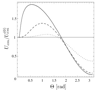
Refer to caption
Figure 2: The vdW potential of a polarizable and a magnetizable two-level atom (transition frequency ω10\omega_{10}) in the presence of an electric sphere of radius R=c/ω10R=c/\omega_{10} (ωPe/ω10=3\omega_{P_{e}}/\omega_{10}=3, ωTe/ω10=1\omega_{T_{e}}/\omega_{10}=1, γe/ω10=0.001\gamma_{e}/\omega_{10}=0.001) is shown as a function of the angular atom–atom separation Θ\Theta. The values of rA=rBr_{A}=r_{B} are 1.03​c/ω101.03\,c/\omega_{10} (solid line), 1.3​c/ω101.3\,c/\omega_{10} (dashed line), and 2​c/ω102\,c/\omega_{10} (dotted line).

Figure 3 shows the dependence of the ratio Ue​m/Ue​m(0)U_{em}/U_{em}^{(0)} on the separation distance ll between the two atoms for a configuration where the atoms are on a straight line through the center of a sphere (i.e., Θ=0\Theta=0), with the polarizable atom AA being closer to the sphere than the magnetizable atom BB. Note that in contrast to the previous configuration, in this case an electric and a magnetic sphere do not lead to equivalent results by means of duality, because the positions of the electric and magnetic atoms are not equivalent. From Fig. 3(a) it is seen that in the case of an electric sphere the interaction potential is reduced compared to its value in free space; the ratio Ue​m/Ue​m(0)U_{em}/U_{em}^{(0)} decreases with increasing ll and approaches an asymptotic limit that depends to the distance between atom AA and the sphere. In contrast, from Fig. 3(b) it is seen that in the case of a magnetic sphere the interaction potential is enhanced compared to its value in free space, and a pronounced maximum of the ratio Ue​m/Ue​m(0)U_{em}/U_{em}^{(0)} is observed. For large atom–atom distances, Ue​m/Ue​m(0)U_{em}/U_{em}^{(0)} approaches an asymptotic limit that is independent of the distance between atom AA and the sphere.

Refer to caption
Figure 3: The vdW interaction potential of two atoms with parameters as in Fig. 2 in the presence of (a) the same electric sphere as in Fig. 2, and (b) an analogous magnetic sphere is shown as a function of the atom–atom distance ll for Θ=0\Theta=0 and rB=rA+lr_{B}=r_{A}+l. The values of rAr_{A} are 1.03​c/ω101.03\,c/\omega_{10} (solid line), 1.1​c/ω101.1\,c/\omega_{10} (dashed line), 1.3​c/ω101.3\,c/\omega_{10} (dotted line).

VI Summary and concluding remarks

We have extended the framework of macroscopic QED to paramagnetic atoms by introducing a Pauli term in the atom–field interaction. We have verified the consistency of our generalized Hamiltonian by showing that it generates Maxwell’s equations and the correct equations of motion for charged particles with spin. On the basis of this Hamiltonian, we have employed leading-order perturbation theory to generalize the theory of body-assisted one- and two-atom van der Waals potentials of polarizable atoms to those that are both polarizable and magnetizable. It is seen that, with respect to each atom, the generalized potential can be considered as a superposition of contributions associated with the atomic polarizabilities and magnetizabilities. We have extended the scope of our theory to atoms that are embedded in media by implementing local-field corrections via the real-cavity model. We have found that local-field effects give rise to correction factors that depend on the permeability of the host medium for magnetizable atoms rather than the permittivity, as is the case for polarizable atoms.

We have applied the theory to the single-atom potential of an atom in the presence of a magnetoelectric half space and to the two-atom potential of atoms embedded in a bulk magnetoelectric medium or placed near a magnetoelectric sphere. The potential of a magnetizable atom in the presence of a half space has been found to be very similar to the known respective potential of a polarizable one. We have shown that a bulk medium does not change the sign of the two-atom interaction, but can lead to enhancements and reductions, whereby in the nonretarded limit the potentials of two polarizable or two magnetizable atoms is only influenced by the electric and magnetic medium properties, respectively. For the two-atom potential in the presence of a sphere, the case of two magnetizable atoms was demonstrated to be analogous to the known case of two polarizable, so we have focussed on the sphere-assisted interaction of a polarizable atom with a magnetizable one. We have obtained analytic results for a very large sphere (in which case the potential coincides with that of a half space) and a very small sphere (where the potential is analogous to the nonadditive three-atom interaction potential in free space, with the sphere taking the role of a third atom). Numerical results have been obtained for medium-sized spheres, where the sphere gives rise to enhancements and reductions of the potential, depending on the gemoetric arrangement of atoms and sphere: In particular, when the atoms are placed at equal distances from the sphere, the potential is enhanced (reduced) for small (large) separation angles between the atoms, while a linear arrangement of the atoms and the sphere (with the polarizable atom being closer to the sphere) leads to reduction (enhancement) for a electric (magnetic) sphere.

For the examples involving atoms in free space, we have explicitly verified invariance with respect to a global interchange of ε↔μ\varepsilon\leftrightarrow\mu and c2​α↔βc^{2}\alpha\leftrightarrow\beta, in agreement with the duality properties investigated in Ref. [36]. The case of two atoms in a bulk medium has further revealed that this duality invariance only holds when accounting for local-field corrections.

Acknowledgements.
This work was supported by the Alexander von Humboldt Foundation and the UK Engineering and Physical Sciences Research Council. H.S. would like to thank the ministry of Science, Research, and Technology of Iran for the financial support. S.Y.B. is grateful to G. Barton and A. Salam for discussions.

Appendix A Intermediate states and corresponding denominators in Eq. (57)

Here we list the intermediate states contributing to the vdW interaction, Eq. (57), and the corresponding energy denominators (Tab. 1).

Case |I⟩|I\rangle |I​I⟩|II\rangle |I​I​I⟩\hskip-4.30554pt|III\rangle Denominator
(11) |kA,0B⟩|1(1)⟩|k_{A},0_{B}\rangle|1_{(1)}\rangle |0A,0B⟩|1(2)1(3)⟩|0_{A},0_{B}\rangle|1_{(2)}1_{(3)}\rangle |0A,lB⟩|1(4)⟩|0_{A},l_{B}\rangle|1_{(4)}\rangle D1​a=(ωAk+ω′)​(ω′+ω)​(ωBl+ω′)D_{\mathrm{1a}}=(\omega_{A}^{k}+\omega^{\prime})(\omega^{\prime}+\omega)(\omega_{B}^{l}+\omega^{\prime}),
D1​b=(ωAk+ω′)​(ω′+ω)​(ωBl+ω)D_{1b}=(\omega_{A}^{k}+\omega^{\prime})(\omega^{\prime}+\omega)(\omega_{B}^{l}+\omega)
(22) |kA,0B⟩|1(1)⟩|k_{A},0_{B}\rangle|1_{(1)}\rangle |kA,lB⟩|{0}⟩|k_{A},l_{B}\rangle|\{0\}\rangle |0A,lB⟩|1(2)⟩|0_{A},l_{B}\rangle|1_{(2)}\rangle D2=(ωAk+ω′)​(ωAk+ωBl)​(ωBl+ω)D_{2}=(\omega_{A}^{k}+\omega^{\prime})(\omega_{A}^{k}+\omega_{B}^{l})(\omega_{B}^{l}+\omega)
(33) |kA,0B⟩|1(1)⟩|k_{A},0_{B}\rangle|1_{(1)}\rangle |kA,lB⟩|{0}⟩|k_{A},l_{B}\rangle|\{0\}\rangle |kA,0B⟩|1(2)⟩|k_{A},0_{B}\rangle|1_{(2)}\rangle D3=(ωAk+ω′)​(ωAk+ωBl)​(ωAk+ω)D_{3}=(\omega_{A}^{k}+\omega^{\prime})(\omega_{A}^{k}+\omega_{B}^{l})(\omega_{A}^{k}+\omega)
(44) |kA,0B⟩|1(1)⟩|k_{A},0_{B}\rangle|1_{(1)}\rangle |kA,lB⟩|1(2)1(3)⟩|k_{A},l_{B}\rangle|1_{(2)}1_{(3)}\rangle |0A,lB⟩|1(4)⟩|0_{A},l_{B}\rangle|1_{(4)}\rangle D4=(ωAk+ω′)​(ωAk+ωBl+ω′+ω)​(ωBl+ω′)D_{4}=(\omega_{A}^{k}+\omega^{\prime})(\omega_{A}^{k}+\omega_{B}^{l}+\omega^{\prime}+\omega)(\omega_{B}^{l}+\omega^{\prime})
(55) |kA,0B⟩|1(1)⟩|k_{A},0_{B}\rangle|1_{(1)}\rangle |kA,lB⟩|1(2)1(3)⟩|k_{A},l_{B}\rangle|1_{(2)}1_{(3)}\rangle |kA,0B⟩|1(4)⟩|k_{A},0_{B}\rangle|1_{(4)}\rangle D5=(ωAk+ω′)​(ωAk+ωBl+ω′+ω)​(ωAk+ω)D_{5}=(\omega_{A}^{k}+\omega^{\prime})(\omega_{A}^{k}+\omega_{B}^{l}+\omega^{\prime}+\omega)(\omega_{A}^{k}+\omega)
(66) |0A,lB⟩|1(1)⟩|0_{A},l_{B}\rangle|1_{(1)}\rangle |0A,0B⟩|1(2)1(3)⟩|0_{A},0_{B}\rangle|1_{(2)}1_{(3)}\rangle |kA,0B⟩|1(4)⟩|k_{A},0_{B}\rangle|1_{(4)}\rangle D6​a=(ωBl+ω′)​(ω′+ω)​(ωAk+ω′)D_{6a}=(\omega_{B}^{l}+\omega^{\prime})(\omega^{\prime}+\omega)(\omega_{A}^{k}+\omega^{\prime}),
D6​b=(ωBl+ω′)​(ω′+ω)​(ωAk+ω)D_{6b}=(\omega_{B}^{l}+\omega^{\prime})(\omega^{\prime}+\omega)(\omega_{A}^{k}+\omega)
(77) |0A,lB⟩|1(1)⟩|0_{A},l_{B}\rangle|1_{(1)}\rangle |kA,lB⟩|{0}⟩|k_{A},l_{B}\rangle|\{0\}\rangle |kA,0B⟩|1(2)⟩|k_{A},0_{B}\rangle|1_{(2)}\rangle D7=(ωBl+ω′)​(ωAk+ωBl)​(ωAk+ω)D_{7}=(\omega_{B}^{l}+\omega^{\prime})(\omega_{A}^{k}+\omega_{B}^{l})(\omega_{A}^{k}+\omega)
(88) |0A,lB⟩|1(1)⟩|0_{A},l_{B}\rangle|1_{(1)}\rangle |kA,lB⟩|{0}⟩|k_{A},l_{B}\rangle|\{0\}\rangle |0A,lB⟩|1(2)⟩|0_{A},l_{B}\rangle|1_{(2)}\rangle D8=(ωBl+ω′)​(ωAk+ωBl)​(ωBl+ω)D_{8}=(\omega_{B}^{l}+\omega^{\prime})(\omega_{A}^{k}+\omega_{B}^{l})(\omega_{B}^{l}+\omega)
(99) |0A,lB⟩|1(1)⟩|0_{A},l_{B}\rangle|1_{(1)}\rangle |kA,lB⟩|1(2)1(3)⟩|k_{A},l_{B}\rangle|1_{(2)}1_{(3)}\rangle |kA,0B⟩|1(4)⟩|k_{A},0_{B}\rangle|1_{(4)}\rangle D9=(ωBl+ω′)​(ωAk+ωBl+ω′+ω)​(ωAk+ω′)D_{9}=(\omega_{B}^{l}+\omega^{\prime})(\omega_{A}^{k}+\omega_{B}^{l}+\omega^{\prime}+\omega)(\omega_{A}^{k}+\omega^{\prime})
(1010) |0A,lB⟩|1(1)⟩|0_{A},l_{B}\rangle|1_{(1)}\rangle |kA,lB⟩|1(2)1(3)⟩|k_{A},l_{B}\rangle|1_{(2)}1_{(3)}\rangle |0A,lB⟩|1(4)⟩|0_{A},l_{B}\rangle|1_{(4)}\rangle D10=(ωBl+ω′)​(ωAk+ωBl+ω′+ω)​(ωBl+ω)D_{10}=(\omega_{B}^{l}+\omega^{\prime})(\omega_{A}^{k}+\omega_{B}^{l}+\omega^{\prime}+\omega)(\omega_{B}^{l}+\omega)
Table 1: The intermediate states contributing to the two-atom vdW interaction according to Eq. (57) together with the energy denominators, where we have used the short-hand notations |1(μ)⟩|1_{(\mu)}\rangle =\!= |1λμ​iμ​(𝒓μ,ωμ)⟩\!|\mathit{1}_{\lambda_{\mu}i_{\mu}}(\bm{r}_{\mu},\omega_{\mu})\rangle, |1(μ)​1(ν)⟩|1_{(\mu)}1_{(\nu)}\rangle =\!= |1λμ​iμ​(𝒓μ,ωμ)​1λν​iν​(𝒓ν,ων)⟩\!|\mathit{1}_{\lambda_{\mu}i_{\mu}}(\bm{r}_{\mu},\omega_{\mu})\mathit{1}_{\lambda_{\nu}i_{\nu}}(\bm{r}_{\nu},\omega_{\nu})\rangle.

Appendix B Local-field corrected tensors L and K

The local-field corrected version of the tensor L defined by Eq. (54) can be derived in complete analogy to the derivation of Eqs. (70) and (71), which was given in Refs. [19, 20]. For this purpose we recall that the first term in Eq. (71), i.e., the position-independent part of Gloc(1)​(𝒓A,𝒓A,ω)\mbox{{{{G}}}}^{(1)}_{\mathrm{loc}}(\bm{r}_{A},\bm{r}_{A},\omega), stems from the scattering Green tensor Gcav(1)​(𝒓A,𝒓A,ω)\mbox{{{{G}}}}_{\mathrm{cav}}^{(1)}(\bm{r}_{A},\bm{r}_{A},\omega) with position 𝒓A\bm{r}_{A} at the center of a small spherical cavity of radius RcR_{\mathrm{c}} which is embedded in an infinitely extended bulk material of permittivity εA\varepsilon_{A} and permeability μA\mu_{A}. The respective tensor Lcav(1)​(𝒓A,𝒓A,ω)\mbox{{{{L}}}}_{\mathrm{cav}}^{(1)}(\bm{r}_{A},\bm{r}_{A},\omega) reads [39]

Lcav(1)​(𝒓A,𝒓A,ω)=−i​ω36​π​c3​C​(ω)​I,\mbox{{{{L}}}}_{\mathrm{cav}}^{(1)}(\bm{r}_{A},\bm{r}_{A},\omega)=-\frac{\mathrm{i}\omega^{3}}{6\pi c^{3}}\,C(\omega)\mbox{{{{I}}}}, (129)

where

C⁡(ω)=−μA​h1(1)​(z)​[z0​h1(1)​(z0)]′−h1(1)​(z0)​[z​h1(1)​(z)]′μA​h1(1)​(z)​[z0​j1​(z0)]′−j1​(z0)​[z​h1(1)​(z)]′C(\omega)=\\ -\frac{\mu_{A}h_{1}^{(1)}(z)\left[z_{0}h_{1}^{(1)}(z_{0})\right]^{\prime}-h_{1}^{(1)}(z_{0})\left[zh_{1}^{(1)}(z)\right]^{\prime}}{\mu_{A}h_{1}^{(1)}(z)\left[z_{0}j_{1}(z_{0})\right]^{\prime}-j_{1}(z_{0})\left[zh_{1}^{(1)}(z)\right]^{\prime}} (130)

[z0=ω​Rc/cz_{0}=\omega R_{\mathrm{c}}/c, z=nA​z0z=n_{A}z_{0}; the primes indicate derivatives with respect to z0z_{0} and zz], with j1​(x)j_{1}(x) and h1(1)​(x)h_{1}^{(1)}(x) being the first-kind spherical Bessel and first-kind spherical Hankel functions.

The local-field correction factors multiplying G in Eqs. (70) and (71) are determined by comparing the Green tensor Gcav​(𝒓,𝒓A,ω)\mbox{{{{G}}}}_{\mathrm{cav}}(\bm{r},\bm{r}_{A},\omega) (with 𝒓A\bm{r}_{A} at the center of the cavity and 𝒓\bm{r} at an arbitrary position outside the cavity) with the bulk Green tensor Gbulk​(𝒓,𝒓A,ω)\mbox{{{{G}}}}_{\mathrm{bulk}}(\bm{r},\bm{r}_{A},\omega) of an infinite homogeneous medium without the cavity,

Gbulk​(𝒓,𝒓A,ω)=−c2​ei​k​ρ4​π​εA​ω2​ρ3​{a⁡(−i​k​ρ)​I−b⁡(−i​k​ρ)​𝒆ρ​𝒆ρ}\mbox{{{{G}}}}_{\mathrm{bulk}}(\bm{r},\bm{r}_{A},\omega)\\ =-\frac{c^{2}\mathrm{e}^{\mathrm{i}k\rho}}{4\pi\varepsilon_{A}\omega^{2}\rho^{3}}\,\left\{a(-\mathrm{i}k\rho)\mbox{{{{I}}}}-b(-\mathrm{i}k\rho)\bm{e}_{\rho}\bm{e}_{\rho}\right\} (131)

with

a⁡(x)=1+x+x2,b⁡(x)=3+3​x+x2a(x)=1+x+x^{2},\quad b(x)=3+3x+x^{2} (132)

[k=nA​ω/ck=n_{A}\omega/c, ρ=|𝒓−𝒓A|\rho=|\bm{r}-\bm{r}_{A}|, 𝒆ρ=(𝒓−𝒓A)/ρ\bm{e}_{\rho}=(\bm{r}-\bm{r}_{A})/\rho]. In the present case, the required tensor Lcav​(𝒓,𝒓A,ω)\mbox{{{{L}}}}_{\mathrm{cav}}(\bm{r},\bm{r}_{A},\omega) reads [39]

Lcav​(𝒓,𝒓A,ω)=ei​k​ρ4​π​nA2​ρ3​D​(ω)​{a⁡(−i​k​ρ)​I−b⁡(−i​k​ρ)​𝒆ρ​𝒆ρ}\mbox{{{{L}}}}_{\mathrm{cav}}(\bm{r},\bm{r}_{A},\omega)\\ =\frac{\mathrm{e}^{\mathrm{i}k\rho}}{4\pi n_{A}^{2}\rho^{3}}\,D(\omega)\left\{a(-\mathrm{i}k\rho)\mbox{{{{I}}}}-b(-\mathrm{i}k\rho)\bm{e}_{\rho}\bm{e}_{\rho}\right\} (133)

where

D⁡(ω)=\displaystyle D(\omega)=
μA​{h1(1)​(z0)​[z0​j1​(z0)]′−j1​(z0)​[z0​h1(1)​(z0)]′}μA​h1(1)​(z)​[z0​j1​(z0)]′−j1​(z0)​[z​h1(1)​(z)]′,\displaystyle\frac{\mu_{A}\left\{h_{1}^{(1)}(z_{0})\left[z_{0}j_{1}(z_{0})\right]^{\prime}-j_{1}(z_{0})\left[z_{0}h_{1}^{(1)}(z_{0})\right]^{\prime}\right\}}{\mu_{A}h_{1}^{(1)}(z)\left[z_{0}j_{1}(z_{0})\right]^{\prime}-j_{1}(z_{0})\left[zh_{1}^{(1)}(z)\right]^{\prime}}\,, (134)

and from Eq. (131), Lbulk​(𝒓,𝒓A,ω)\mbox{{{{L}}}}_{\mathrm{bulk}}(\bm{r},\bm{r}_{A},\omega) can be found to be

Lbulk​(𝒓,𝒓A,ω)=μA​ei​k​ρ4​π​ρ3​{a⁡(−i​k​ρ)​I−b⁡(−i​k​ρ)​𝒆ρ​𝒆ρ}.\mbox{{{{L}}}}_{\mathrm{bulk}}(\bm{r},\bm{r}_{A},\omega)=\frac{\mu_{A}\mathrm{e}^{\mathrm{i}k\rho}}{4\pi\rho^{3}}\,\left\{a(-\mathrm{i}k\rho)\mbox{{{{I}}}}-b(-\mathrm{i}k\rho)\bm{e}_{\rho}\bm{e}_{\rho}\right\}. (135)

Comparing Eqs. (133) and (135), we can conclude that, on using similar arguments as in Refs. [19, 20], the magnetic local-field correction factor is given by D/(μA​nA2)D/(\mu_{A}n_{A}^{2}). Combining this with Eq. (129) and following the line of reasoning of Refs. [19, 20], we expand all the terms within leading order in ω​Rc/c\omega R_{\mathrm{c}}/c to obtain the local-field corrected tensors Lloc\mbox{{{{L}}}}_{\mathrm{loc}} and Lloc(1)\mbox{{{{L}}}}_{\mathrm{loc}}^{(1)} in the form of Eqs. (74) and (75). Equation (76) follows in complete analogy.

Appendix C Green tensors L and K for a sphere

The free-space part L(0)\mbox{{{{L}}}}^{(0)} of the magnetic-magnetic tensor is the special case ε\varepsilon =\!= μ\!\mu =\!= 1\!1 of the respective bulk Green tensor (135); it obviously coincides with −(ω/c)2​G(0)-(\omega/c)^{2}\mbox{{{{G}}}}^{(0)} [which is a special case of the bulk Green tensor (131)]. According to its definition (54), the scattering part of L can be found from [39]

G(1)​(𝒓,𝒓′,ω)=i​k04​π​∑n=1∞2​n+1n⁡(n+1)​∑m=0n(2−δ0​m)​(n−m)!(n+m)!×∑p=±1[BnM(ω)𝑴n​m,p(𝒓,k0)𝑴n​m,p(𝒓′,k0)+BnN(ω)𝑵n​m,p(𝒓,k0)𝑵n​m,p(𝒓′,k0)],\mbox{{{{G}}}}^{(1)}(\bm{r},\bm{r}^{\prime},\omega)\!=\!\frac{\mathrm{i}k_{0}}{4\pi}\sum_{n=1}^{\infty}\frac{2n+1}{n(n+1)}\sum_{m=0}^{n}(2-\delta_{0m})\frac{(n-m)!}{(n+m)!}\\ \times\sum_{p=\pm 1}\left[B_{n}^{M}(\omega)\bm{M}_{nm,p}(\bm{r},k_{0})\bm{M}_{nm,p}(\bm{r}^{\prime},k_{0})\right.\\ \left.+B_{n}^{N}(\omega)\bm{N}_{nm,p}(\bm{r},k_{0})\bm{N}_{nm,p}(\bm{r}^{\prime},k_{0})\right], (136)

where BnMB_{n}^{M} and BnNB_{n}^{N} are defined by Eqs. (109) and (110), 𝑴n​m,p\bm{M}_{nm,p} and 𝑵n​m,p\bm{N}_{nm,p} are even (p=+1p=+1) and odd (p=−1p=-1) spherical wave vector functions and in spherical coordinates can be expressed in terms of spherical Hankel functions of the first kind hn(1)​(x)h^{(1)}_{n}(x) and Legendre functions Pnm​(x)P_{n}^{m}(x) as

𝑴n​m,±1​(𝒓,k)=∓msin⁡θ​hn(1)​(k​r)​Pnm​(cos⁡θ)​sincos​(m​ϕ)​𝒆θ−hn(1)​(k​r)​d​Pnm​(cos⁡θ)d​θ​cossin​(m​ϕ)​𝒆ϕ,\bm{M}_{nm,\pm 1}(\bm{r},k)=\mp\frac{m}{\sin\theta}\,h^{(1)}_{n}(kr)P_{n}^{m}(\cos\theta)\genfrac{}{}{0.0pt}{}{\sin}{\cos}(m\phi)\bm{e}_{\theta}\\ -h^{(1)}_{n}(kr)\frac{\mathrm{d}P_{n}^{m}(\cos\theta)}{\mathrm{d}\theta}\,\genfrac{}{}{0.0pt}{}{\cos}{\sin}(m\phi)\bm{e}_{\phi}, (137)
𝑵n​m,±1​(𝒓,k)=n⁡(n+1)k​r​hn(1)​(k​r)​Pnm​(cos⁡θ)​cossin​(m​ϕ)​𝒆r+1k​rd⁡[r​hn(1)​(k​r)]d​r[d​Pnm​(cos⁡θ)d​θcossin(mϕ)𝒆θ∓msin⁡θPnm(cosθ)sincos(mϕ)𝒆ϕ].\bm{N}_{nm,\pm 1}(\bm{r},k)=\frac{n(n\!+\!1)}{kr}\,h^{(1)}_{n}(kr)P_{n}^{m}(\cos\theta)\genfrac{}{}{0.0pt}{}{\cos}{\sin}(m\phi)\bm{e}_{r}\\ +\frac{1}{kr}\,\frac{\mathrm{d}[rh^{(1)}_{n}(kr)]}{\mathrm{d}r}\left[\frac{\mathrm{d}P_{n}^{m}(\cos\theta)}{\mathrm{d}\theta}\,\genfrac{}{}{0.0pt}{}{\cos}{\sin}(m\phi)\bm{e}_{\theta}\right.\\ \left.\mp\frac{m}{\sin\theta}\,P_{n}^{m}(\cos\theta)\genfrac{}{}{0.0pt}{}{\sin}{\cos}(m\phi)\bm{e}_{\phi}\right]. (138)

They are related to each other via

∇×𝑴n​m,±1​(𝒓,k)=k​𝑵n​m,±1​(𝒓,k),\displaystyle\bm{\nabla}\times\bm{M}_{nm,\pm 1}(\bm{r},k)=k\bm{N}_{nm,\pm 1}(\bm{r},k), (139)
∇×𝑵n​m,±1​(𝒓,k)=k​𝑴n​m,±1​(𝒓,k).\displaystyle\bm{\nabla}\times\bm{N}_{nm,\pm 1}(\bm{r},k)=k\bm{M}_{nm,\pm 1}(\bm{r},k). (140)

Substituting Eq. (136) into Eq. (54) and making use of the relations (139) and (140) one sees that L(1)\mbox{{{{L}}}}^{(1)} and −(ω/c)2​G(1)-(\omega/c)^{2}\mbox{{{{G}}}}^{(1)} [and consequently L and −(ω/c)2​G-(\omega/c)^{2}\mbox{{{{G}}}}] can be converted into one another by interchanging BnMB_{n}^{M} and BnNB_{n}^{N}, or equivalently interchanging ε\varepsilon and μ\mu. With this knowledge, a comparison between Eqs. (60) and (68) reveals that Um​mU_{mm} may be obtained from Ue​eU_{ee} by replacing α\alpha with β/c2\beta/c^{2} and interchanging ε↔μ\varepsilon\leftrightarrow\mu.

The scattering part of tensor K may be found by substituting Eq. (136) in (67) and making use of relations (139) and (140),

K(1)​(𝒓,𝒓′,ω)=i​k024​π​∑n=1∞2​n+1n⁡(n+1)​∑m=0n(2−δ0​m)​(n−m)!(n+m)!\displaystyle\mbox{{{{K}}}}^{(1)}(\bm{r},\bm{r}^{\prime},\omega)=\frac{\mathrm{i}k_{0}^{2}}{4\pi}\sum_{n=1}^{\infty}\frac{2n+1}{n(n+1)}\sum_{m=0}^{n}(2-\delta_{0m})\frac{(n-m)!}{(n+m)!}
×∑p=±1[BnM𝑵n​m,p(𝒓,k0)𝑴n​m,p(𝒓′,k0)\displaystyle\quad\times\sum_{p=\pm 1}\Big[B_{n}^{M}\bm{N}_{nm,p}(\bm{r},k_{0})\bm{M}_{nm,p}(\bm{r}^{\prime},k_{0})
+BnN𝑴n​m,p(𝒓,k0)𝑵n​m,p(𝒓′,k0)].\displaystyle\quad+B_{n}^{N}\bm{M}_{nm,p}(\bm{r},k_{0})\bm{N}_{nm,p}(\bm{r}^{\prime},k_{0})\Big]. (141)

Assuming, without loss of generality, that the coordinate system is chosen such that its origin coincides with the center of the sphere and the two atoms are located in the x​zxz plane as shown in Fig. 1,

𝒓A=(rA,θA,0),𝒓B=(rB,θB,π),\bm{r}_{\!A}=(r_{A},\theta_{A},0),\quad\bm{r}_{B}=(r_{B},\theta_{B},\pi), (142)

the summations over mm and pp in Eq. (141) can be performed in a way similar to Ref. [38], leading to

∑m=0n∑p=±1(2−δ0​m)​(n−m)!(n+m)!​𝑵n​m,p​(𝒓B,k0)​𝑴n​m,p​(𝒓A,k0)\displaystyle\sum_{m=0}^{n}\sum_{p=\pm 1}(2-\delta_{0m})\frac{(n\!-\!m)!}{(n\!+\!m)!}\bm{N}_{nm,p}(\bm{r}_{B},k_{0})\bm{M}_{nm,p}(\bm{r}_{A},k_{0})
=1k0​rB{n(n+1)QnsinΘPn′(γ)𝒆rB𝒆ϕA\displaystyle\quad=\frac{1}{k_{0}r_{B}}\Big\{n(n+1){Q_{n}}\sin\Theta\,P_{n}^{\prime}(\gamma)\bm{e}_{r_{B}}\bm{e}_{{\phi}_{A}}
+QnBFn(γ)𝒆θB𝒆ϕA−QnBPn′(γ)𝒆ϕB𝒆θA},\displaystyle\qquad+Q_{n}^{B}F_{n}(\gamma)\bm{e}_{{\theta}_{B}}\bm{e}_{{\phi}_{A}}-Q_{n}^{B}P_{n}^{\prime}(\gamma)\bm{e}_{{\phi}_{B}}\bm{e}_{{\theta}_{A}}\Big\}\,, (143)
∑m=0n∑p=±1(2−δ0​m)​(n−m)!(n+m)!​𝑴n​m,p​(𝒓B,k0)​𝑵n​m,p​(𝒓A,k0)\displaystyle\sum_{m=0}^{n}\sum_{p=\pm 1}(2-\delta_{0m})\frac{(n\!-\!m)!}{(n\!+\!m)!}\bm{M}_{nm,p}(\bm{r}_{B},k_{0})\bm{N}_{nm,p}(\bm{r}_{A},k_{0})
=1k0​rA{−QnAPn′(γ)𝒆θB𝒆ϕA+n(n+1)QnsinΘ\displaystyle\quad=\frac{1}{k_{0}r_{A}}\Big\{-Q_{n}^{A}P_{n}^{\prime}(\gamma)\bm{e}_{{\theta}_{B}}\bm{e}_{{\phi}_{A}}+n(n+1){Q_{n}}\sin\Theta
×Pn′(γ)𝒆ϕB𝒆rA+QnAFn(γ)𝒆ϕB𝒆θA}.\displaystyle\qquad\times\!P_{n}^{\prime}(\gamma)\bm{e}_{{\phi}_{B}}\bm{e}_{{r}_{A}}+Q_{n}^{A}F_{n}(\gamma)\bm{e}_{{\phi}_{B}}\bm{e}_{{\theta}_{A}}\Big\}\,. (144)

Combining Eqs. (141), (143) and (144) we arrive at Eq. (108) for the Green tensor.

Appendix D Limiting case of a large sphere

In the limiting case of a large sphere where the conditions (119) and (120) are met, the leading contributions to Eqs. (117) and (118) come from terms with n≫1n\gg 1 (see Ref. [32]), for which the spherical Bessel and Hankel functions can be approximated by

jn​(z)=z2(2​n+1)!!​(1−z24​n+6)j_{n}(z)=\frac{z^{2}}{(2n+1)!!}\bigg(1-\frac{z^{2}}{4n+6}\bigg) (145)

and

hn(1)​(z)=−i​(2​n−1)!!zn+1​(1+z24​n−2).h_{n}^{(1)}(z)=-i\frac{(2n-1)!!}{z^{n+1}}\bigg(1+\frac{z^{2}}{4n-2}\bigg). (146)

Hence, Eqs. (109) and (110) are approximated by

BnM​(ω)=2​i​n​(R​ω/c)2​n+1[(2​n+1)!!]2​μ⁡(ω)−1μ⁡(ω)+1B_{n}^{M}(\omega)=\frac{2\mathrm{i}n(R\omega/c)^{2n+1}}{[(2n+1)!!]^{2}}\,\frac{\mu(\omega)-1}{\mu(\omega)+1} (147)

and

BnN​(ω)=2​i​n​(R​ω/c)2​n+1[(2​n+1)!!]2​ε⁡(ω)−1ε⁡(ω)+1,B_{n}^{N}(\omega)=\frac{2\mathrm{i}n(R\omega/c)^{2n+1}}{[(2n+1)!!]^{2}}\frac{\varepsilon(\omega)-1}{\varepsilon(\omega)+1}\,, (148)

and Eqs. (111)–(113) approximately reduce to

Qn=−(cω)2​n+2​[(2​n−1)!!]2(rA​rB)n+1,\displaystyle Q_{n}=-\Bigl(\frac{c}{\omega}\Bigr)^{2n+2}\frac{[(2n-1)!!]^{2}}{(r_{A}r_{B})^{n+1}}\,, (149)
QnA=QnB=−n​Qn.\displaystyle Q_{n}^{A}=Q_{n}^{B}=-nQ_{n}. (150)

In order to illustrate the application of the approximation scheme to the tensor K(1)\mbox{{{{K}}}}^{(1)} given by Eq. (108) let us consider, for example, the component Kr​ϕ(1)K^{(1)}_{r\phi}. Making use of Eqs. (147) and (149) we find that

Kr​ϕ(1)​(𝒓B,𝒓A,ω)=X4​π​R3​μ⁡(ω)−1μ⁡(ω)+1​t2(1−2​t​g+t2)3/2K_{r\phi}^{(1)}(\bm{r}_{B},\bm{r}_{A},\omega)=\frac{X}{4\pi R^{3}}\,\frac{\mu(\omega)-1}{\mu(\omega)+1}\,\frac{t^{2}}{(1-2tg+t^{2})^{3/2}} (151)

[t=R2/(rA​rB)t=R^{2}/(r_{A}r_{B})] where the identity

∑n=1∞tn​Pn​(γ)=11−2​t​g+t2−1\sum_{n=1}^{\infty}t^{n}P_{n}(\gamma)=\frac{1}{\sqrt{1-2tg+t^{2}}}-1 (152)

has been used. Recalling condition (119), we have

tk=1−k​δA+δBR+k⁡(k+1)2​δA2+δB2R2+k2​δA​δBR2t^{k}=1-k\frac{\delta_{A}+\delta_{B}}{R}+\frac{k(k+1)}{2}\frac{\delta_{A}^{2}+\delta_{B}^{2}}{R^{2}}+k^{2}\frac{\delta_{A}\delta_{B}}{R^{2}} (153)

implying that

1−2​t​γ+t2≃Θ2+(δA+δB)2R2=l+2R2.1-2t\gamma+t^{2}\simeq\Theta^{2}+\frac{(\delta_{A}+\delta_{B})^{2}}{R^{2}}=\frac{l_{+}^{2}}{R^{2}}. (154)

Using Eq. (154) in (151) we end up with

Kr​ϕ(1)​(𝒓B,𝒓A,ω)=X4​π​l+3​μ⁡(ω)−1μ⁡(ω)+1.K_{r\phi}^{(1)}(\bm{r}_{B},\bm{r}_{A},\omega)=\frac{X}{4\pi l_{+}^{3}}\frac{\mu(\omega)-1}{\mu(\omega)+1}. (155)

The other components of K(1)\mbox{{{{K}}}}^{(1)} can be evaluated in a similar way. Substituting the resulting expressions for K(1)\mbox{{{{K}}}}^{(1)} into Eqs. (106) and (107), and summing them in accordance with Eq. (105) leads to Eq. (121).

References

  • [1] A. Salam, Int. Rev. Phys. Chem. 27, 405 (2008).
  • [2] F. London, Z. Phys. 63, 245 (1930).
  • [3] H. B. G. Casimir, Proc. K. Ned. Akad. Wet. 51, 793 (1948).
  • [4] B. M. Axilrod and E. Teller, J. Chem. Phys. 11, 299 (1943).
  • [5] B. M. Axilrod, J. Chem. Phys. 17, 1349 (1949).
  • [6] M. R. Aub and S. Zienau, Proc. R. Soc. London, Ser. A 257, 464 (1960).
  • [7] E. A. Power and T. Thirunamachandran, Proc. R. Soc. London, Ser. A 401, 267 (1985).
  • [8] E. A. Power and T. Thirunamachandran, Phys. Rev. A 50, 3929 (1994).
  • [9] G. Feinberg and J. Sucher, J. Chem. Phys. 48, 3333 (1968).
  • [10] T. H. Boyer, Phys. Rev. 180, 19 (1969).
  • [11] G. Feinberg and J. Sucher, Phys. Rev. A 2, 2395 (1970).
  • [12] E. Lubkin, Phys. Rev. A 4, 416 (1971).
  • [13] M. Babiker and G. Barton, Proc. R. Soc. London, Ser. A 326, 255 (1972).
  • [14] A. D. McLachlan, Mol. Phys. 7, 381 (1964).
  • [15] J. Mahanty and B. W. Ninham, J. Phys. A: Math. Gen. 6, 1140 (1973).
  • [16] H. Safari, S. Y. Buhmann, D.-G. Welsch, and D. T. Ho, Phys. Rev. A 74, 042101 (2006).
  • [17] S. Y. Buhmann, H. Safari, D.-G. Welsch, and D. T. Ho, Open Syst. Inf. Dyn. 13, 427 (2006).
  • [18] L. Onsager, J. Am. Chem. Soc. 58, 1486 (1936).
  • [19] D. T. Ho, S. Y. Buhmann, and D.-G. Welsch, Phys. Rev. A 74, 023803 (2006).
  • [20] A. Sambale, S. Y. Buhmann, D.-G. Welsch, and M. S. Tomaš, Phys. Rev. A 75, 042109 (2007).
  • [21] S. Spagnolo, D. A. R. Dalvit, and P. W. Milloni, Physical Review A 75, 052117 (2007).
  • [22] L. Knöll, S. Scheel, and D.-G. Welsch, in Coherence and Statistics of Photons and Atoms, edited by J. Peřina (Wiley, New York, 2001), p. 1.
  • [23] S. Y. Buhmann, D. T. Ho, L. Knöll, and D.-G. Welsch, Phys. Rev. A 70, 52117 (2004).
  • [24] S. Y. Buhmann and D.-G. Welsch, Prog. Quantum Electron. 31, 51 (2007).
  • [25] C. Baxter, M. Babiker, and R. Loudon, Phys. Rev. A 47, 1278 (1993).
  • [26] D. P. Craig and T. Thirunamachandran, Molecular Quantum Electrodynamics (Dover, New York, 1998).
  • [27] D. T. Ho, S. Y. Buhmann, L. Knöll, D.-G. Welsch, S. Scheel, and J. Kästel, Phys. Rev. A 68, 43816 (2003).
  • [28] E. A. Power and S. Zienau, Phil. Trans. R. Soc. London Ser. A 251, 427 (1959).
  • [29] R. G. Woolley, Proc. R. Soc. London, Ser. A 321, 557 (1971).
  • [30] A. A. Kyasov and G. V. Dedkov, Surf. Sci. 463, 11 (2001).
  • [31] H. B. G. Casimir and D. Polder, Phys. Rev. 73, 360 (1948).
  • [32] S. Y. Buhmann, D. T. Ho, T. Kampf, and D.-G. Welsch, Eur. Phys. J. D 35, 15 (2005a).
  • [33] J. K. Jenkins, A. Salam, and T. Thirunamachandran, Phys. Rev. A 50, 4767 (1994).
  • [34] A. Salam, Int. J. Quantum Chem. 78, 437 (2000a).
  • [35] A. Salam, J. Phys. B: At. Mol. Opt. Phys. 33, 2181 (2000b).
  • [36] S. Y. Buhmann and S. Scheel, arXiv:0809.3975 (2008).
  • [37] S. Y. Buhmann, T. Kampf, and D.-G. Welsch, Phys. Rev. A 72, 032112 (2005b).
  • [38] H. Safari, D.-G. Welsch, S. Y. Buhmann, and D. T. Ho, Phys. Rev. A 77, 053824 (2008).
  • [39] L.-W. Li, P.-S. Kooi, M.-S. Leong, and T.-S. Yeo, IEEE Trans. Microwave Theory Tech. 42, 2302 (1994).