Characterizing graphs with convex and connected Cayley configuration spaces
Abstract
We define and study exact, efficient representations of realization spaces Euclidean Distance Constraint Systems (EDCS), which include Linkages and Frameworks. These are graphs with distance assignments on the edges (frameworks) or graphs with distance interval assignments on the edges. Each representation corresponds to a choice of non-edge (squared) distances or Cayley parameters. The set of realizable distance assignments to the chosen parameters yields a parametrized Cayley configuration space. Our notion of efficiency is based on the convexity and connectedness of the Cayley configuration space, as well as algebraic complexity of sampling realizations, i.e., sampling the Cayley configuration space and obtaining a realization from the sample (parametrized) configuration. Significantly, we give purely graph-theoretic, forbidden minor characterizations for 2D and 3D EDCS that capture (i) the class of graphs that always admit efficient Cayley configuration spaces and (ii) the possible choices of representation parameters that yield efficient Cayley configuration spaces for a given graph. We show that the easy direction of the 3D characterization extends to arbitrary dimension and is related to the concept of -realizability of graphs. Our results automatically yield efficient algorithms for obtaining exact descriptions of the Cayley configuration spaces and for sampling realizations, without missing extreme or boundary realizations. In addition, our results are tight: we show counterexamples to obvious extensions.
This is the first step in a systematic and graded program of combinatorial characterizations of efficient Cayley configuration spaces. We discuss several future theoretical and applied research directions.
In particular, the results presented here are the first to completely characterize EDCS that have connected, convex and efficient Cayley configuration spaces, based on precise and formal measures of efficiency. It should be noted that our results do not rely on genericity of the EDCS. Some of our proofs employ an unusual interplay of (a) classical analytic results related to positive semi-definiteness of Euclidean distance matrices, with (b) recent forbidden minor characterizations and algorithms related to -realizability of graphs. We further introduce a novel type of restricted edge contraction or reduction to a graph minor, a “trick” that we anticipate will be useful in other situations.
Keywords: Underconstrained Geometric Constraint System, Mechanism, Cayley configuration space, Combinatorial rigidity, Linkage, Framework, Graph Minor, Graph Characterization, Distance geometry, Convex, Semidefinite and Linear programming, Algebraic Complexity.
1 Introduction
A Euclidean Distance Constraint System (EDCS) is a graph together with an assignment of distances , or distance intervals to the edges . A -dimensional realization is the assignment of points in to the vertices in such that the distance equality (resp. inequality) constraints are satisfied: , respectively . Note the EDCS with distance equality constraints, , is also called a linkage and was originally referred to as a framework in combinatorial rigidity terminology; more recently a framework includes a specific realization , and the distance assignment is read off from .
We seek efficient representations of the realization space of an EDCS. We define a representation to be (i) a choice of parameter set, specifically a choice of a set of non-edges of , and (ii) a set of possible distance values that the non-edges can take while ensuring existence of at least one -dimensional realization for the augmented EDCS: . In the presence of inequalities, the Cayley configuration space is denoted and the augmented EDCS is: . Here refers to a graph . In other words, in this manuscript, our representations are in Cayley parameters or non-edge distances: the set (resp. ) is the projection onto the Cayley parameters in , of the Cayley-Menger semi-algebraic set with fixed (resp. ) [6, 29, 8]. This is also the set of dimensional Euclidean distance matrix completions of the partial distance matrix specified by [1].
We refer to the representation (resp. ) as the Cayley configuration space of the EDCS (resp. ) on the parameter set of non-edges of .
Note. For ease of exposition, from now on EDCS will generally refer to distance equality constraints only. We will indicate with explicit remarks when a theorem is applicable to EDCS with distance inequality constraints as well.
The PhD thesis [11] formulates the concept of efficient Cayley configuration space description for EDCS by emphasizing the exact choice of parameters used to represent the realization space. This sets the stage for a mostly combinatorial, and complexity-graded program of investigation. An initial sketch of this program was presented in [12]; a comprehensive list of theoretical results and applications to date can be found in the PhD thesis [11].
1.1 Organization
In Sections 2 and 2.1 we motivate and give a brief background for the overall program of investigation. The questions of interest and contributions of this manuscript are listed in Section 3. Their novelty and technical significance are outlined in Section 4 together with related work. Formal results and proofs are presented in Section 5. We conclude with suggestions for future work in Section 6.
2 Motivation
Describing and sampling the realization space of an EDCS is a difficult problem that arises in many classical areas of mathematics and theoretical computer science and has a wide variety of applications in computer aided design for mechanical engineering, robotics and molecular modeling. Especially for underconstrained or independent and not rigid EDCS whose realizations have one or more degrees of freedom of motion, progress on this problem has been very limited.
Existing methods for sampling EDCS realization spaces often use Cartesian representations, factoring out the Euclidean group by arbitrarily “pinning” or “grounding” some of the points’ coordinate values. Even when the methods use “internal” representation parameters such as Cayley parameters (non-edges) or angles between unconstrained objects, the choice of these parameters is adhoc. While Euclidean motions may be automatically factored out in the resulting parametrized Cayley configuration space, for most such parameter choices, the Cayley configuration space is still a topologically complex semi-algebraic set, sometimes of reduced measure in high dimensions.


After the representation parameters are chosen, the method of sampling the Cayley configuration space often reduces to “take a uniform grid sampling and throw away sample configurations that do not satisfy given constraints.” Since even Cayley configuration spaces of full measure (representation using lowest possible number of parameters or dimensions) often have complex boundaries, potentially with cusps and large holes, this type of sampling is likely to miss extreme and boundary configurations and is moreover computationally inefficient. To deal with this, numerical, iterative methods are generally used when the constraints are equalities, and in the case of inequalities, probabilistic “roadmaps” and other general collision avoidance methods are used. They are approximate methods. If the Cayley configuration space is relatively low dimensional, then initial sampling is used to provide an approximate and refinable representation of the Cayley configuration space, using traditional approximation theory methods such as splines or computational geometry representations, for example, based on Voronoi diagrams. Thereafter this approximate representation is used to guide more refined sampling. All of these are approximate methods that do not leverage exact descriptions of the Cayley configuration space.
Two related problems additionally occur in NMR molecular structure determination and wireless sensor network localization: completing a partially specified Euclidean Distance Matrix in a given dimension; and finding a Euclidean Distance Matrix in a given dimension that closely approximates a given Metric Matrix (representing pairwise distances in a metric space) [5, 10]. The latter problem also arises in the study of algorithms for low distortion embedding of metric spaces into Euclidean spaces of fixed dimension [2]. Both of these can be viewed as searching over a Cayley configuration space of an EDCS. But the common methods for these problems are different from those used for exploring Cayley configuration spaces. One reason for this is that usually only one realization is usually sought, which optimizes some appropriately chosen function; the goal is not sampling or description of the entire Cayley configuration space. Common methods for these problems are: (i) either use semi-definite programming, since Euclidean Distance Matrices in a specified dimension are directly related to Gram matrices which are positive semidefinite matrices of a specified rank; (ii) or iteratively enforce the Cayley-Menger determinantal conditions that characterize Euclidean Distance Matrices in a specified dimension.
2.1 Exact, efficient Cayley configuration spaces
Motivated by these applications, our emphasis is on exact, efficient description of the Cayley configuration space of underconstrained or independent and not rigid EDCS. (i) An exact algebraic description guarantees that boundary and extreme configurations are not missed during sampling, which is important for many applications. (ii) An efficient description (i.e, low dimensional, full measure, convex, using few polynomial or even linear inequalities, whose coefficients are obtained efficiently from the given EDCS) is important for tractability of the sampling algorithm.
Efficiency refers to several factors. We list four efficiency factors that are relevant to this manuscript. The first factor is the sampling complexity: given the EDCS , (i) the complexity of computing (ia) the set of Cayley parameters or non-edges and (ib) the description of the Cayley configuration space as a semi-algebraic set, which includes the algebraic complexity of the coefficients in the polynomial inequalities that describe the semi-algebraic set, and (ii) the descriptive algebraic complexity, i.e., number, terms, degree etc of the polynomial inequalities that describe the semi-algebraic set. These together determine the complexity of sampling or walking through configurations in .
Concerning (ia), it is important to note that most choices of Cayley parameters (non-edges) to represent the realization space of give inefficient descriptions of the resulting parametrized Cayley configuration space (see for example Figures 1,2). Hence we place a strong emphasis is on a systematic, combinatorial choice of the Cayley parameters that guarantee a Cayley configuration space with all the efficiency requirements listed here. Further, we are interested in combinatorially characterizing for which graphs such a choice even exists.
The second efficiency factor is the realization complexity. Note that the price we pay for insisting on exact and efficient Cayley configuration spaces is that the map from the traditional Cartesian realization space to the parametrized Cayley configuration space is many-one. I.e, each parametrized or Cayley configuration could correspond to many (but at least one) Cartesian realizations.
However, we circumvent this difficulty by defining and studying realization complexity as one of the requirements on efficient Cayley configuration spaces i.e., we take into account that the realization step typically follows the sampling step, and ensure that one or all of the corresponding Cartesian realizations can be obtained efficiently from a parametrized sample configuration.
A third efficiency factor is generic completeness, i.e, we would like (a) each configuration in our parametrized configuration space to generically correspond to at most finitely many Cartesian realizations and (b) we would like the Cayley configuration space to be of full measure, and in particular, they use at most as many parameters or dimensions as the internal degrees of freedom of . Specifically (a) means is rigid and (b) means is not overconstrained, i.e, it is independent. This generic completeness means that the graph is wellconstrained i.e., minimally rigid.
Note. In this paper, unless otherwise specified, we always assume that Cayley configuration spaces have full measure.
A fourth and fifth important efficiency factors are topological and geometric complexity for example, number of connected components, and convexity. Convexity and connectedness are natural properties to study since they facilitate convex programming and other efficient methods for sampling. Another crucial reason for studying convexity is that results (such as those presented here) about convex configuration spaces readily generalize from Euclidean distance equality constraint systems (e.g. frameworks) to Euclidean distance inequality constraint systems (e.g. tensegrities and partially specified Euclidean Distance Matrices with intervals as entries).
2.2 Combinatorial Characterization
Combinatorial characterizations of generic properties of EDCS are the cornerstone of combinatorial rigidity theory. In practice they crucial for tractable and efficient geometric constraint solving, since they are used to analyze and decompose the underlying algebraic system. So far such characterizations have been used primarily for broad classifications into well- over- under- constrained, detecting dependent constraints in overconstrained systems and finding completions for underconstrained systems. Such combinatorial characterizations have been missing in the finer classification of underconstrained systems according to the efficiency or complexity of their Cayley configuration space. Our emphasis in this respect is the surprising fact that there is a clean combinatorial characterization at all for the algebraic complexity of configuration spaces. This however is a necessary step in efficiently decomposing and analyzing underconstrained systems.
3 Questions and Contributions
Next we give 4 natural questions concerning efficient configuration spaces and the contribution of this manuscript towards answering them.
3.1 Question 1: Graphs with connected, convex, linear polytope 2D Cayley configuration spaces
We are interested in characterizing for which there is a set of non-edges such that for all distance assignments (resp. intervals ), the -dimensional Cayley configuration space (resp. ), is convex or connected or is a linear polytope. Furthemore, given in this characterized class, we would like to characterize the corresponding sets of non-edges. These are exactly the parameter choices that yield efficient Cayley configuration spaces.
Note. Here the phrase linear polytope refers to aspect (ib) of the sampling complexity defined in Section 2: the coefficients of the linear inequalties that define the bounding hyperplanes of the polytope are simple linear combinations of the given determined by and . Contrast this with a polytope for which the coefficients of the bounding linear inequalities are the solution of an arbitrary polynomial system determined by and .
- (1)
In Theorem 5.10, we give an exact characterization of the class of graphs all of whose corresponding EDCS admit a 2D (generically complete), linear polytope Cayley configuration space. The theorem also shows that the characterization remains unchanged if the Cayley configuration space is merely required to be convex, and further if it is merely required to be connected.
- (2)
For a graph in the above class, in Theorem 5.11 we give an exact combinatorial characterization of the choices of Cayley parameters (non-edges) that ensure a (generically complete), linear polytope Cayley configuration space.
- (3)
Both above results rely on key Theorem 5.1 (in turn based on Theorem 5.2) that characterizes a graph along with a non-edge such that for all distance assignments , the 2D Cayley configuration space , is a single interval. We additionally show in Observation 5.9 that this result is tight in that the obvious analog of this result fails in 3D.
- (4)
Observation 5.12 shows that while the forward direction of Theorem 5.10, Theorem 5.11, and Theorem 5.1 for pure distance constraints holds directly for interval constraints , the reverse direction fails. However, in Theorem 5.13, we give an exact characterization of the class of graphs all of whose corresponding EDCS admit a 2D (generically complete), linear polytope, convex or connected Cayley configuration space.
We note that the forward direction of the above theorems (that the graph-theoretic property always admits a convex, connected, linear polytope Cayley configuration space) is straightforward. It is the reverse direction that is surprising and the proof requires a new type of restricted edge-contraction reduction to a graph minor (see Section 4).
3.2 Question 2: Graphs with universally inherent, connected and convex configuration spaces
One can view Contributions (2) and (3) above as characterizing pairs such that always admits a connected or convex Cayley configuration space on . Sometimes, it is more convenient to instead characterize the graphs In particular, we say that a graph always admits an inherent connected or convex Cayley configuration space, if there exists a partition of the edges of into so that the graph always admits a connected or convex Cayley configuration space on . In other words, for all distance assignments (resp. intervals ) for the the graph , the -dimensional Cayley configuration space (resp. ), is connected or convex. We additionally consider the following strong property. We say that a graph always admits universally inherent connected or convex Cayley configuration spaces, if for every partition of the edges of into , the graph always admits a connected or convex Cayley configuration space on . We are interested in combinatorially characterizing graphs that always admit universally inherent connected or convex Cayley configuration spaces.
- (5)
A graph is -realizable if for every for which the EDCS has a Euclidean realization in any dimension, it also has a realization in . This useful notion of -realizability was introduced by [3, 4], which also showed a forbidden minor characterization of such graphs for . For any dimension , we show in Theorem 5.15 that the class of -realizable graphs always admit universally inherent connected Cayley configuration spaces, that are in fact convex over squared Cayley parameters. We refer to those as convex squared Cayley configuration spaces. This result holds also when the corresponding EDCS use distance intervals.
- (6)
Theorem 5.16 shows the reverse direction of (5) for 3D, and thus shows that 3-realizable graphs are exactly the ones that always admit universally inherent connected and convex 3D squared Cayley configuration spaces, also when the corresponding EDCS use distance intervals. Thus, by [3, 4], this class also has forbidden minor characterization. In Observation 5.9, we observe that both Theorem 5.15 and Theorems 5.16 are weak statements for 2D – much stronger statements follow directly from (2) above. For example, it follows from (2) that if a graph is not 2-realizable, then there is a natural component of the graph that does not even admit an inherent connected Cayley configuration space description, leave alone a universally inherent one.
3.3 Question 3: Efficiently recognizing graphs with connected and convex configuration spaces
- (7)
Both characterizations in Contributions (1) and (6) (Theorems 5.11 and 5.16) directly point to efficient, existing algorithms that recognize whether a given graph always admits (universally inherent) connected, convex, (generically complete), linear polytope 2D and 3D (squared) Cayley configuration spaces. For example, a recent algorithm for recognizing 3-realizable graphs [36] was given based on a characterization of such graphs in [3].
3.4 Question 4: Sampling and Realization complexities
The practical use of the contributions (1)-(6) above becomes apparent when we answer the following question. Given an EDCS (resp. ) where is in one of the classes characterized in contributions (1) to (6), what is the complexity of computing (i) an appropriate set of Cayley parameters or non-edges (ii) the exact description of (resp. ) as a semi-algebraic set (iii) a cartesian realization of a given parametrized configuration in . Here (i) and (ii) determine the sampling complexity and (iii) determines realization complexity.
- (8)
For 2D, Theorem 5.10 and Theorem 5.11 shows that the time complexities for (i), (ii) and (iii) are linear. For 3D, our result in Theorem 5.16 only pertains to universally inherent Cayley configuration spaces, and we only have a weak analog of Theorem 5.11, hence Question 4(i) only marginally applies. We observe that a result from [36] gives a weak answer for question (i) and an time complexity for (iii). The complexity for (ii) is an open problem and is discussed in Section 6. However, by employing Contribution (5) (Theorem 5.16), the complexity of obtaining one configuration is seen to be polynomial (in contrast to obtaining a full description of the Cayley configuration space as a semi-algebraic set).
4 Novelty and Related Work
- •
The study of the cartesian realizations of plane linkages or EDCS with distance equality constraints has a long history [25]: over a century ago, Kempe showed that any plane algebraic curve can be traced by a point in the realizations of a linkage. Furthermore, there are extensive studies of the topology of the configuration space of, for example, polygonal linkages parametrized by Cayley parameters, see for example [14].
However, to the best of our knowledge, ours is the first combinatorial or graph-theoretic forbidden minors characterization of geometric and topological complexity such as convexity, and connectedness of Cayley configuration spaces in Cayley parameters even for the plane, and certainly for 3D.
Conceptually, the results on global rigidity [20, 21] (resp. globally linked pairs [22]) are related, since they combinatorially characterize when the Cayley configuration space on all (resp. specific) Cayley parameters (non-edges) is a single point. However, these characterizations hold only generically [9, 17] as is customary for many combinatorial properties related to rigidity. In contrast, we note that our characterizations apply to all EDCS’ (frameworks) and not just generic frameworks. This is a crucial distinction that is needed to reconcile apparent discrepancies of the two types of results, as we elaborate in Section 6.1.2 together with a conjecture concerning the modification of our characterization for generic frameworks.
Moreover, in Section 6.1.6 we point out that the class of EDCS with convex (squared) Cayley configuration spaces is much larger than in our characterization, when the distances associated with the edges of the EDCS are known to be special. Furthermore, in Sections 6.1.4 we point out that the class of EDCS that admit connected 3D Cayley configuration spaces - that are not necessarily universally inherent - is also much larger than in our characterization. Both these observations have computational chemistry applications as pointed out in Sections 6.2.2 and 6.2.3.
Our results additionally yield a combinatorial characterization of sampling complexity. This incorporates the complexity of (i) obtaining the chosen set of parameters and (ii) the algebraic complexity of obtaining the description of the Cayley configuration space from the given graph. This in turn includes the descriptive complexity of the Cayley configuration space as a semi-algebraic set, such as the number and degree of the polynomials. The characterizations moreover incorporate realization complexity, i.e, the complexity of obtaining a realization from a parametrized configuration.
To the best of our knowledge, the only results of a similar flavor are: the result of [31] that shows the equivalence of Tree- or Triangle- decomposability [30] and Quadratic or Radical realizability for planar graphs; and the result characterizing the sampling complexity of 1-dof Henneberg-1 graphs [13].
- •
Concerning the use of Cayley parameters or non-edges for parametrizing a generically complete Cayley configuration space: [34] as well as [24, 37] study how to obtain “completions” of underconstrained graphs , i.e, a set of non-edges whose addition makes minimally rigid or well-constrained. Both are motivated by realization complexity of underconstrained EDCS: i.e, efficiently obtaining a realization given the parameters values of a configuration, i.e, once the distance values of the completion edges in are given. In particular [24] also guarantees that the completion ensures Tree- or Triangle- decomposability, thereby ensuring low realization complexity. However, they do not even attempt to address the question of how to find realizable distance values for the completion edges. Nor do they concern themselves with the geometric, topological or algebraic complexity of the set of distance values that these completion non-edges can take, nor the complexity of obtaining a description of this Cayley configuration space, given the EDCS and the non-edges , nor a combinatorial characterization of graphs for which this sampling complexity is low. The latter factors however are crucial for tractably analyzing and decomposing underconstrained systems and for sampling their Cayley configuration spaces in order to obtain the corresponding realizations. The problem has generally been considered too messy, and barring effective heuristics for certain cases, for example in [28], there has been no systematic, formal program to study this problem.
- •
Some of the proofs (e.g. Theorem 5.15) employ an unusual interplay of (i) classical analytic results related to (squared) Euclidean distance matrices, such as positive semi-definiteness that date back to [33], with (ii) recent graph-theroretic characterizations [3, 4] related to -realizability. This further permits us to directly apply a recent result about efficient realization of 3-realizable EDCS [36].
- •
5 Theorems
5.1 Basics
We start with basic definitions and facts. Take two graphs and that both contain a complete graph on vertices, , as a proper subgraph. For any matching of the vertices of the two ’s, by identifying the matched pairs, we can get a new graph . We call this procedure a -sum of and [3]. A graph is a k-tree if it is a -sum of ’s. Given a graph, we can run the inverse operations of -sum to get a set of -sum components. If we can not run the inverse operations of -sum for a component, we say that component is a minimal (-sum) component. Given a non-edge , a minimal -sum component containing is a minimal subgraph that is both a -sum component and contains the vertices of . We emphasize that the phrase does not refer to a -sum component that is minimal and happens to contain .
A graph is a partial k-tree if it is a subgraph of a -tree. Please refer to Figure 3 for 2-trees and partial 2-trees and Figure 4 for 2-sum and 2-sum component. It is not hard to see that partial 2-trees are exactly the 2-realizable graphs. While partial 3-trees are in fact 3-realizable, the class of 3-realizable graphs include non partial 3-trees as well.
In [3, 4] a useful forbidden-minor characterization of such graphs is given. A graph has a graph as a minor if there is a vertex induced subgraph of that can be reduced to via edge removals and edge contractions (coalescing or identifying the 2 vertices of an edge). It is not hard to see that partial 2-trees are exactly the graphs that avoid minors.
Next we give basic 2D combinatorial rigidity definitions based on Laman’s theorem [26]. For 3D, no combinatorial definitions exist. For the corresponding algebraic definitions, please see for example [19] (combinatorial rigidity terminology) [15] [34] (geometric constraint solving terminology).
In 2D, a graph is wellconstrained or minimally rigid if it satisfies the Laman conditions [26]; i.e., and for all subgraphs of ; is underconstrained or independent and not rigid if we have and for all subgraphs . A graph is overconstrained or dependent if there is a subgraph with . is welloverconstrained or rigid if there exists a subset of its edges such that the graph is wellconstrained or minimally rigid. A graph is flexible if it is not rigid.
5.2 Graphs with connected, convex, linear polytope 2D Cayley configuration space
We are interested in characterizing graphs that always admit a convex, connected or linear polytope Cayley configuration space; i.e, graphs for which there is a set of non-edges such that for all distance assignments (resp. intervals ), the -dimensional Cayley configuration space (resp. ), is convex or connected or is a linear polytope.
Furthemore, given in this characterized class, we would like to characterize the corresponding sets of non-edges. These are exactly the parameter choices that yield well-behaved Cayley configuration spaces.


Figure 3 gives an example graph that admits a connected, convex and linear polytope 2D Cayley configuration space on the specified non-edges; and viceversa, in Figure 5, we provide an example in which the graph does not admit such a Cayley configuration space on any non-edge. The graph characterization of Theorem 5.1 can be easily verified for both examples.
5.2.1 Graphs and their “single-interval” non-edges
The next theorem characterizes a graph along with a non-edge such that the Cayley configuration space of on is always a single interval.
Theorem 5.1
Given a graph and a non-edge , the Cayley configuration space is a single interval for all if and only if all the minimal 2-sum components of that contain are partial 2-trees.

Structure of Proof: To prove one (harder) direction of Theorem 5.1, we need the following purely graph-theoretic theorem and the following Lemma 5.5. The other (easy) direction follows from Lemma 5.8 which is in turn proven gradually using Lemma 5.6 and Lemma 5.7.
Theorem 5.2


Remark 5.3
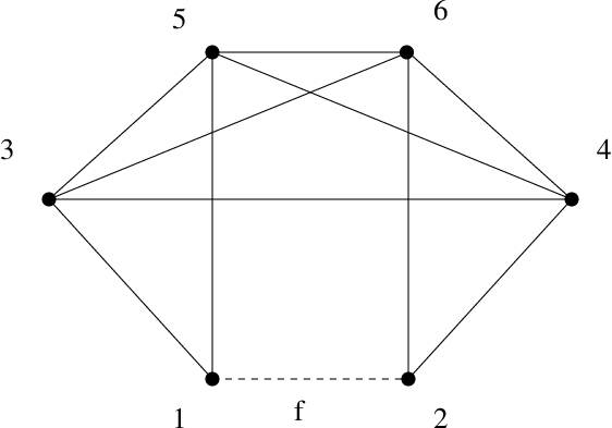
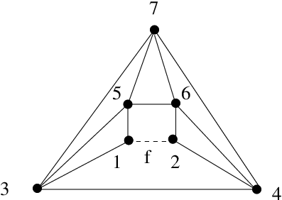
The two base cases Figure 6 and Figure 7 are based on . Based on the fact that partial 2-trees do not have minors and properties of 2-sum, we can prove one direction of Theorem 5.2. For the other direction the existence of a minor alone is insufficient. We require a special type of pure edge-contraction reduction without edge removals, which additionally preserve selected non-edges: i.e, prevent them from becoming edges or from collapsing to a single vertex.
Proof [Theorem 5.2] We first prove that cannot be reduced to Figure 6 or Figure 7 by edge contractions if all the minimal 2-Sum components of containing are partial 2-trees. Because partial 2-trees do not have minors, and since exists as a minor in both Figure 6 and Figure 7, we cannot reduce to either of the two base cases by edge contractions (no edge removals). In fact, in case there exists a 2-sum component that does not contain , our proof will not change since edge contractions either preserve 2-sum relationship or transform a 2-sum to a 1-sum.
We prove the other direction by induction on the number of vertices of . The statement is true for the 2 base cases. Assume the statement is true for ; we prove it for .

First, we remove and to get a set of connected components (Figure 8). We use to denote the subgraph of which is induced by vertices of together with and , where . Note that each is a 2-sum component of . Without loss of generality, we assume is one of these 2-sum components of but not a partial 2-tree.
Case . If , the number of vertices of is . Hence by the induction hypothesis, we can reduce to the one of the two base cases by edge contractions. Now we just contract all the edges of when and the resulting graph falls into the base case in Figure 7.
Case . In this case, there is only one minimal 2-sum component containing and it is not a partial 2-tree. If is not , the number of vertices of is . By the induction hypothesis we can reduce to one of the two base cases. By contracting all the edges of which are not in , we can reduce to one of the base cases. (Note that a 1-sum is a special case of a 2-sum.) If, on the other hand, , then it is a minimal 2-sum component containing and it is not a partial 2-tree. There are 2 subcases based on , the maximum number of disjoint paths between and , the vertices of .

[Subcase ] we can find a vertex, say , that separates and , that is, we can split the graph into two subgraphs and such that , ; and share only vertex , and all the edges of are either in or (refer to Figure 9 for this case). Since is a minimal 2-sum component containing both and , both and have to be non-edges. In addition, at least one of and is not a partial 2-tree, otherwise will also be a partial 2-tree. Without loss of generality, suppose is not a partial 2-tree. By the induction hypothesis, we can reduce to one of the two base cases. By contracting all the edges in we can also reduce to one of the two base cases ( is identified with ).

[Subcase ] Take two disjoint paths and . We can contract to and to (Figure 10). If we further remove ,, and , we get new connected components. Then we contract all the edges inside these new connected components such that each of them becomes a single vertex that we denote by . Before we contract paths and , if we remove and , the remaining graph is still connected(), so at least one of is connected to both and .
Now we contract edges as follows (refer to Figure 10).
- 1.
if connects to both and , we can identify with by edge contraction;
- 2.
if connects to only and (not to or ), we leave it unchanged;
- 3.
if connects to only one of ,, and , we identify it with the corresponding vertex in ,, and ;
- 4.
if connects to ,, , we can identify with ;
- 5.
if connects to ,, , we can identify with .
That covers all the cases and completes the proof of the induction step.
Theorem 5.2 gives us the following independently interesting corollary.
Corollary 5.4
Given graph and a non-edge , we can reduce to one of the base cases in Figure 6 or Figure 7 by a sequence of edge contractions provided the following hold.
- 1.
itself is the minimal 2-sum component containing .
- 2.
For any vertex other than and , either is 2 and is adjacent to both and , or is at least three.
- 3.
At least one vertex other than and has degree of three or more.
Proof The proof is by contradiction. Suppose (1), (2), (3) hold but can not be reduced to either of the two base cases. Then by Theorem 5.2, all the minimal 2-sum components of the graph containing and are partial 2-trees. Note that at least one vertex other than and has degree of three or more. We consider the 2-sum component containing . Note also that has more than 3 vertices, and within , since (2) holds, there can be no vertices other than and that have degree of two or less. By (2), any other vertex of degree two or less would be adjacent to both and and would form its own 2-sum components.
Now note that in any 2-tree with more than 3 vertices, there exist two non-adjacent vertices which both have degree of two, so in any partial 2-tree with more than 3 vertices, there should also exist two non-adjacent vertices which both have degree of at most two. This contradicts the fact that and (which are adjacent) are the only vertices in that have degree of two or less.
Using Corollary 5.4, we see that the graph in Figure 5 can be reduced to one of the two base cases no matter which non-edge we choose.
Proof Follows from reflection across edge . Let , , , and all be 1 and and be 2, we can easily check that possible values of are or , so is not connected.
As noted earlier, Theorem 5.2 and Lemma 5.5 have proved the difficult direction for Theorem 5.1. The following lemmas prove the easy direction.
Lemma 5.6
If is the 2-sum of , then for any , has a realization if and only if each , ( restricted to the edges in ) has a realization.
Proof [Lemma 5.6]
Simply hinge all the 2-sum components’ realizations along the 2-sum edges to get a realization of , with any one of two reflection choices across the 2-sum edge. The other direction is immediate.
Lemma 5.7
Take a graph with 2-sum components , and a non-edge set that is entirely contained in an arbitrary one of the , say . Then for any , either if all the ’s are non-empty, i.e., the EDCS have at least 1 realization; or otherwise, is empty.
Proof
Directly follows from Lemma 5.6.
Lemma 5.8
- (a)
If a graph has a 2-sum component that is an underconstrained partial 2-tree, then there exists a nonempty non-edge set entirely in such that for any , is a linear polytope. Moreover, there is such a set such that is generically complete for .
- (b)
If a graph is an underconstrained partial 2-tree, then for any nonempty non-edge set that preserves as a partial 2-tree, and for all , is a linear polytope.
Proof
For proving (a), we will construct a nonempty set of non-edges in and show that the projection on is a linear polytope for all .
Note that is an underconstrained partial 2-tree, so we can find a nonempty subset of non-edges of by adding which we get a 2-tree. We let be this nonempty set. Note that such an is a completion for , i.e., makes minimally rigid. Hence we know that is of full-measure and generically complete, proving the last sentence of the theorem.
To get the linear polytope, note that a 2-tree can be written as the 2-sum of triangles. For example, let , and denote the length of the three edges of the triangle , then the triangle inequalities are , and .
Thus, for all , is a linear polytope. Now since is entirely in , Lemma 5.7 applies and for all , or is empty. Thus, for all , is also a linear polytope.
For proving (b): for any underconstrained partial 2-tree , we can find a nonempty non-edge set that makes a 2-tree; and we showed that for any , is a generically complete linear polytope 2D Cayley configuration space. Take any nonempty subset of of such a - these are exactly the subsets of non-edges whose addition would preserve the partial 2-tree property of . Then is the projection of on and since the latter is a linear polytope, the former is a linear polytope as well.
Proof [Theorem 5.1] The proof of one (harder) direction follows directly from Theorem 5.2 and the Lemma 5.5. Specifically, to pick a distance assignment for that yields a disconnected Cayley configuration space on , we set all the contracted edges during the procedure of Theorem 5.2 to 0. The uncontracted edges are now mapped by the reduction to edges of one of the base cases. Lemma 5.5 tells us how to choose those distance values to ensure disconnectedness of the Cayley configuration space on . The other (easy) direction is immediate from Lemma 5.8.
Next we show that Theorem 5.1 is tight in that neither of the two straightforward extensions to 3D hold.
Observation 5.9
There exists a partial 3-tree(resp. 3-realizable graph) and non-edge such that is not a partial 3-tree(resp. 3-realizable graph) and yet is always connected.
5.2.2 Graphs with generically complete, linear polytope Cayley configuration spaces
In Theorem 5.10, we give an exact characterization of the class of graphs , all of whose corresponding EDCS admit a 2D (generically complete), linear polytope Cayley configuration space. The theorem also shows that the characterization remains unchanged if the Cayley configuration space is merely required to be convex, and further if it is merely required to be connected.
Theorem 5.10
(a)For a graph , the following four statements are equivalent:
- 1.
There exists a non-empty set of non-edges such that for all is connected;
- 2.
There exists a non-empty set of non-edges such that for all , is convex;
- 3.
There exists a non-empty set of non-edges such that for all is a linear polytope.
- 4.
has a 2-sum component that is an underconstrained partial 2-tree.
(b)An underconstrained graph always admits a generically complete linear polytope, connected or convex Cayley configuration space if and only if every underconstrained 2-sum component of is a partial 2-tree.
Proof For (a), we will prove the cycle . We proved in Lemma 5.8. A linear polytope is convex, so follows. Convexity implies connectedness, so follows. Theorem 5.1 and the proof of Lemma 5.8 proves , therefore, we proved as well.
For one direction of (b): if every underconstrained 2-sum component of is an underconstrained partial 2-tree, then by Lemma 5.8, always admits a generically complete linear polytope, connected or convex Cayley configuration space. The reverse direction of (b) follows from (a) (1,2,3 4): if always admits a generically complete linear polytope, connected or convex Cayley configuration space, has at least one 2-sum component which is an underconstrained partial 2-tree.
5.2.3 Full characterization of Cayley parameters that yield a linear polytope 2D Cayley configuration space
The following theorem is a refined version of Theorem 5.10.
Theorem 5.11
Given a graph and non-empty set of non-edges , the 2D Cayley configuration space is a linear polytope, connected or convex for all if and only if all the minimal 2-Sum components of containing any subset of are partial 2-Trees. Furthermore, the Cayley configuration space is generically complete if and only if all the underconstrained minimal 2-sum components of are partial 2-trees and all the minimal 2-sum components of containing are 2-trees.
5.2.4 Characterization of EDCS with distance intervals
We have characterized graphs and sets of non-edges where the Cayley configuration space is connected, convex and a linear polytope for all . We can extend the results for distance interval constraints. The next observation and theorem show that while one direction of the above results extends to interval constraints, the other direction fails in the current form. This motivates a modified characterization theorem.
Observation 5.12
There exists a graph and non-edge such that all the minimal 2-Sum components of containing are partial 2-trees and yet we can find an interval distance constraint such that is not linear polytope convex, or connected.
Proof Refer to Figure 13. Denote the graph shown in Figure 13 (a) by and the graph shown in Figure 13 (a) by . Denote non-edge by in both Figure 13 (a) and (b). Clearly, has 3 minimal 2-sum components: the subgraph induced by , the subgraph induced by and the subgraph induced by . The first two minimal 2-sum components both contain and both are partial 2-trees. The third one (the subgraph induced by ) is not a partial 2-tree but does not contain . By Theorem 5.1, for all distance , the Cayley configuration space is connected. Similarly, has 2 minimal 2-sum components: the subgraph induced by , and the subgraph induced by . Both two minimal 2-sum components contain . The first one is not a partial 2-tree and the second one (the subgraph induced by ) is not a partial 2-tree. By Theorem 5.1, we can find distance such that the Cayley configuration space is not connected. If we allow an interval distance constraint on edge in , we would have an equivalent distance constraint sytem as .

Now we give a characterization theorem for distance interval constraints.
Theorem 5.13
Given a connected graph and a nonempty set of non-edges , the 2D Cayley configuration space is linear polytope, convex or connected for all if and only if every minimal 2-Sum component of a specific subdivision of that contains any subset of is a partial 2-tree. We construct the subdivision of by replacing each edge by a path of length 2 by introducing a new vertex
Proof For a given interval constraint , we can choose and such that the distance constraints on the subdivision, namely and together impose the original distance interval constraint on the edge . Then by Theorem 5.11, is a linear polytope, connected or convex for all if and only if all the minimal 2-Sum components of containing a subset of are partial 2-Trees.
5.3 Graphs with universally inherent, convex, squared Cayley configuration spaces
5.3.1 -realizability implies convex, squared Cayley configuration spaces
We will prove in Theorem 5.15 that -realizable graphs admit universally inherent, connected (resp. convex) -dimensional (resp. squared) Cayley configuration spaces. Before that, we first show in Lemma 5.14 that convexity of squared Cayley configuration spaces implies connectedness of the Cayley configuration space.
Note. All the results in the section apply to both distance constraints as well as distance interval constraints . In order to avoid writing: “for all (resp. ) the (resp. squared) Cayley configuration space (resp. ) is connected (resp. convex)” we instead just say “ always admits a connected (resp. convex) (resp. squared) Cayley configuration space”.
Lemma 5.14
If a graph always admits universally inherent, convex, -dimensional squared Cayley configuration spaces, then it also always admits universally inherent, connected, -dimensional configuration spaces.
Proof For a non-edge set of , denote by the Cayley configuration space: has a realization in . The map is continuous and the inverse map is well-defined and continuous over the positive reals. Now the convexity of implies its connectedness, that by the above-mentioned continuity implies the connectedness of .
Now we are ready to give the theorem and the proof.
Theorem 5.15
If a graph is -realizable, it admits universally inherent, connected (resp. convex), -dimensional (resp. squared) Cayley configuration spaces.
Proof By Lemma 5.14, we only need to prove a -realizable graph admits universally inherent, convex, squared Cayley configuration spaces.
A matrix is a Euclidean square distance matrix (EDM) if for some such that . A classical result [33] that follows from positive semidefiniteness of Gram matrices is that the set of all EDM’s is a convex cone (note that , and hence the rank of these matrices is not fixed). The projection of this cone on any set of pairs is also convex. By the definition of -realizability of a graph , with , this projection is exactly the set of all squared distance assignments to the pairs in for which has a realization in . We denote this . Since convexity is preserved by both sections and projections, the section of this projection - obtained by fixing to be over - is also convex, for all . This section is exactly the Cayley configuration space of the graph over its nonedge set . Hence this is a convex squared Cayley configuration space. Note that this holds for any partition of the edge set of the -realizable graph . Hence always admits universally inherent, convex, squared Cayley configuration spaces.
5.3.2 When does universally inherent, connected configuration
space imply
-realizability?
Theorem 5.16
Let . Then the following are equivalent for a graph .
- 1.
is -realizable.
- 2.
always admits universally inherent, connected, -dimensional Cayley configuration spaces.
- 3.
always admits universally inherent, convex, -dimensional squared Cayley configuration spaces.
Remark 5.17
The above theorem is a weak statement for . For example, since the class of 2-realizable graphs is exactly the partial 2-trees, Theorem 5.11 shows that if a graph is not 2-realizable, then it has a minimal 2-sum component that is not 2-realizable (not a partial 2-tree). And this component does not admit any inherent Cayley configuration space, let alone universally inherent ones. In other words, in this non 2-realizable minimal 2-sum component , on a vertex set for every partition of edges into , the Cayley configuration space of graph is disconnected. For , on the other hand, no such strong statement holds as shown in the counterexample of Observation 5.9. To show the above theorem, we merely show that if a graph is not 3-realizable, then there exists a partition of the edges of into , such that the configuration space of the graph is disconnected.
Structure of Proof. The proof of the above theorem requires several lemmas. The idea of the proof is as follows. Lemma 5.14 proves (3)(2), and Theorem 5.15 proves (1)(3) for all dimensions . Based on the above remark, we restrict ourselves to , and just prove (2)(1).
For any non-3-realizable graph , we find a partition of as where is the graph and find a distance assignment such that the Cayley configuration space is disconnected. Here and is a single non-edge of , so this is a 1-parameter Cayley configuration space and we show that it has 2 isolated points. To do this, we start from the following theorem.
Theorem 5.18 (Connelly and Sloughter [3, 4])
A graph is 3-realizable if and only if it does not have or as minors.
Given the existence of one of these 2 minors, as in Theorem 5.2, we show how to pick from the graph and its non-edges such that by a restricted reduction that uses only edge contractions (no edge removals) and preserving the non-edges , we can reduce the graph to a or that is missing exactly one edge, namely , on to which all the non-edges in have been mapped by the reduction. Finally, we obtain using Lemma 5.21 the distance assignment for by setting the distances for the contracted edges to 0; and, similar to Lemma 5.5 we pick distance assignments for the un-contracted edges in such a way that the two base cases do not have connected 3D Cayley configuration spaces on .
We will use the following simple fact.
Fact 5.19
If a graph has a complete graph , as a minor, then can be reduced to by edge contraction alone (and removal of isolated vertices if necessary), without edge removals.
We also need the following independently interesting theorem which strengthens the forbidden-minor theorem of Theorem 5.18.
Theorem 5.20
If a graph is not 3-realizable, it can be reduced to or by edge contractions alone (no edge removals).
Proof
If a graph is not 3-realizable, it has a or minor by Theorem 5.18. If a graph has a minor, use Fact 5.19, it can be reduced to by edge contractions alone, so we only need to prove the case that has a as minor. If has a as minor, by definition of minor we can get a by first contracting some edges, then removing some edges, and finally removing some isolated vertices. Follow this reduction path but stop after edge contractions, and denote the new graph by . Denote the subgraph of by .
Now we will show we can either get or a by edge-contractions and removing some isolated vertices if necessary. The strategy is straight forward: successively contract one edge at a time, whose two vertices are not both in until we cannot continue. After removing any possible isolated vertices, the remaining graph has exactly 6 vertices(the same as ) and we denoted this graph by . We know that is a subgraph of . Now we use a simple observation that by adding one or more edges to , we can get a by edge contractions alone, thus can be reduced to or by edge contractions alone.
For proving the next lemma, we give an appropriate distance assignment to and to show they do not admit universally inherent, connected Cayley configuration spaces.

Lemma 5.21
Neither nor always admit universally inherent, connected, 3D Cayley configuration spaces.
Proof To prove the Lemma for (resp. ), we take one edge as and prove that we can find a distance assignment for graph (resp. ) such that (resp. ) has more than one interval.
For case, we take to be and assign the same distances to all the edges in . If we fix tetrahedron , then can either be coincident with or is the reflection of about plane . Since is not in the plane , so in the latter case, is not zero. In the former case, is zero. These two values are all the possible values of , so we have proved that is not connected.
For case (Figure 14), we choose edge as . We choose a distance assignment so that the following conditions are satisfied: , , , and will let .
Because , , and are collinear and the four vertices , , and are coplanar. Because and , will be equal to and . Thus, the location of will be uniquely determined by the normal tetrahedron if we assume that, without loss of generality, is above plane . Now has two possible locations, either or the reflection of about plane . We denote the former location as while the latter as . For the case when is coincident with , will be . For the other case, by the triangle inequality in , we have . Now and are normal tetrahedrons and is different from in this case, so is not in the plane . Therefore, can not be collinear with and , so . Thus has two disconnected values and we have proved that projection is not connected.
Now we are ready to prove Theorem 5.16.
Proof [Theorem 5.16] By Theorem 5.15, a 3-realizable graph admits universally inherent connected, convex, 3D squared Cayley configuration spaces, so we only need to prove the reverse direction. If is not 3-realizable, by Theorem 5.20, we can get a or by edge contractions alone.
As mentioned before, find a partition of the edge set of into that defines a subgraph and a non-edge set for . Then find a distance assignment for such that is disconnected.
Since can be reduced to or by edge contractions alone, we pick an edge from the corresponding minor and denote it . We choose to be all the edges that were identified with by the reduction. For the distance assignment to the edges of , we will use a similar method as in the proof of Theorem 5.1. Lemma 5.21 gives a distance assignment for and that ensures that the Cayley configuration space on the edge is disconnected. Set the distances of each uncontracted edge during the reduction of to the distance assignment of the edge in or that was identified with. Set the distances of all the contracted edges of to be 0. This ensures that is disconnected.
5.4 Efficiently recognizing graphs with connected and convex Cayley configuration spaces
Theorems 5.10 and 5.16 characterize when a given graph always admits (universally inherent) connected, convex, (generically complete), linear polytope 2D and 3D (squared) Cayley configuration spaces. Based on these theorems, we give efficient algorithms to recognize these properties.
Theorem 5.22
Given a graph , both for the case of distance constraints as well as for distance interval constraints, there are linear time algorithms to recognize:
- 1.
whether there is a non-empty set of non-edges such that always admits a connected (convex, linear polytope) 2D Cayley configuration space on .
- 2.
under the assumption that is not over-constrained, whether there is a set of non-edges such that always admits a connected (convex, linear polytope) generically complete 2D Cayley configuration space on .
- 3.
whether always admits universally inherent, connected (resp. convex), -dimensional (resp. squared) Cayley configuration spaces, for .
Proof For (1), first note that a linear time algorithm decomposes the input graph to 2-sum components. By Theorem 5.10, there is a non-empty set of non-edges such that always admits a connected (convex, linear polytope) 2D Cayley configuration space on , for the case of distance constraints if and only if has a 2-sum component that is an underconstrained partial 2-tree. Thus, we only need to check whether there exists a 2-sum component that is an underconstrained partial 2-tree. Checking if a graph is a partial 2-tree can be done in linear time. Since partial 2-trees are always independent, i.e, they cannot be overconstrained, they are underconstrained exactly if the number of edges is at most twice the number of vertices minus 3 (the Laman count). Thus the entire check can be done in linear time.
Under the assumption that does not have overconstrained subgraphs, the algorithm for (2) is essentially the same as (1). By Theorem 5.1, check whether all underconstrained 2-sum components are partial 2-trees. Find any set of nonedges that complete them into 2-trees, which are automatically wellconstrained or minimally rigid. This guarantees a generically complete Cayley configuration space on . The assumption that has no overconstrained subgraphs is necessary for the above algorithm to work: for example, suppose the input graph is a 2-sum of two graphs and where is an underconstrained partial 2-tree while is not a partial 2-tree. There is a complete set of non-edges for such that always admits a generically complete, connected, convex and linear polytope 2D Cayley configuration space. However, in order to check whether yields a generically complete Cayley configuration space for all of , we have to ensure that is rigid. If no overconstrained subgraphs exist, then this can be determined by a Laman count for in linear time. Otherwise, we would need to detect the presence of overconstrained subgraphs. In general, network flow based algorithms [16, 34], and even more efficient pebble game algorithms [23] [27] exist for this check.
For (1) and (2) in the case of distance interval constraints, Theorem 5.13 permits us to perform the same checks and in linear time on a subdivision of that is at most 2 times the size of the edge set of .
For (3), by Theorem 5.16, which applies to both distance and distance interval constraints, we only need to check whether a graph is 2-realizable( partial 2-tree) and 3-realizable. The former is straightforward. Based on [3], a linear algorithm is proposed in [36] to check whether a graph is 3-realizable.
5.5 Practical use: Sampling and Realization Complexities
Theorem 5.22 gives us the algorithms to find a set of non-edges that ensure (generically complete), connected, convex, linear polytope Cayley configuration spaces. They prove Points (1), (2), (3) of the Theorem below. For practical use we need to further get the exact description of (resp. ) (sampling complexity) and also a cartesian realization of a given parametrized configuration in (resp. ) (realization complexity).
Theorem 5.23
Given an EDCS , or , where the corresponding graphs are recognized by the algorithms of Theorem 5.22, there are linear time algorithms that:
- 1.
output a set of non-edges such that always admits a (generically complete) connected (convex, linear polytope) 2D Cayley configuration space on .
- 2.
under assumption is not overconstrained, output a set of non-edges such that always admits a connected (convex, linear polytope) generically complete 2D Cayley configuration space on .
- 3.
output a maximal set of non-edges such that the graph always admits universally inherent, connected 2D or 3D Cayley configuration spaces.
- 4.
For in all of the above items, output a corresponding description of a linear polytope 2D Cayley configuration space (resp. ) provided it is known to be nonempty; additionally, if one realization is known, then given any input element in the 2D Cayley configuration space, output its corresponding realization in .
Given an EDCS , or , there is a polynomial time algorithm that
- (5)
for the in Item 3, outputs one configuration in the configuration space (resp. ); additionally, when given an input element of this 3D Cayley configuration space, outputs a realization .
Proof As pointed out earlier, the proof of Theorem 5.22 also proves (1),(2). For (3), for 2D, we simply output a set of non-edges so that is a complete 2-tree. For 3D, using a characterization theorem of 3-realizable graphs , by [3, 4], and an algorithm of [36], we can output a maximal set of edges such that such that remains 3-realizable. This gives the desired graph by Theorem 5.15.
For (4), for the case of distance constraints alone, the proof of Lemma 5.8 gives a linear time algorithm to find the description of the linear polytope 2D configuration space on as a system of linear inequalities. For the case of distance interval constraints, the same algorithm can be applied to the subdivision graph given by Theorem 5.13 to get the description. The assumption that the Cayley configuration space is non-empty is required because by Lemma 5.7, the Cayley configuration space of would be empty if any of EDCS corresponding to a non-partial-2-tree 2-sum components of has no realization; and determining if a general EDCS has a realization is an NP-hard problem.
For the second statement in (4): take (resp. ) to be any of the 2-sum components of (resp. ) that contain a subset of . When an element, of a Cayley configuration space of such an EDCS is given, if (resp. ) are complete 2-trees, the corresponding EDCS (resp. ) are Quadratically or Radically realizable. I.e., they can be realized by a straightforward ruler-and-compass construction involving a sequence of solutions of univariate quadratics (intersection of circles). On the other hand, if (resp. ) are not complete 2-trees, they can be made complete 2-trees by additional edges , for which can be extended consistently, i.e., in such a way that has a realization whenever has a realization. The realizations of the remaining 2-sum components (that do not contain any subset of ), in particular those that may not be partial 2-trees, can be read off from the one given realization . As shown in Lemma 5.6, realizations of the different 2-sum components do not interfere with each other: i.e., the realizations of the various 2-sum components can be hinged together along the 2-sum edges to get the realization of the entire graph. Again, the realization is required because finding a realization for the EDCS of a 2-sum component that is a general graph (not necessarily a partial 2-tree) is a hard problem (the decision version is NP-hard [32]).
For (5), simply using the definition of 3-realizable graphs, we can obtain one point of the Cayley configuration space of on the given as follows. Use the positive semidefiniteness of the Euclidean distance matrix cone to complete the distances or distance intervals (for the edges of as given by ) into a full Euclidean distance matrix for some dimension . This could be much larger than 3. Since we know that the given satisfies the property that is also 3-realizable, by the definition of 3-realizability, if we pick the distances for from the completed matrix, then it would be guaranteed to be a point in the Cayley configuration space of on .
6 Conclusions and Conjectures
Our results give a practically meaningful, and mathematically robust definition of exact and efficient Cayley configuration spaces of underconstrained Euclidean Distance Constraint Systems (equalities and inequalities), based on various efficiency factors including complexity of sampling and realization. We have taken the first step in a systematic and graded program sketched in [12] and laid out in [11] - for the combinatorial characterizations of efficient Cayley configuration spaces. In particular, the results presented here characterize graphs and their Cayley parameters that yield (squared) Cayley configuration spaces that are connected, convex, linear polytopes, and efficient algorithms for sampling realizations.
6.1 Theoretical Directions and Conjectures
6.1.1 Is -realizability equivalent to universally inherent, connected -dimensional Cayley configuration spaces?
Our first conjecture is the reverse direction of Theorem 5.15.
Conjecture 6.1
For any dimension , a graph is -realizable if and only if it always admits universally inherent, connected (resp. convex) -dimensional squared Cayley configuration spaces.
6.1.2 The roles of Genericity and Independence

Our results characterize (for the case of distance equalities and frameworks) Cayley configuration space properties that hold for all distance assignments , and are hence incorrect if we require the properties to hold only in generic situations. For example, Figure 15 shows a generically globally rigid graph : the generic 2D Cayley configuration space of this graph on the non-edge is a single point. However, by our Theorem 5.1, since a minimal 2-sum component containing is not 2-realizable, the Cayley configuration space on is disconnected. The apparent discrepancy arises because the proof of the Lemma 5.2 uses non-generic specializations of the edge distances in the process of reduction to a minor which then shows that the Cayley configuration space on is disconnected for that , which is sufficient to prove the statement of Lemma 5.2 and Theorem 5.1. We believe, however that both these results still hold under a genericity assumption, provided the graph is not overconstrained (independent, in rigidity terminology) and the non-edge is not globally-linked.
Conjecture 6.2
Given a graph that is not generically over-constrained and a non-edge , the Cayley configuration space is a single interval for all generic (i.e., for that admit a 2D generic realization of ), if and only if all the minimal 2-sum components containing are 2-realizable and (partial 2-trees).
6.1.3 Sampling complexity for 3D
Note that while we know from Theorem 5.16 that 3-realizable graphs always admit universally inherent, convex, 3D squared Cayley configuration spaces, we do not yet know an efficient algorithm to determine their description. This is necessary to determine the sampling complexity. This is in stark contrast to the linear time algorithm for obtaining such descriptions in the case of 2D (Theorem 5.11).
One straightforward algorithm for obtaining the description of the Cayley configuration space as a semi-algebraic set is to start with the Cayley-Menger [8, 6, 29] determinantal equalities and inequalities for Euclidean distance matrices in -dimensions. These are polynomial relationships between all the Cayley parameters, including those in , and those in . Eliminating those in , and specifying the values for the parameters in in to be leaves polynomial equalities and inequalities in the Cayley parameters in . This yields the required description of the Cayley configuration space as a semi-algebraic set.
Viewed in this manner, it appears remarkable that in 2D, for the graphs and non-edge sets satisfying the conditions of Theorem 5.11, this above-described elimination leaves only the triangle inequalities relating the Cayley parameters in and (note that these were part of the original Cayley-Menger set of inequalities) and hence we get a linear polytope description of . Note however that we did not use such an elimination for our proof!. Our proof that these triangle inequalities give a description of was through a more direct route: we determined for what configuration for the Cayley parameters in we could construct a 2D realization for the augmented EDCS .
We would like to show a similar result in 3D either by using elimination or using Euclidean distance matrix completion for fixed rank [1, 5] by a more direct route of determining when 3D realizations can be constructed.
Conjecture 6.3
Let be a 3-realizable graph on vertex set . Take any partition of the edge set of into , and consider the graph and any EDCS . Then there is a time algorithm to write down the description of the Cayley configuration space as a semi-algebraic set of low degree (say, no more than 4).
In this context, note that there is also room to improve the sampling complexity and obtain more refined descriptions even for 2D Cayley configuration spaces of graphs satisfying the conditions of Theorem 5.11. For this purpose, it makes sense to study complete 2-trees on a set of vertices . In particular, after partitioning the edges of into and eliminating all except the set of Cayley parameters in we obtain a system of linear inequalities in those parameters, which we call the 2D admissible distance polytope of . I.e, it specifies the distance assignments for which has a 2D realization. Note that this is the projection of the 2D admissible distance polytope for , onto the parameters in . Furthermore, the Cayley configuration space is a section or a fibre of this polytope. In [7] we study the detailed topology of these polytopes, towards extending similar studies of polytopes corresponding to the simpler class of polygonal linkages parametrized by Cayley parameters, see for example [14].
6.1.4 Characterizing all parameters that ensure connected, Cayley squared configuration spaces for 3D
It would be desirable to extend Theorem 5.1 (and hence Theorems 5.10 and 5.11) to a characterization of parameter choices for 3D connected Cayley configuration spaces. As pointed out in Observation 5.9 the obvious analog of this result fails in 3D. Partial results supporting the following conjecture have been reported in [11]. Note that partial 3-trees are a large proper subclass of 3-realizable graphs.
Conjecture 6.4
Given graph that is a partial 3-tree and non-edge
- •
if has no or minor, then has a connected 3D Cayley configuration space on ;
- •
if has a or minor then has a connected 3D Cayley configuration space on if and only if the 2 vertices of must be identified in order to get a or minor in .
6.1.5 1-dof 2D mechanisms and 2D Cayley configuration spaces with 2 connected components
There are 2 possible directions to move beyond the connected, convex, linear-polytope 2D configuration spaces.
The first is to study the Cayley configuration spaces of 1-dof graphs that just fail to satisfy the requirements of Theorem 5.2. A first step in this direction has been taken by [13], see also [11], and future research suggestions along that direction has been presented there.
The second direction is to study which graphs always admit Cayley configuration spaces with 2 or fewer connected components? Partial results in this direction have been reported in [11], specifically towards characterizing graphs and non-edges such that the 2D Cayley configuration space of on has no more than 2 intervals.
6.1.6 Stronger results for special distance assignments
Our characterizations apply to all distance assignments or distance intervals . This places strong restrictions on the characterized classes of graphs with efficient Cayley configuration spaces. However, if one assumes special distance assignments, well-behaved Cayley configuration spaces may exist for much larger classes of graphs. For example, consider the 2D 2-direction grid, which is not a partial 2-tree. However, under the restriction of unit-distance edges, [11] shows that such an EDCS has a Cayley configuration space that is a convex polytope, in fact a rectilinear box. Moreover, for such an EDCS, [11] gives a complete characterization of Cayley parameters (non-edges) on which the Cayley configuration space is convex. It would be desirable to obtain similar results for 3D, due to potential applications in Section 6.2 below.
6.2 Practical Implications for Mechanical CAD and Computational Chemistry
6.2.1 Realization space and motion exploration for CAD mechanisms
Representation of realization spaces of underconstrained systems is a long-standing issue in the development of constraint solvers underlying mechanical CAD systems. Our characterizations and algorithms for obtaining efficient configuration spaces and sampling realizations would be useful to incorporate into commercial constraint solvers. However, they need to be implemented in combination with other practical user- or designer-driven functionalities.
In addition to sampling realizations, our program of comprehensive study of possible parameter choices is useful for geometrically meaningful exploration of the motions of underconstrained systems, or mechanisms. Current (infinitesimal) motion representation reduces to a basis choice for the motion space obtained from the rigidity matrix for a particular realization . Obvious basis choices lead to an erratic exploration of the motion space, often amplifying spurious “globally” coupled motions or “allosteric” effects instead of systematically first exploring “locally” coupled motions to the extreme or boundary configurations.
Intuitively, our theorems give choices of Cayley parameters that ensure convex or otherwise well-behaved Cayley configuration spaces and hence each standard method of walking these spaces invests a geometric meaning to the corresponding systematic motion exploration, especially since Cayley parameters are particularly suited to representing internal motion. Furthermore any standard method of walking a convex Cayley configuration space would fully explore “locally” coupled motions before systematically progressing to less local ones. It would be desirable to state and prove a formal statement to this effect.
6.2.2 Sampling realization space for helix packing
Helix packing is a well-studied computational chemistry problem since helices are prevalent in many biomolecules. One part of the problem can be viewed as sampling the realization space of an EDCS (including distance inequalities) that correspond to steric or collision avoidance and other constraints. Current methods use inexact representations of realization spaces and “generate and test” algorithms for sampling them. As a result they are inefficient and moreover lack any guarantee that all boundary and extreme realizations have been explored.
Partial results [11] (see Section 6.1.4) give parameter choices that ensure connected and convex, 3D squared Cayley configuration spaces even for non 3-realizable graphs. By the characterization proved here, these are clearly not universally inherent. Based on these Cayley parameter choices, an algorithm for exact description and efficient, systematic sampling of the helix packing configuration spaces (especially the boundaries and extreme points) is given in [35].
6.2.3 Limit properties and Sampling of realization spaces for Zeolite sequences
Zeolites are naturally occuring materials whose structure can be described as “corner sharing regular tetrahedra.” The corresponding EDCS sequences involve only distance equalities and are obtained from progressively larger pieces of an infinite lattice structure with uniform boundary conditions. The goal is to sample the realization spaces of these Zeolite EDCS sequences, with a view to understanding their properties in the limit.
Since the Zeolite EDCS have special distance assignments, as pointed out in Section 6.1.6, they have efficient Cayley configuration spaces even if the corresponding graphs may not satisfy the requirements of the characterization theorems presented in this manuscript. Using similar results such as a characterization of Cayley configuration spaces of 2D unit-distance grid graphs mentioned in Section 6.1.6, [11] presents partial results on the configuration spaces of a class of Zeolite sequences.
subsection*Acknowledgements Special thanks to the participants of the Barbados (McGill) workshops on Rigidity and molecular modeling organized by Ileana Streinu and Mike Thorpe in 2006 and 2007. Those workshops helped in discovering several of the applications listed in Section 6.2.
References
- [1] A. Y. Alfakih, A. Khandani and H. Wolkowicz. Solving Euclidean Distance Matrix Completion Problems via Semidefinite Programming. Comput. Optim. Appl., 12:13–30, 1999.
- [2] M. Bădoiu, K. Dhamdhere, A. Gupta, Y. Rabinovich, H. Räcke, R. Ravi and A. Sidiropoulos. Approximation algorithms for low-distortion embeddings into low-dimensional spaces. SODA ’05: Proceedings of the sixteenth annual ACM-SIAM symposium on Discrete algorithms, page 119–128, 2005.
- [3] Maria Belk (Sloughter) and Robert Connelly. Realizability of Graphs. Discrete & Computational Geometry, 37(2):125–137, 2007
- [4] Maria Belk. Realizability of Graphs in Three Dimensions. Discrete & Computational Geometry, 37(2):139–162, 2007
- [5] Pratik Biswas, Tzu-Chen Lian, Ta-Chung Wang and Yinyu Ye. Semidefinite programming based algorithms for sensor network localization. ACM Trans. Sen. Netw., 2(2):188–220, 2006.
- [6] L.M. Blumenthal. Theory and Applications of Distance Geometry. Oxford University, 1953.
- [7] C. Borcea, M. Sitharam and I. Streinu. The admissible distance polytope of partial 2-trees. In preparation.
- [8] A. Cayley. A theorem in the geometry of position. Cambridge mathematical Journal., II:267–271, 1841.
- [9] Robert Connelly. Generic global rigidity. Discrete & Computational Geometry, 33(4):549–563, 2005
- [10] G.M. Crippen and T.F. Havel. Distance Geometry and Molecular Conformation. Chemometrics series, 15, Taunton, Somerset, England: Research Studies Press, 1998.
- [11] H. Gao. Geometric Under-Constraints. Ph.D. thesis, University of Florida, Gainesville, FL, 2008.
- [12] H. Gao, and M. Sitharam. Combinatorial Classification of 2D Underconstrained Sytems. Proceedings of the Seventh Asian Symposium on Computer Mathematics (ASCM 2005), Sung-il. Pae. and Hyungju. Park., Eds., 2005, pp. 118–127.
- [13] H. Gao and M. Sitharam. Characterizing 1-Dof Henneberg-I graphs with efficient configuration spaces. arXiv:0810.1997 [cs.CG].
- [14] Jean-Claude Hausman. Geometric descriptions of polygon and chain spaces Topology and Robotics, Amer. Math. Soc., vol. 438, pages 47–57, 2007.
- [15] Christoph M. Hoffmann, Andrew Lomonosov and Meera Sitharam. Decomposition of geometric constraints systems, part i: performance measures. Journal of Symbolic Computation, 31(4), 2001.
- [16] Christoph M. Hoffmann, Andrew Lomonosov and Meera Sitharam, Decomposition of geometric constraints systems, part ii: new algorithms. Journal of Symbolic Computation, 31(4), 2001.
- [17] Steven J. Gortler, Alexander D. Healy and Dylan P. Thurston. Characterizing Generic Global Rigidity. arXiv:0710.0926v3 [math.MG].
- [18] T. Gower. Weblog: http://gowers.wordpress.com/2007/09/11/what-might-an-expository-mathematical-wiki-be-like/.
- [19] J. E. Graver, B. Servatius, and H. Servatius. Combinatorial Rigidity. Graduate Studies in Math., AMS, 1993.
- [20] Bruce Hendrickson. Conditions for unique graph realizations. SIAM J. Comput., 21(1):65-84, 1992.
- [21] Bill Jackson and Tibor Jordán, Connected rigidity matroids and unique realizations of graphs. J. Comb. Theory, Ser. B, 94(1):1-29, 2005.
- [22] Bill Jackson, Tibor Jordán and Zoltan Szabadka. Globally Linked Pairs of Vertices in Equivalent Realizations of Graphs. Discrete & Computational Geometry, 35(3):493-512, 2006.
- [23] Donald J. Jacobs and Bruce Hendrickson. An algorithm for two dimensional rigidity percolation: The pebble game. J. Computational Physics, 137:346-365, 1997.
- [24] Robert Joan-Arinyo, Antoni Soto-Riera, S. Vila-Marta and Josep Vilaplana-Pasto. Transforming an under-constrained geometric constraint problem into a well-constrained one. Symposium on Solid Modeling and Applications 2003, pages 33–44, 2003.
- [25] Alfred Bray Kempe. On a general method of describing plane curves of the th degree by linkwork. Proc. London Math Soc. vol. 7, pages 213–216, 1876.
- [26] G. Laman. On graphs and rigidity of plane skeletal structures. J. Engrg. Math., vol. 4, page 331–340, 1970.
- [27] Audrey Lee, Ileana Streinu and Louis Theran. Finding and maintaining rigid components. 17th Canadian Conference on Computational Geometry., page 219–222, 2005.
- [28] Hilderick A. van der Meiden, Willem F. Bronsvoort, A constructive approach to calculate parameter ranges for systems of geometric constraints. In Computer-Aided Design , 38(4):275–283,2006
- [29] K. Menger. New foundation for Euclidean geometry. American Journal of Mathematics., 53:721–745, 1931.
- [30] John C. Owen and Steve C. Power. Algebraic Solution for Geometry from Dimensional Constraints. ACM Symp. Found. of Solid Modeling, Austin, TX, 397–407, 1991.
- [31] John C. Owen and Steve C. Power. The nonsolvability by radicals of generic 3-connected planar graphs. Transactions of AMS, 359(5):2269–2303, 2006.
- [32] J. B. Saxe. Embeddability of weighted graphs in k-space is strongly NP-hard. Proc. 17th Allerton Conf. in Communications, Control, and Computing, 480-489, 1979.
- [33] I. J. Schoenberg. Metric Spaces and Positive Definite Functions. Transactions of the American Mathematical Society, 44(3):522-536, 1938.
- [34] M. Sitharam. Graph based geometric constraint solving: problems, progress and directions. AMS-DIMACS volume on Computer Aided Design, D. Dutta, R. Janardhan, and M. Smid, Eds., 2005.
- [35] M. Sitharam, J. Peters, H. Gao and M. Kurnikova. Exact and Efficient description of helix packing configuration space. In preparation.
- [36] Anthony man-Cho So and Yinyu Ye. A semidefinite programming approach to tensegrity theory and realizability of graphs. SODA, 766–775, 2006.
- [37] G.F. Zhang and X.S. Gao. Well-constrained Completion and Decomposition for Under-constrained Geometric Constraint Problems. International Journal of Computational Geometry and Applications, pages 461–478, 2006.