An optimal network for passenger traffic
Abstract
The optimal solution of an inter-city passenger transport network has been studied using Zipf’s law for the city populations and the Gravity law describing the fluxes of inter-city passenger traffic. Assuming a fixed value for the cost of transport per person per kilometer we observe that while the total traffic cost decreases, the total wiring cost increases with the density of links. As a result the total cost to maintain the traffic distribution is optimal at a certain link density which vanishes on increasing the network size. At a finite link density the network is scale-free. Using this model the air-route network of India has been generated and an one-to-one comparison of the nodal degree values with the real network has been made.
pacs
89.75.Hc, 89.75.Fb, 05.60.-k 45.10.DbThe identification of certain crucial controlling parameters that ensure the characteristic structure of a random network, be it a network that has been created by a natural process or a network that has evolved due to the social requirements, has been a focal point of research interest for quite some time [1, 2, 3, 4]. For example, different algorithms have been proposed to generate the well known scale-free structures of highly heterogeneous networks which successfully reproduce the statistical features of important networks like the Internet [5], World Wide Web [6] and airport networks [7] etc.
On the other hand, not much attention has been paid in reproducing the structural features specific to a particular network and to making a one-to-one comparison of the real and the model networks. Intuitively it is evident that such a modeling would need information specific to such a network. In this paper we argue that for a network of passenger traffic it is possible to construct an optimized model network of this kind using only two ingredients, namely the node-wise population distribution as well as a guiding rule for the passenger traffic flows.
A transport network should be efficient as well as cost effective. Efficiency is ensured when the communication between an arbitrary pair of nodes takes only a finite and short duration even when the network is very large. This implies that the network must be characterized by ‘small-world’ features. In addition the network should be robust with respect to random failures. If a link is down, the transport process should not be grossly affected. This implies that the network must not have a tree structure which is most economic but has extreme sensitivity to failures. In practice the network should be such that when the flow is not possible along a certain path, there must exist alternate paths, even of longer lengths, to maintain the flow. Indeed real-world transport networks are never like tree graphs. Actually they have multiple loops of many different length scales and therefore they are hardly affected by random link or node failures. A prominent example of this is the Internet and its robustness to random failures in its structure is quite well known [8]. Secondly, the laying cost of the network is another controlling factor. If every node is connected to all other nodes it would be excellent, but that would involve large establishment and maintenance cost. Planners and administrators of railway networks, city bus transport systems, or even postal networks establish and upgrade their networks keeping mainly these two aspects in mind.
Recently, optimal networks embedded in Euclidean space have attracted much attention. Given a spatial distribution of human population the locations of the different facilities so that the mean distance is a minimum was discussed in [9]. Signatures of topology and patterns are explored in [10]. A minimal spanning tree structure of the optimal network was proposed in [11].
Here we study a model network for the passenger traffic among different cities. We ask if, given the populations and locations of all cities in a country, can one predict the structure of the network that is optimized with respect to the connection robustness and wiring cost? Our study is based on the framework of Zipf’s law [12, 13] of city population distribution and the Gravity law [14] of social and economic sciences describing the strength of the passenger traffic between a pair of cities. Finally, we apply this scheme to the Indian air traffic network, which gives good correspondence with the real network.

Zipf’s law for the frequency of occurrence of English words has also been applied to the rank-size distribution of city populations [12]. In a country the maximally populated city is assigned rank 1, the second largest is put in rank 2, etc. It is known that the population size varies inversely with rank . This also implies that the population distribution is a power law [13].
The passenger traffic among different cities and towns in a country is given by the well-established Gravity model [14]. In its introductory form the magnitude of the passenger flow from city to city is jointly proportional to their individual populations and and at the same time is penalized by an inversely proportional factor which is the square of their distance of separation as . This equation has been generalized to the following asymmetric parametric form [15]:
| (1) |
where , and are suitable parameters and runs over all nodes except .
While applying these two laws we assume that not only the total population of the country is conserved but also the individual city populations remain constant. More specifically, we assume that in a certain unit of time tourists travel from city to city but they eventually return to their own city within the same time interval. Of course there are a few who migrate from one city to the other and start living there, but their number must be very small compared to the tourist traffic, and we ignore this component of migratory flow. Therefore neither the city populations nor the inter-city traffic flow changes with time. It seems that our model should also be quite appropriate for a postal distribution network.
In a simple model we take a unit square box on the plane to represent the country and points distributed at random positions within the box as the locations of different cities. Though the periodic boundary condition has no physical meaning in this context we use it along both the transverse directions on the box to make the data more well behaved. Given the set of coordinates of points , all inter-city distances are determined. Cities are then assigned populations (in real numbers) by drawing them from a power law distribution with as per Zipf’s law. Using and , the city populations are generated using the relation , where is a uniformly distributed random fraction and finally normalized such that .
Knowing the values for the city populations and the mutual inter-city distances, the magnitudes of passenger fluxes and s are calculated using Eqn. (1) and for a certain set of values of , and . By definition this flow pattern is inherently directed. However, we consider only an undirected traffic flux between and by considering the net flow . Let at some arbitrary intermediate stage all cities be linked by a singly connected network. Since nodes are randomly distributed on a continuous plane, there exists one and only one shortest path between a pair of nodes. We assume that the entire flow passes through the shortest path on the network connecting the nodes and and therefore each link on this path is assigned . When this assignment process has been completed for all distinct node pairs, the net flow through a link measures the net traffic through that link. The quantity is like a weighted betweenness centrality and the net traffic along a link connecting a pair of nodes and is , where the summation is taken over the subset of node pairs whose shortest paths pass through the link . On a graph having loops the shortest paths are found using the well-known Dijkstra algorithm [16].
 |
 |
| (a) | (b) |
The cost function for this traffic distribution has two competing factors. Given a network there is a cost to maintain the traffic along every link. We assume a fixed value for the cost to transport a unit population through unit distance along every link of the network (e.g., per person per kilometer). Therefore if is the net flow between the two end nodes and of a link of length then the total cost involved to maintain the entire traffic flow is . The second factor is the establishment cost to construct the connections, which is, . Here, the s are the elements of the adjacency matrix and if there exists a link between and otherwise it is 0. Therefore the total cost function to maintain the whole traffic distribution of the network is the sum of these two factors:
| (2) |
where is a type of conversion factor that makes an equivalence between the two types of cost.
The Minimal Spanning Tree (MST) graph covering all nodes using the Euclidean distances as the link weights has the minimal value of the networking cost . Using Kruskal’s algorithm [17] to generate the MST, the whole set of links is arranged in a sequence of increasing lengths. Links are then dropped one by one from this sequence, starting from the minimal length. Links which form loops are rejected. This is checked by the well-known Hoshen-Kopelman algorithm in Percolation Theory [18]. The MST is obtained when one successfully places links.
To construct the optimal network for passenger traffic we start by constructing the MST as described above, connecting all the nodes and the cost components , and for this network are calculated. Obviously the optimized network cannot have a tree structure where the typical distance between an arbitrary node pair is much larger. Therefore we drop additional links onto the graph to minimize using the following procedure. First, all node pairs which are not linked are sorted out. Our strategy is to pick up the particular unlinked node pair which if connected decreases by the maximal amount. If the length of the shortest path measured on the network between a typical pair of unlinked nodes and is then the reduction in travel cost when the node pair is connected directly by a link of length is approximately . This difference has been calculated for all unlinked node pairs in a similar way. We select the particular node pair for which is maximum and link them. After that we recalculate all shortest paths and values afresh and repeat the whole process to add the next link. In this way links are added one by one and values of both the cost components and the total cost are measured with increasing link density.

We first analyze the finite size scaling of the variation of different cost components with the link density using and , with being the number of links of the network. In Fig. 1(a) the scaled total wiring cost increases monotonically with the link density for all . In Fig. 1(b) the total traffic cost initially decreases very sharply but then almost saturates and scales with . Finally, to obtain a scaling of the total cost function we have to use the conversion factor and define , which scales as (Fig. 1(c))
where is a scaling function independent of . The total cost so defined first decreases and then increases and has a distinct minimum at a specific link density . We call the network at this link density the globally optimized traffic solution with respect to the total cost.
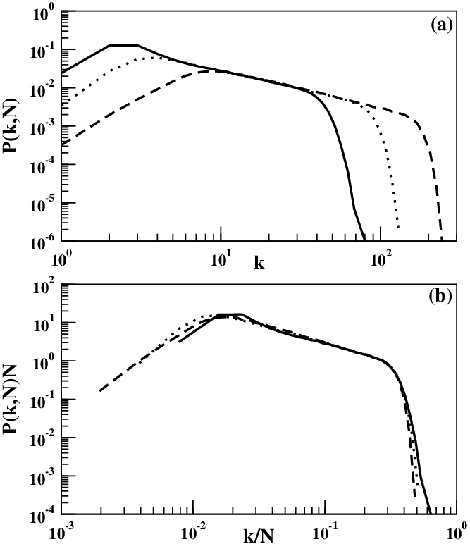
The nodal degree distribution has been calculated on the optimized network at the link density . From Fig. 1(c) we see that as . Consequently the degree distribution at is nearly the same as the Poisson distribution, the degree distribution of the MST. However, for finite link density the network becomes even more heterogeneous. This is manifested by the appearance of many small degree nodes and few large degree hubs. In Fig. 2(a) we have plotted the degree distribution for three different network sizes but at the same link density. The finite size scaling has been shown in Fig. 2(b) as
| (3) |
where and are used to obtain the best data collapse giving the degree distribution exponent . This clearly shows that at finite link density the resulting network is a scale-free network. At a different link density the exponent value is the same and the scaling range increases with the density. It is also observed that the model network is a small-world network from the density and beyond. It has already been reported that the air-route network of India has a scale-free structure [19].
We apply our model to the air-traffic network in India. There are =80 civilian airports in India for passenger transport. Considering all 12 airline companies [20] that are active in the air-space of India there are = 265 links connecting different pairs of airports [21]. Every airport is associated with a nearby city or town. We have collected the 2001 census (in India a general census is done every ten years) data for the populations of these cities from the website [22]. We have checked that indeed the available data for the top 185 populated Indian cities do follow Zipf’s law quite closely. The mutual distances of separation among these cities are calculated by the arc lengths of the great circles on the surface of the Earth joining pairs of cities. The latitudes and longitudes of these cities are available at the website [23]. Knowing these angles, the inter-city distances are obtained from
where miles is the Earth’s radius and the angles are measured in radians. As per our scheme we start by constructing an MST using as the weights. The total of 265 links are then dropped one by one using the optimized procedure described above until the link density in the real network is reached. Once the fully connected network has been formed we draw the airline networks for both the real as well as model data in Fig. 3(a) and 3(b), respectively. The visual similarity of these two figures is quite striking. However, on a closer look it seems that the links are more dense for the real network, though this is not true. Though the model network has exactly the same number of links as the real network, the longer links are more in the real network. This is because we started from an MST, and shorter links are selected in the very starting configuration.
For both networks we measure the nodal degree and the rank of every node. The degree vs. rank plot of the 80 node networks of India are compared between the real and model networks in Fig. 4(a). The comparison is good, and both seem to obey a power law of with and 0.75 for the real and model networks. Secondly, we study a one-to-one comparison of the real and model networks. For this purpose we calculate the factor and plot it with the rank in Fig. 4(b). We observe that remains limited within for 80 of the nodes. We conclude that the correspondence between the real and the model networks is quite good. To explore the dependence of our results on the parameter values we looked at the variation of the quantity within the range of and , and observed around 10-15 variation.
Finally, we would like to make three comments. (i) There could be a number of ways in which our study can be improved. The population in every city is distributed within a wide range of economic strengths. Only a fraction of population at the top edge of the distribution generally has access to air travel. Therefore perhaps it is better to replace the city population in our study by the number of people who are richer than a certain cut-off mark. We thought that an approximate estimate of this number would be the number of Income Tax payers. Using these numbers may make the analysis better provided they are not proportional to the city populations. Unfortunately we could not get city-wise statistics of Income Tax payers. Also, a city airport serves the neighboring towns and suburbs as well. Therefore an effective population of the city including its surroundings may be considered. (ii) This point, which is very interesting, was raised by a referee. In Fig. 4(b) there is a point whose is 9. Such a high value implies that the model degree is 10 times that of the real degree. We identified the city as Kanpur, which has a population of 2.7 million and occupies the 10-th position in the rank distribution. In spite of such a high population, Kanpur airport is connected only to Delhi and no other airport in the country, leading to its real degree being unity, but our model predicts it to be 10. A search on the Internet [24] reveals that indeed the traffic in Kanpur has increased to a high extent in recent years; there are modernization plans from the government and many other airlines are also planning to operate there. Therefore it is expected that the degree of Kanpur airport will eventually increase in the near future. This tendency has been correctly predicted in our model. (iii) The third point has also been raised by another referee. It may be interesting to explore if our method can be applied to the Indian Railway network as well. Recently it has been observed that such a network has the small-world property [25]. The main difference is that a large number of stations in a railway network are intermediate stations having two stations on the opposite sides. Therefore in the framework of our study two cities should be linked only if there is at least one train that starts at one city and finishes its journey on the other. Perhaps we will take up this study in a future project.
To summarize, we present evidence that a precise one-to-one reproduction of a network is possible once the key ingredients controlling the structure of the network are identified. We justify this claim by constructing an optimized transport network of inter-city traffic in which traffic is controlled by both the city populations (Zipf’s law) and by the rule of traffic distribution (Gravity law). The total cost function is determined by two competing factors, i.e., the cost of maintaining the traffic and the establishment cost of the network. This procedure has been applied to the airport network of India having 80 civilian airports, and a node-to-node comparison of the nodal degree values between the real network and the model network is made. The correspondence is found to be very good.
E-mail: manna@bose.res.in
References
- [1] R. Albert and A.-L. Barabási, Rev. Mod. Phys. 74, 47 (2002).
- [2] S. N. Dorogovtsev and J. F. F. Mendes, Evolution of Networks, Oxford University Press, 2003.
- [3] M. E. J. Newman, SIAM Review 45, 167 (2003).
- [4] G. Mukherjee and S. S. Manna, Phys. Rev. E 74, 036111 (2006).
- [5] M. Faloutsos, P. Faloutsos and C. Faloutsos, Proc. ACM SIGCOMM, Comput. Commun. Rev., 29, 251 (1999).
- [6] R. Albert, H. Jeong, and A.-L. Barabási, Nature 401, 130 (1999).
- [7] A. Barrat, M. Barthélemy, R. Pastor-Satorras, A. Vespignani, Proc. Natl. Acad. Sci. (USA), 101, 3747 (2004).
- [8] R. Albert, H. Jeong and A-L. Barabási, Nature, 406, 378 (2000).
- [9] M. T. Gastner and M. E. J. Newman, Phys. Rev. E., 74, 016117 (2006).
- [10] M. T. Gastner and M. E. J. Newman, Eur. Phys. J. B 49, 247 (2006).
- [11] M. Barthélemy and A. Vespignani, J. Stat. Mech. L07002 (2006).
- [12] G. K. Zipf, Human Behavior and the Principle of Least Effort (Addison-Wesley, 1949).
- [13]
Details in
en.wikipedia.org/wiki/Zipf's_lawandmathworld.wolfram.com/ZipfsLaw.html. - [14] J. Tinbergen, 1962, in Shaping the World Economy, Tinbergen, ed. New York: Twentieth Century Fund.
- [15]
K. Head, Gravity for Beginners, 2003,
economics.ca/keith/gravity.pdf. - [16] D. Jungnickel, Graphs, Networks and Algorithms in the series Algorithm and Computation in Mathematics; vol. 5. Springer, 1999.
- [17] J. B. Kruskal, Proceedings of the American Mathematical Society, 7, 48 (1956).
- [18] J. Hoshen and R. Kopelman, Phys. Rev. B., 1, 3438 (1976).
- [19] G. Bagler, Physica A 387, 2972 (2008).
- [20]
mapsofindia.com/india-domestic-flights.html. - [21]
mapsofindia.com/flight-schedule/index.html. - [22]
citypopulation.de/India-Agglo.html. - [23]
mapsofworld.com/lat_long/india-lat-long.html. - [24]
en.wikipedia.org/wiki/Kanpur_Airport,indianetzone.com/20/kanpur_airport.htm,siliconindia.com. - [25] P. Sen, S. Dasgupta, A. Chatterjee, P. A. Sreeram, G. Mukherjee and S. S. Manna, Phys. Rev. E., 67, 036106 (2003).