Still states of bistable lattices, compatibility, and phase transition
Abstract
A two-dimensional bistable lattice is a periodic triangular network of non-linear bi-stable rods. The energy of each rod is piecewise quadratic and has two minima. Consequently, a rod undergoes a reversible phase transition when its elongation reaches a critical value. We study an energy minimization problem for such lattices. The objective is to characterize the effective energy of the system when the number of nodes in the network approaches infinity. The most important feature of the effective energy is its ”flat bottom”. This means that the effective energy density is zero for all strains inside a certain three-dimensional set in the strain space. The flat bottom occurs because the microscopic discrete model has a large number of deformed states that carry no forces. We call such deformations still states. In the paper, we present a complete characterization of the ”flat bottom” set in terms of the parameters of the network. This is done by constructing a family of still states whose average strains densely fill the set in question.
The two-dimensional case is more difficult than the previously studied case of one-dimensional chains, because the elongations in two-dimensional networks must satisfy certain compatibility conditions that do not arise in the one-dimensional case. We derive these conditions for small and arbitrary deformations. For small deformations a complete analysis is provided.
keywords
Phase transformation in solids, Bi-stable lattice, Eigenstrain, Compatibility conditions.AMS
70C20, 74N15, 74Q05, 74Q15, 74A501 Introduction
This paper suggests a simple discrete model for phase transition theory. In two dimensions, we study deformation of bi-stable lattices (BL), which are periodic triangular networks of bistable elastic rods. A similar network with linearly elastic rods has been used by Cauchy, who formally averaged this assembly and obtained one of the first equations of continuum elasticity [8]. Here, we consider the same assembly, assuming, however, that the rods are bi-stable. The bi-stability models phase transitions: it is assumed that each rod has two equilibrium states that of length and , respectively. Here, can vary between and , so that a triangle of transformed rods still remains a triangle.
We believe that this bi-stable lattice model is the simplest and natural finite dimensional model for phase transitions in solids. Although it does not have all the features of continuum model, it appears to capture most of the expected features. At the same time this model allows for detailed description of inhomogeneous deformations and does not involve ad hoc assumptions of the continuum theory.
One dimensional chains of bi-stable rods are well investigated [1, 2, 10, 11, 15, 16]. Each bistable element can be in one of the two states (short and long mode) that differ by the equilibrium length. It is assumed for definiteness that initially all rods are in short mode and can transit to the long mode. The state of a chain with some transited elements is characterized by a scalar relative elongation, or one-dimensional strain, that is the normalized difference between the length in the deformed configuration and reference length.
Some results on the two-dimensional bi-stable lattices can be found in [12, 13] (explicit construction of certain special solutions, discrete Green functions), and [6, 7] (direct numerical simulations of time-dependent impact fracture problems). Other related problems are treated in the book [14] that also contains a wealth of additional references.
The present work differs from the above mentioned papers both in approach and in scope. It addresses the specific difficultly of the two-dimensional problem – compatibility conditions on the rods’ length. These conditions are automatically satisfied in one dimensional chains. In two-dimensional lattice, the transition of links to a new state generally leads to elastic deformation of all rods. For example, one transformed (elongated) rod does not fit into a triangular lattice of non-transformed (short) links without distorting the lattice. Each such distortion increases the energy of the assembly.
One of the objectives of the paper is to describe special lattice deformations that we call still states. These deformations carry zero forces in each rod, and thus the energy of each still state is zero. In any such state the length of each rod should be either or . Since the number of rods is larger than the number of nodes times the dimension, an arbitrary assignment of lengths may not correspond to an actual lattice deformation. Therefore compatibility conditions must be satisfied at a still state.
We describe the set of average strains of still states. First, we consider the network of rods undergoing arbitrary deformations. We assume that an effective strain tensor is represented by its eigenvalues. In the plane of eigenvalues, the set of all still states is a nonconvex curvilinear hexagon. We demonstrate structures that densely fill and derive nonlinear compatibility conditions.
Further, we consider the case of small deformation, linearize the compatibility conditions and develop the theory in more detail. We show that the linearized compatibility conditions are necessary and sufficient for existence of a lattice deformation with a given set of link elongations. In this sense, the conditions are analogous to the compatibility conditions in continuum elasticity. We also describe a sequence of still states whose average strains reach the average strain of any still state by incremental change of the structure starting from the reference configuration. This procedure can describe an evolutionary irreversible process of phase transition, such as the damage distribution. In this case, the initial state corresponds to ”undamaged” configuration and structural change – to irreversible damage propagation.
We also construct the set of all average strain tensors corresponding to still states and sets of deformed elements that densely fill that set. In the space of entries of the strain tensor, the set turns out to be a parallelepiped. We obtain explicit formulas that relate the side lengths and orientation of this parallelepiped to the non-dimensional critical elongation parameter , and three lattice direction vectors.
Finally, we suggest an equation for the effective energy density as a function of the total strain. It is as follows: if a strain is inside of the set , then the energy density is asymptotically close to zero as the number of the network nodes goes to infinity. If the strain is outside of this set, the energy density is proportional to the square of the distance between the strain tensor and .
The paper is organized as follows. Section 2 contains formulation of the problem and derivation of compatibility conditions for arbitrary deformations. Small deformation compatibility conditions are also obtained here. In Section 3 we describe several explicit constructions of still states for arbitrary deformations, as well as a set of eigenstrains of all still states. The remainder of the paper deals with the small deformation case. In Section 4.1 we formulate the problem. A new formula for average strain is obtained in Section 4.2. Unlike existing formulas that relate average strain to nodal displacements, our formula gives an expression in terms of rod elongations. This allows to relate components of strain to the average elongations along lattice directions. Such formulas seem to be of independent interest. In section 5 we provide a complete analysis of the compatibility conditions. In Section 6, we prove a characterization theorem for . This is done by constructing another family of still states called stripes. The eigenstrains of the stripes fill densely, in the sense that every strain within this set can be approximated by an average strain of some stripe, with an error of order where is the number of nodes. Section 7 contains a discussion of the effective energy density. Conclusions are provided in Section 8.
2 The problem
2.1 Energy of one bistable rod
Consider a bistable elastic rod with the energy that possesses two equal minima . Let us also assume that is convex outside of the interval , and its second derivative is positive in a proximity of each minima and . For definiteness, we may assume that the dependence of on the length is piece-wise quadratic or polynomial
| (2.1) |
where is the length of the rod in the reference configuration, is the length in the elongated mode, and .
The rods are elastic and locally stable in a proximity of the equilibria. The elastic force in the rod is
The rod has two equilibrium states and of equal energy
The magnitude of the force monotonically increases with the elongation in the proximity of equilibria.
There are several equilibrium lengths and for every in a proximity of zero. They are solutions of the equation

2.2 Triangular network
Consider a triangular periodic network made of the links defined above. For each node, there are six rods joining it with six neighbors. When the rods are of equal lengths, the network is elastically isotropic, its Poisson coefficient is equal to , [8]. The number of nodes in the period is three times less than the number of rods between them. There are three families of the parallel rods in the network
When the rods transit to a different state, the network becomes inhomogeneous (each rod can have a different length). We assume that the transition is periodic. Each period consists of nodes where can be arbitrary large. The network’s energy is the sum of energies stored in all links. The length of a link can be expressed through the position of its ends, that is the nodes. The nodes are determined by pairs of coordinates in a plane, or by parameters. Hence, the links’ lengths can not be arbitrary (for example, see Figure 2). We conclude that they are subject to compatibility conditions that we derive now.

2.3 Compatibility conditions
2.3.1 Necessary condition
There are conditions that constrain the lengths of the rods that can be joined in a hexagonal lattice. Consider an inner node in the lattice. There are six rods that link the node with the neighbors; let us denote the lengths of them as . Consider also six rods that surround the node forming a hexagon around it; let us denote the lengths of them as . These rods form six triangles joined at the node. The angles at the node will be denoted by .
The lengths of the listed twelve rods cannot be arbitrary. The sum of angles of the six triangles , .. is equal to ,
| (2.2) |
To express this condition in terms of the lengths, we use trigonometry. Cosine of each angle is expressed through the lengths of the links as
| (2.3) |
Here, . Therefore, the lengths of rods are constrained as follows
| (2.4) |
The number of these constraints is equal to the number of inner nodes in the structure.
2.3.2 Linearized compatibility conditions
In a linearized case when the lengths of the rods are close to , constraints (2.4) are simplified. Assuming that
| (2.5) |
we write as the function of , , :
Linearizing near
we find
Substituting this expression into (2.2), we obtain an elegant linearized compatibility condition for lattices
| (2.6) |
It states that the sum of the elongations of the spokes that come out of a node is equal to the elongation of the hexagonal rim around this node.
3 Eigenstrains and still states
3.1 Definitions
3.1.1 Still configurations
In this section we consider still configurations. These are deformed states with zero force in each rod. Because of the force-elongation dependence, this requires the length of each rod to be either or . To simplify presentation, in this section we scale and denote . Given a collection of such rod lengths, we call a configuration still if it is geometrically compatible, that is the ends of the link of the length one and can meet in the nodes. The examples of still configurations are given below in Figure 6. This section contains somewhat informal, but explicit description of the set of (average) eigenstrains of all still states corresponding to arbitrary (not necessarily small), deformations. We recall that eigenstrain is a generic name given to various non-elastic strains, such as strains due to thermal expansion, phase transformation, initial strains and so on.
Notice that the problem is reduced to a geometric problem of tiling of the plane with triangles of four types with the lengths of the sides being equal to , , . and , respectively.
Any still configuration can be split into parts that are also still configurations. Each configuration is characterized by a symmetric second-rank eigenstrain tensor which shows the change of the initial shape of a periodic cell. Assume that a unit square element of periodicity of an initial (non-transformed) network contains a very large number of triangles. After deformation, it changes its shape. Asymptotically, this element is close to a parallelogram. The eigenstrain tensor describes the shape of it: the lengths of its sides and the angle between them.
3.1.2 Eigenstrain of still states
Generally, a deformation due to transformation is followed by elastic deformation of all links due to compatibility conditions (2.4). Therefore, eigenstrain of the composite network is not a convex combination of eigenstrains of its components that are, in principle, incompatible and lead to additional distortions on the boundaries of components. The eigenstrain of a compatible configurations of still states is an affine function (the average) of the eigenstrains of the phases. It is independent of the structure of the mixture
| (3.1) |
where is the volume fraction of the phase with eigenstrain . The only role of the structure is the selection of compatible states.
Next, we describe the variety of still states.
3.2 The homogeneous still states
In the initial network, there are three families of codirected rods. The homogeneous still states are the states in which all the rods in one family are in either ”short” or ”long” mode.
3.2.1 Classification of homogeneous states
There are eight homogeneous states that consist of periodic arrays of equal triangles and their reverses.

- 1.
Initial state with the lengths of the links equal to . The elementary square of the state (the eigenstrain) is assumed to be an identity matrix,
(3.2) - 2.
The dual state with the lengths of the links equal to . The unit square element of the initial state is transformed to
(3.3) and it is still proportional to an identity matrix. We call the eigenstrain of the state .
- 3.
State with the lengths of the links equal to that consists of isosceles triangles. The square element of the initial state is transformed to
(3.4) Here, is the angle between the base of the isosceles triangle and its side, is expressed through as
is the eigenstrain of the state .
- 4.
Together with , there are two twin states, with the lengths of the links equal to and with the lengths of the links equal to . The eigenstrains of these states are obtained from by rotating it to the angle of , respectively.
(3.5) where is the rotation matrix.
- 5.
State with the lengths of the links equal to that consists of isosceles triangles. The square element of the initial state is transformed to
(3.6) Here, is the angle between the base of the isosceles triangle and its side, is expressed through as
The angles and are related as
- 6.
State is also accompanied by the two twin states, with the lengths of the links equal to and with the lengths of the links equal to . The eigenstrains of these states are obtained from by rotating it by the angle of , and , respectively.
(3.7)
Remark 1.
Pairs , and , are dual: each of them is transferred into another by mutually replacing rods of the length and .
3.2.2 Vertices of the eigenstrain states set
Consider a set of all possible eigenstrains. In a three-dimensional space where coordinates are entries of the eigenstrain tensor, this set is a bounded region. The eigenstrains of the homogeneous states correspond to the vertices of . Indeed, there the elongation of the each family of the rods is extreme, that is the deformation in the directions of the rods’ families is extreme. The rods cannot be elongated (contracted) in these directions without an elastic deformation. Therefore, there exist three trial matrices and of deformation that correspond to impossible change of eigenstrain in the sense that
does not correspond to any still state, for any .
Consider, for example, state . Set of impossible deformations contains a cone of matrices of the form
| (3.8) | |||
here is arbitrary. These deformations require contraction of one of the rods. In the state such contraction is impossible. The impossible deformations form a cone in the eigenstrain space. Similar cones can be established for all homogeneous states because the structure cannot be extended (compressed) in the direction of long (short) rods. Below we describe the two- and three-phase composites of still states. The eigenstrain of any still state composite is a convex combination of eigenstrains of its phases, therefore, the two-phase composites correspond to edges of and two-phase composites – to its phases. Set is a polyhedron.
We also describe a two-dimensional set of eigenvalues of eigenstrains. This set is also bounded and symmetric (includes pairs and ). The eigenstrains of the homogeneous states correspond to vertices of , and the differently oriented homogeneous still states , and (and , and ) correspond to the same pairs of eigenvalues – vertices of . However, the eigenvalues of a two-phase composite are convex combinations of eigenvalues of components only if their vertices are coaxial tensors (the eigen-axes are codirected). Otherwise, they are located along a curve that join the vertices. Therefore, is a symmetric curvilinear hexagon.
3.3 Laminate structures
There are still states composed from several basis homogeneous states. We call two still states and are called laminate compatible if lengths of their rods along the layers are the same. In terms of eigenstrains, the states are laminate compatible if a vector (the tangent) exists such that
| (3.9) |
that is, matrices and have the same tangent component. All pairs of homogeneous states except and can be laminated together, along the side of a common self-strain, if the states are allowed to rotate freely. We also remark that threads in laminate-compatible structures may possess kinks, as in Figure 4. The continuity of the angles is not required for compatibility of a lattice, in contrast with continuum mechanics.
3.3.1 Structures from an isotropic and anisotropic phases
States and are laminate compatible. The eigenstrains of mixture are
where is the volume fraction of phase , is the thickness of the layer, and is the thickness of the layer of phase . The laminate is shown in Figure 6.
In addition, the eigenstrains and are isotropic and therefore their eigenvectors are codirected with eigenvalues of any phase they are mixed with. A structure of one of them and another phase leads to average of eigenvalues of eigenstrain. The eigenvalues of are located at the straight line between eigenvalues of and .
Similar laminates can be built for , , , and . The eigenvalues of these structures span the intervals between the eigenvalues of the homogeneous states.


3.3.2 Laminates from two anisotropic phases and
Consider the compatibility of two anisotropic states . Each of them consists of ”long” and ”short” rods. Assume for definiteness, that tangent to laminates corresponds to the line of ”short” links. This line is an axis of symmetry for the state that consists of two families of long and one family of short rods. In orthogonal coordinates , the eigenstrain is diagonal, its eigenvectors are codirected with and .
The state (that consists of two families of short and one family of long rods) can be made compatible with if it is rotated so that its line consists of short rods. In other words, tensor of eigenstrain must be rotated to a proper angle so that its tangent entry becomes compatible with (3.4), , see compatibility conditions (3.9). The rotated matrix is computed from the additional conditions that trace and determinant are independent of rotation. The rotated eigenstrain becomes
where . Eigenstrain of the mixture is still an average of those in the phases according to (3.1).
| (3.10) |
where is the volume fraction, as before.
Eigenvalues of a composite are parametrized by . They depend on nonlinearly. In the eigenvalue plane, they are located at an arch that spans and , not at an interval between them.
3.3.3 Two-phase twins
Besides these structures, there are two-phase twins: the laminates of differently oriented phase or . These structures preserve the trace of and , respectively, and their eigenstrain is as follows
where , . One could check that the eigenvalues of these twins are never isotropic, Figure 4(b).
Together, all listed structures form a region in the plane of eigenvalues of . The boundary has three components corresponding to structures (an interval), (an arch), and (an interval) and four vertices, see Figure 5.

3.3.4 Three-phase laminates
There exist three-phase still structures with eigenstrains that densely cover the domain bounded by the eigenstrains of two-phase structures. Curvilinear triangular domain is covered with laminates from three phases, obtained by laminating the isotropic phase with the laminate . The tangents to laminates correspond to the sides of unit lengths in all three components. The eigenstrain is
where
The corresponding eigenvalue pairs cover the part of that lies outside the rectangle, three of whose vertices are in Figure 5.
3.4 Hexagon-triangles-strips
The central triangle can be covered by mosaic assembly from elements of , and differently oriented elements , shown in Figure 6. Notice that and are incompatible, and the assembly uses anisotropic elements between them. The assembly is as follows.
- 1.
First, three parallelograms from , and are formed of the sizes , , and , respectively. The links of the unit length form the base of each parallelogram and the links of the length form the sides (Figure 6, (a)).
- 2.
Second, these parallelograms are joined by the edges with the equilateral triangle with the side in between, forming the structure shaped as Y (Figure 6, (b)).
- 3.
Third, the obtained figure is copied and translated. The copies are joined by edges, leaving empty triangles and hexagons with the parallel sides of , and unit-length elements.
- 4.
Finally, the triangular parts are filled with and the hexagon parts with . The obtained periodic assembly covers the whole plane (Figure 6, (c)).
The obtained periodic assembly covers the whole plane.


The periodicity element consists of
– three parallelograms from , respectively, of , , and triangles each,
– two triangles composed of of triangles each.
– one hexagon containing of triangles.
Thus the element consists of
pairs of triangles.
The eigenstrain of the assembly is a sum of eigenstrains of its pieces,
| (3.11) |
where
| (3.12) |
3.4.1 Asymptotics
In particular, is isotropic if . Then
| (3.13) |
When and varies in , the isotropic deformation varies from one to .
The described structures degenerate into two-phase structures and . If , then
If and , we have
3.5 Covering of the whole domain
Together, the hexagonal and three-phase-laminate structures densely fill the whole curved hexagon of eigenvalues of still states. The two types of covers are met on the line when in hexagons and in three-phase laminates. . The covering is non-unique: For instance, one can replace with and with everywhere (complementary or dual replacement) and obtain another complete coverage. The density of the coverage is easy to estimate through the explicitly given parameters . The distance from an eigenstrain of a discrete periodic structure to the arbitrary point of the domain is of the order of , as follows from the above explicit formulas.
4 Small deformations
4.1 Linearized elongations
In the remainder of this paper we consider the case of small deformations which means that rod elongations are linearized near the reference configuration. The linearized relative elongation of the rod can be written as
| (4.1) |
where is the unit direction from node to node , and are the displacements of nodes and , respectively.
Consider a triangular periodic network of nodes, where is finite, even though it can be arbitrary large. We also suppose that the nodes are arranged into a hexagonal shape containing nodes along a side (see Figure 5.1 for an example).
Factoring out in (2.1) and using nodal displacements instead of the rod length, we write the energy of a rod as
| (4.2) |
where, is a dimensionless parameter characterizing the critical relative elongation. The graph of the dependence is shown on figure 7 (Compare with (2.1), where denotes the actual rod length).

The displacements in the equilibrium state are found by minimizing the total energy of the network:
4.2 Average strain
An effective homogeneous deformation state of the network is characterized by an average (linearized) strain tensor . In this section we obtain a formula for the average strain in terms of elongations .
Denote the number of nodes in the network by . Given a set of displacements of nodes we define a continuum deformation that coincides with at each . This can be done by interpolating. In the present case, the lattice forms a triangulation of the physical domain . Therefore it is easy to construct a piecewise linear interpolant, using finite elements. After this is done we obtain a continuous function such that
- •
for and being the position of node ;
- •
is linear on every elementary triangle of the lattice.
To we associate strain tensor :
Average strain is defined by the formula
| (4.3) |
where is the domain of and is
There exist formulas for in terms of displacements (see [4], [9]). However, for our purposes it is better to work with the relative elongations because we would often prescribe elongations, rather than displacements. To use standard formulas one would have to solve the system (5.1) (see the next section) that relates elongations and displacements. We choose a more direct route that involves relating three average elongations along the lattice directions with the three independent components of the average strain.
Rewrite (4.3) as
where is the set of elementary triangles of the network, is the number of elementary triangles in the network, and is the strain tensor on elementary triangle :
Since the average strain tensor is a symmetric matrix, it has three independent components:
Consider three lattice direction vectors , , and (see figure 8(a)):


We can find the components of using the values , . Hence, consider
| (4.4) |
Using linearity of on triangle for edge of the triangle we find
Given a triangle with vertices (see figure 8(b)) define vector as:
Using this notation we rewrite (4.4) as a linear system for finding the components of given elongations :
| (4.5) |
where the matrix is given by
| (4.6) |
and function by
Function is simply a linear 1-1 mapping from the space of three dimensional vectors to the space of symmetric matrices.
Further, we will rewrite the sum over triangles in (4.7) as the sum over edges (this is just the change in indexing). Denote all edges of the array by , all boundary edges of the array by and all non-boundary edges of the array by (). Then
where vector has the components defined by
Next, equation (4.7) can be rewritten as
Denote the average elongation by :
| (4.8) |
Then we rewrite (4.7) and obtain the desired formula for the average strain in terms of average elongations:
| (4.9) |
This formula is used extensively in the remainder of the paper. The first term in the right hand side contains contributions from all interior edges of the lattice, while the second term contains the contributions from the boundary edges only. As the number of nodes increases, the second term becomes a small perturbation of the first. This becomes clear from the following estimate
| (4.10) |
Here denotes the Frobenius norm of a matrix, and is the Euclidean norm. Note that the ratio
of the number of the boundary edges to the number of all elementary triangles goes to zero as the number of nodes approaches infinity.
5 Compatibility conditions
In the next two sections, we study the linearized version of the problem of finding still states. The linearized formulation is as follows. Equations (4.1) relating node displacements with link elongations can be concisely written as
| (5.1) |
where is a tuple of displacements , say , and is a tuple of . The number of unknowns in (5.1) is (since each has two independent components). The number of equations is larger, approximately (see Lemma 5.1 below for the exact count). Therefore, we have an overdetermined system (the number of unknowns is less than the number of equations). As a consequence, (5.1) may be unsolvable for some . The values of for which (5.1) is solvable are called admissible.
5.1 Compatibility conditions characterize range of
In this section we show that compatibility conditions (2.6) ar necessary and sufficient for solvability of (5.1). Necessity is clear from the derivation of (2.6), so we focus on sufficiency.
Suppose that we have the hexagonal array with a side of points (see figure 9).
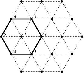
For every hexagon consisting of 6 vertices we formulate the condition (2.6): the sum of elongations of the outer edges equals to the sum of elongations of the inner edges. For example, for figure 9 the equation will be
The collection of all such equations will be called hexagonal equations.
Next, we need a preliminary result giving the exact count of the number of nodes, edges and hexagonal equations. The following lemma is used later to carry out proofs by induction.
Lemma 2.
The total number of nodes , the number of edges , and the number of hexagonal equations depend on as follows.
Proof.
We will prove the lemma using mathematical induction.
For we have a hexagon that has 7 vertices, 12 edges, and 1 hexagonal equation. Indeed,
Thus, the formulas are true for .
Suppose that given formulas are true for . Let’s prove that they are true for .
When we increase by 1 we “wrap” the array by a layer of points. Therefore, we add vertices, we allow new hexagonal equations, and add edges. Thus, the number of vertices for the size is:
the number of equations is
and the number of edges is
Since , , and , the formulas are true. ∎
Observe that
We know that for the mapping we have . This follows from the well known results on graph rigidity, in particular theorems on the first-order rigidity of triangulations (see e.g. [3] and references therein). Thus,
The hexagonal equations can be concisely written in the form
| (5.2) |
where is a matrix, ; -th row of this matrix corresponds to -th equation.
Lemma 3.
Matrix has full rank .
Proof.
We will restate the lemma in the form: all hexagonal equations are linearly independent.
We will prove the lemma in its new form using mathematical induction on . For we have . One equation is linearly independent.
Suppose, the lemma is true for . Let’s prove it for .
Increasing by 1 we wrap a hexagon of side size with a layer of points. Doing so we add some number of hexagonal equations to those that we had in the original hexagon. The hexagonal equations of the original hexagon are linearly independent. Each new hexagonal equation contains an edge that is present in no other equation. Thus, all equations are linearly independent. ∎
Since matrix has rank , we find . Thus,
| (5.3) |
Necessity of hexagonal equations implies that each admissible satisfies them. This fact can be stated as follows: for any we have . This in turn implies
| (5.4) |
Theorem 4.
For any vector satisfying there is a unique (up to translation and rotation) vector satisfying .
6 Still states and small deformation eigenstrains
In the small deformation case, a still state is a collection of nodal displacements ) satisfying equations (5.1) with the right hand side of special form. The components can take only two values: and , where is the critical elongation from (4.2). If we call the corresponding edge short, otherwise the edge is called long. To construct a still state, one could choose a length for each edge (long or short). The resulting configuration is accepted if the resulting triangles form a tessellation. Otherwise the configuration is rejected. In the case of small deformations, an admissible elongation vector should lie in the range of the matrix from (5.1). Equivalently, such must be a solution of the hexagonal equations (5.2).
Denote the set of all still states by . To characterize , one needs to solve the following problem.
Given with , find realizing that , that is, find such that .
This is possible only if satisfies hexagonal equations from Section 5. Complete characterization of seems very difficult, and is not addressed in this paper. The reason for the difficulty is the lack of a convenient structure. It is easily checked that is not a linear space, or even a convex set. Therefore, a description of this set cannot be obtained by linear algebra methods.
6.1 An algorithm of adding still states
In this section we characterize the set of strains that can be well approximated by the average strains of still states. An average strain of a still state can be conveniently described by a triple of concentrations of long edges parallel to the lattice directions. In this section we propose an explicit construction that furnishes a large number of still states. Concentrations of these states densely fill a certain unit cube in the concentration space. Our construction is based on two observations. First, one needs a binary operation that produces new still states by combining two already known still states. Second, one needs a simple ”building block”, that is, a still state that could be easily combined with its slightly modified (e.g. translated and rotated) replicas. In view of the linear structure of , the convenient operation is summation. However, summation of two still states does not always produce a still state. An additional condition that ensures that the sum of still states remains a still state is non-overlapping of the long edges (see Lemma 5 below): if a particular edge is long in the first state, then it should be short in the second state, and visa versa.
From this we deduce that the building block should have low concentrations of long edges, and the placement of these edges should be localized as highly as possible. If both of these requirements are satisfied, one can add together shifted copies of the building block to generate new still states with higher concentrations.
Lemma 5.
The sum of two still states and is a still state provided .
Proof.
Since and are still states, their components satisfy
for all connected nodes and . Moreover, the condition of orthogonality says that for each certain pair the values and cannot equal simultaneously. Thus,
Also, since and are still states, we have
where is the matrix of the hexagonal system (5.2). By linearity ,
Since the necessary conditions hold, the sum is a still state.
∎
For a still state in (4.10) we have . Thus
| (6.1) |
Theorem 6.
For any , , and any there exists a still state such that its concentrations , , satisfy
Proof.
To prove the theorem we will use special still states called stripes. These states have everywhere except for one stripe that has non-zero elements in one direction (figure 10). We can see that these stripes are still states because their components are either 0 or and they satisfy the hexagonal equations: each hexagon has either all zero elongations or one non-zero inner elongation and one non-zero outer elongation.


Observe, that for two different stripes and we have . In other words, the long edges of do not overlap the long edges of , and thus is a still state (figure 10(d)).
We have 3 different groups of stripes, , , and , one for each direction: one group of horizontal stripes and two groups of rotated stripes. The number of stripes in each group is .
Next, define the vectors , as follows. The dimension of is (the number of edges), and the components are equal to one if the corresponding edge is parallel to (a lattice direction vector), and equal to zero otherwise. It is easy to see that if for some then , , since each “stripe” has no more than long edges. Also, since each stripe has long edges only in -th direction, we get
This implies
First, we explain the main idea of the proof. Consider -th group (stripes of one certain direction). If we add all stripes of this group then we’ll get . For the still state we have . Therefore, adding stripes one by one we increase from 0 to 1 with steps less than . Hence, for any there exists a step when . Finally, since different directions are independent from each other, we can run this algorithm for and at the end add all still states together to get what we need. Next, we present the technical details.
For any subset of set we will define functions and by
Since , we have and for . Also, we define and , .
From the corollary of lemma 5 it follows that for any the value of function is a still state with concentrations .
Suppose we are given values , . Let’s define sets , , as
Having defined we define values , , by
Since the sets are finite, the sets are finite and the maximum exists. Therefore, the definition of is consistent.
Now if for some we have then and . From the definition of we have
Since , we get .
If for some we have then there exists .
From the definition of function we get
And, since has maximal value in , we have . Hence,
Now using
and
we get
Finally, for the still state defined by
we have
∎
Let us define a set :
| (6.2) |
where is the inverse of the matrix given by Eq. (4.6). Set is a convex polygon in the space of symmetric matrices, since it is an image of a cube under a non-singular linear transformation. The components of the elements of form a set shown on figure 11.


Theorem 7.
For any there exists a still state of the hexagonal array with a side of points such that average strain of this still state satisfies
Proof.
Let us now discuss the significance of the Theorem 6.3 for linking the microscopic (lattice-level) and macroscopic (continuum) models. First, it is of interest to understand how geometry of depends on the microstructure. We observe that is the image of a unit cube under a linear mapping defined in (6.2). The unit cube and the mapping are both independent of the lattice geometry and particulars of the microscopic force definition. The two microstructure-dependent quantities in (6.2) are the relative (non-dimensional) critical elongation and the matrix . The actual critical elongation is , where is the equilibrium edge length. Passing to the -limit requires proper scaling of with , a typical scaling being . In the most natural setting, should scale as . If that is the case, then as . The set in that case is independent of , and is a non-dimensional constant of the problem that determines susceptibility of the material to phase transition. The diameter of increases linearly with . The matrix determines orientation of in the strain space and provides the explicit dependence of on the lattice geometry. Indeed, by definition (4.6), depends only on the products of components of the lattice direction vectors .
If , then is the ”flat bottom” of the macroscopic energy density because, by Theorem 6.3, any strain in this set can be approximated by a still state eigenstrain and the error of this approximation vanishes in the limit . Since the energy of every still state is zero, and is fixed as , the conclusion follows.
7 Effective energy of the network
In the previous section, we described the set of all strains that corresponds to zero effective energy. Here, we suggest the effective energy equation that corresponds to strains outside this set.
The average elastic energy of the network without the transition is described by Cauchy formula [8]
where is the average strain of the network. Assume first that the transition state is fixed in one of the still states . In other words, assume that no Long-to-Short and Short-to-Long transition are allowed. Let us denote the total average strain as . This strain consists of an eigenstrain and elastic strain :
The network is elastically inhomogeneous. However, we will assume for simplicity that the elastic properties stay constant. We neglect the effect of density variation in the transition which is reasonable for small elongations . Under this assumption, the average elastic energy of the network is
Minimizing the energy over all still state strains , we conclude that, for each fixed , the energy density can be written as follows
| (7.1) |
Assume now that . The density becomes
| (7.2) |
Notice that is a convex linear combination of the energies of homogeneous states that correspond to the vertices of . This follows from convexity of and . Motivated by this, we suggest a representation for the effective energy density in the limit (-limit). By the well known argument [5], using density of piecewise linear deformations, it is enough to consider only linear deformations (equivalently, constant effective strains). For these strains,
| (7.3) |
Here are the eigenstrains corresponding to the corners of .
8 Conclusions
We studied the discrete model of solid-solid phase transitions. The model consists of a two-dimensional triangular periodic lattice of nonlinear bi-stable rods. In order to characterize the effective energy of the lattice, we obtained the description of the set of the average eigenstrain tensors corresponding to so called still states, e.g. microstructure deformations that carry no forces. We also proposed several explicit constructions of such states for small and large deformations.
The compatibility conditions for rod elongations were derived. In the small deformation case, these conditions are necessary and sufficient for the existence of a deformation realizing a given set of elongations. To characterize the states with zero effective energy, we proposed a construction of a special class of still states. The eigenstrains of these special patterns densely cover the set of all eigenstrains corresponding to still states. We showed that the set for our network is a parallelepiped in 3D space of independent components of the strain tensor. The orientation and side lengths of were explicitly described in terms of the parameters of the underlying microscopic discrete model: the side lengths are proportional to and orientation is determined by the components of the lattice direction vectors via the matrix . Components of the inverse matrix are defined via components of the direction vectors according to (4.6).
The above results suggest the following properties of the energy density:
- •
if a strain is inside of , then the energy density is asymptotically close to zero as the number of the lattice nodes approaches infinity;
- •
If the strain is outside of this set, the energy density is proportional to the square of the distance between the strain and .
References
- [1] N. Ansini, A. Braides, and V. C. Piat, Interactions between homogenization and phase-transition processes, Tr. Mat. Inst. Steklova, 236 (2002), pp. 373–385.
- [2] N. Ansini, A. Braides, and V. C. Piat, Gradient theory of phase transitions in inhomogeneous media., Proc. Roy. Soc. Edin. A, 133 (2003), pp. 265–296.
- [3] K. A. Ariyawansa, L. Berlyand, and A. Panchenko, A network model of geometrically constrained deformations of granular materials, Networks and Heterogeneous Media, 3 (1) (2008), pp. 125–148.
- [4] K. Bagi, Stress and strain in granular asseblies, Mechanics of Materials, 22 (1996), pp. 165–177.
- [5] A. Braides, Gamma-convergence for Beginners, Oxford University Press, 2002.
- [6] A. Cherkaev, V. Vinogradov, and S. Leealavanichkul, The waves of damage in elastic lattices with waiting links, Design andf Simulation Mechanics of Materials, 38 (2006), pp. 748–756.
- [7] A. Cherkaev and L. Zhornitskaya, Protective structures with waiting links and their damage elovulion, Multibody System Dynamics, 13 (2005), pp. 53–67.
- [8] A. E. H. Love, A treatise on the mathematical theory of elasticity, New York Dover Publications, 1977.
- [9] M. Sataki, Tensorial form definitions of discrete-mechanical quantities for granular assemblies, International Journal of Solids and Structures, 41 (2004), pp. 5775–5791.
- [10] L. Slepyan, A. Cherkaev, and E. Cherkaev, Transition waves in bistable structures. i. delocalization of damage, Journal of the Mechanics and Physics of Solids, 53 (2005), pp. 383–405.
- [11] , Transition waves in bistable structures. ii. analytical solution: wave speed and energy dissipation, Journal of the Mechanics and Physics of Solids, 53 (2005), pp. 407–436.
- [12] L. I. Slepyan and M. V. Ayzenberg-Stepanenko, Some surprising phenomena in weak-bond fracture of a triangular lattice, J. Mech. Phys. Solids, 50(8) (2002), pp. 1591–1625.
- [13] , Localized transition waves in bistable-bond lattices, J. Mech. Phys. Solids, 52 (2004), pp. 1447–1479.
- [14] L. Splepyan, Models and Phenomena in Fracture Mechanics, Sprnger-Verlag, 2002.
- [15] L. Truskinovsky and A. Vainchtein, Kinetics of martensitic phase trasformations: lattice model, SIAM Journ. Appl. Math., 66(2) (2005), pp. 533–553.
- [16] , Quasicontinuum models of dynamic phase transitions, Continuum Mechanics and Thermodynamics, 18 (2006), pp. 1–21.