I am very grateful to the following people for their support, influence and for sharing with me many ideas about Physics during my Ph.D.: Jaume Garriga, Enrique Álvarez, Cedric Deffayet, Gia Dvali, Enric Verdaguer, Roberto Emparan, Jorge Russo, José Ignacio Latorre, Joan Soto, Joaquim Gomis, Guillem Pérez-Nadal, Daniel Arteaga, Tasos Avgoustidis, Manuel Asorey, Oriol Pujolàs, Michele Redi, Javier Redondo, Carla Biggio, Eduard Massó, Antón Faedo, Albert Roura, Andi Ross, Gregory Gabadadze Alberto Iglesias, Gastón Giribet, Zurab Berezhiani, Denis Comelli, Luigi Pilo and Frabizio Nesti.

Chapter 1 Conventions

Throughout the dissertation we will follow the Landau-Lifshitz time-like conventions; the $n$ -dimensional flat metric in particular, reads $\eta_{\mu\nu}=\mathrm{diag}\,(1,-1,\ldots,-1)$ . $n$ is the space-time dimension that will be taken to be 4 in some parts of the Thesis. We will also use $N=n-1$ as the space dimension. Lagrangians are written in momentum space as well as in configuration space, depending on the context. It is usually trivial to shift from one language to the other. For the totally antisymmetric tensor we choose $\epsilon^{0123}=1.$

We will define the Laplacian operator as $\Delta=\sum_{i}\partial_{i}\partial_{i}=-\partial^{i}\partial_{i}$ and $\Box=\eta^{\mu\nu}\partial_{\mu}\partial_{\nu}$ .

Given a connection, the Riemann tensor will be defined as

R^{\alpha}_{\phantom{\alpha}\mu\beta\nu}\equiv\Gamma^{\alpha}_{\phantom{\alpha}\mu\nu,\beta}-...,\quad R_{\mu\nu}\equiv R^{\alpha}_{\phantom{\alpha}\mu\alpha\nu}.

(1)

Similarly, given a spin-connection $\omega_{\mu ab}$ ,

R_{\mu\nu ab}(\omega)=\partial_{\mu}\omega_{\nu ab}-\partial\omega_{\nu ab}+\omega_{\mu a}^{\phantom{\mu a}c}\omega_{\nu cb}-\omega_{\nu a}^{\phantom{\mu a}c}\omega_{\mu cb}.

(2)

The (anti)symmetrization is performed with a weight factor,

\phi_{(ab)}=\frac{1}{2}\left(\phi_{ab}+\phi_{ba}\right),\quad\phi_{[ab]}=\frac{1}{2}\left(\phi_{ab}-\phi_{ba}\right).

(3)

The gamma matrices in 4-dimensions will be (see also [dWF84])

\displaystyle\gamma^{0}=\left(\begin{array}[]{cc}1&\ 0\\ 0&-1\end{array}\right),\quad\gamma^{i}=\left(\begin{array}[]{cc}0&\sigma^{i}\\ -\sigma^{i}&0\end{array}\right),\quad\gamma_{5}=\mathrm{i}\gamma^{0}\gamma^{1}\gamma^{2}\gamma^{3},\quad\quad C=\mathrm{i}\gamma^{2}\gamma^{0},

satisfying

\{\gamma^{\mu},\gamma^{\nu}\}=2\eta^{\mu\nu}.

(9)

We would also like to write a list of some abbreviations that appear throughout this Thesis:

•

Eq.: equation,
•

KK: Kaluza-Klein
•

PDoF: Propagating degree(s) of freedom,
•

EoM.: Equations of motion,
•

GR: General relativity,
•

CC: Cosmological constant,
•

RS: Rarita-Schwinger,
•

FP: Fierz-Pauli,
•

TDiff: Transverse diffeomorphisms,
•

Diff: Diffeomorphisms,
•

GCT: General coordinate transformations,
•

r.h.s.: Right hand side.

The references are sorted alphabetically.

\setchapterpreamble

[o]\dictum[Silvio Rodríguez]Lo más terrible se aprende en seguida y lo hermoso nos cuesta la vida.

Chapter 2 Introduction

In this Chapter, we will first review some of the proposals for modifying gravity at large distances, explaining the difficulties that appear in these models together with possible solutions. In the second part of the chapter, we present an outline of the rest of the Thesis.

1 Massive gravity and related models of modifications of gravity

The non-renormalizability of Einstein’s theory of general relativity (GR) suggests that GR will be superseded by a quantum theory of gravity at high enough energies with respect to a certain mass scale $M_{QG}$ . For dimensional reasons, it is customary to associate this scale with the Planck mass¹¹ 1 Source http://physics.nist.gov/.

M_{P}=\sqrt{\frac{\hbar c}{G}}=1.220892(61)\cdot 10^{19}\ \mathrm{GeV\cdot c^{-2}},

or the corresponding Planck length $l_{P}=GM_{P}c^{-2}=1.616252(81)\cdot 10^{-35}\ \mathrm{m}$ . The standard assumption is that GR is valid as an effective field theory (EFT²² 2 For reviews on EFT see e.g. [Bur04, Don95, Bur07, Gol07, Pol92] (see also [Fal07]). Henceforth, we will take units such that $\hbar=c=1$ .) for length scales much larger than $l_{P}$ . If this is true the expectation of learning something about the actual theory of quantum gravity from experiments to be performed within the near future is almost hopeless³³ 3 It is true that there are some astrophysical phenomena that involve very high energy events, and that may shed some light at energies beyond the possibilities of accelerators (see e.g. [A+07])..

Yet, when the cosmological observational data is analyzed within the framework of GR, the most successful models imply the existence of a vacuum energy $\Lambda$ whose magnitude is unnatural from the EFT point of view⁴⁴ 4 The value of a constant is technically unnatural if it is much smaller than the size of quantum corrections to it.. Hence, a very fine-tuned vacuum energy (or dark energy) is needed to reconcile GR with the observations [Wei00, Wei89] (see [Nob06] for a quite comprehensive review of the cosmological constant (CC) problem). This problem is rather pressing as it corresponds to the explanation of actual data [S+07, AM+08, A+06]. In fact, the problem can be divided into two: first why the vacuum energy is not as high as it should be (fine tuning problem) and second why is it so small that becomes dominant precisely at the present time (coincidence problem). For a modern review article see, e.g., [CST06].

To address the previous problems, GR can be modified at short (ultraviolet, UV) or long (infrared, IR) distances. This requires the introduction of new length scales $L$ in the theory which can be combined with $l_{P}$ to build new constants with dimensions of length

L_{q}=l_{P}\left(\frac{L}{l_{P}}\right)^{q}.

(1)

When $L$ and $l_{P}$ are very different, we find a hierarchy of length scales larger than the Planck length where GR may be modified. For instance, we may assume that the fundamental scale of quantum gravity is a certain $L_{q}$ in (1), and that $l_{P}$ is a derived quantity. The energy scale at which quantum gravity effects are important, $L_{q}^{-1}$ , may be as low as TeV in which case the phenomenology of LHC could probe the true quantum theory of gravity and shed some light in the existing hierarchy between the Planck energy and the electroweak energy [AHDD98, AHDD99, AAHDD98]. Later on, we will discuss some models where this possibility is realized.

A related possibility is that there exists a certain low energy scale $L_{ir}^{-1}$ below which GR may be modified. In particular, if this length scale $L_{ir}$ is of the order of the present cosmological horizon, $L_{ir}\sim 10\ \mathrm{Gpc}$ , we expect modifications of GR to be important at current cosmological scales. Thus, all the predictions of GR at these scales (including the existence and amount of dark energy) may be modified within this new framework of infrared modifications of gravity.

Linearized Massive Gravity

The appearance of the length scale $L$ can be motivated in several ways. One of the first possibilities dates back to the work of Fierz and Pauli [FP39] and consists of adding a mass to the graviton. More concretely, if one considers a small gravitational field propagating in Minkowski space-time,

g_{\mu\nu}=\eta_{\mu\nu}+h_{\mu\nu},

(2)

the Lagrangian for the perturbations $h_{\mu\nu}$ corresponds to that of a massless particle of spin-2 [Ein16, FP39, Wei72]. In the linear approximation, one can solve the field equations for $h_{\mu\nu}$ in the presence of a conserved energy-momentum tensor⁵⁵ 5 In the massless case the energy-momentum tensor must be conserved from consistency reasons. and Newton’s law and the deflection of light for weak gravitational fields are recovered [Wei72, Ort04]. The interaction between two sources can be understood as due to the exchange of a massless particle so that, ignoring the tensor structure, the corresponding potential between two test particles of mass $m_{1}$ , $m_{2}$ can be written as

V(r)\sim\frac{m_{1}m_{2}}{M^{2}_{P}}\frac{1}{r}.

(3)

After the addition of a mass term to the mediator of gravity we expect that the potential will acquire a Yukawa form for length scales larger that the inverse of the mass scale. Namely, we expect it to behave as

V(r)\sim\frac{m_{1}m_{2}}{M^{2}_{P}}\frac{e^{-mr}}{r}.

(4)

If the mass is as small as $m\sim(10\ \mathrm{Gpc})^{-1}\sim 10^{-33}\ \mathrm{eV}$ , we expect that gravity fades away at cosmological distances and that at smaller distances the usual predictions of GR are recovered. This would imply that sources of the scale of the Universe would gravitate less than those smaller than this scale, which could alleviate the CC problem.

There are some obstacles in the way of this naive expectation. Assuming the Diff invariant kinetic term, there is only a possible mass term at the linear level which respects Lorentz invariance and does not contain ghost degrees of freedom⁶⁶ 6 By a ghost we mean a field with negative kinetic energy in the Lagrangian. [FP39],

{\mathcal{L}}_{m}\sim h_{\mu\nu}h^{\mu\nu}-h^{2}.

(5)

The interaction between two conserved sources computed from this linearized Lagrangian suffers from a discontinuity with respect to its massless counterpart, coming from the different tensor structure of the propagator. As shown in [vV70, Zak70], when coupled to conserved sources, the propagator of the massive theory reduces to

P_{\mu\nu\rho\sigma}=\frac{1}{k^{2}-m^{2}+\mathrm{i}\epsilon}\left(\eta_{\mu(\rho}\eta_{\nu)\sigma}-\frac{1}{a}\eta_{\mu\nu}\eta_{\rho\sigma}\right),

(6)

with $a=(n-1)$ where $n$ is the dimension of the space-time. In the massless case, the propagator corresponds to the massless limit of (6), but with $a=(n-2)$ , which means that the propagator of the massless theory does not agree with the massless limit of the massive case. This fact, known as vDVZ discontinuity, has drastic consequences. From measurements of the deflection of light by the Sun, the linear massive case can be excluded completely for any value of $m$ [vV70, Zak70]. Notice that the difference between the massless and the massive case comes from the scalar part of the propagator. One may think that the massless case can be recovered by adding a scalar field coupled to the trace of the energy-momentum tensor. This is obviously true, but the fact that $a(m=0)>a(m\neq 0)$ implies that the new field will be a ghost⁷⁷ 7 If non-local couplings are considered, the previous argument can be circumvented by choosing a coupling of the scalar field to matter that vanishes in the UV. Recently, a local model with a running $a$ has been discovered in certain local brane models with two extra dimensions, but the vDVZ discontinuity is still present [dR+07]., i.e. its propagator will have a negative residue [Zak70]. The existence of these states with negative norm destroys unitarity, and it is usually understood that quantum theories with ghosts are ill-defined. One can modify the quantization procedure to get rid of the the negative norm states but in this case the vacuum is unstable. In Lorentz-invariant theories its decay rate is in fact infinite⁸⁸ 8 If a Lorentz breaking cut-off is introduced in the theory, the decay rate can be regularized to be consistent with the observations. Similarly, as the linearized theory is understood as an effective field theory valid to a certain scale, beyond this scale new degrees of freedom can make the theory well-behaved [CNPT05]. [CJM04].

As first noticed in [Vai72], another way in which the discontinuity may disappear is through the non-linear effects. The main idea is that there is a source dependent scale $r_{\star}$ below which the three graviton vertex (i.e. the operators involving three gravitons) becomes of the same order as the quadratic terms and the classical linearized approximation breaks down. In other words, in the presence of a source the theory is strongly coupled for distances smaller than $r_{\star}$ . If $r_{\star}$ is bigger than the length scales at which an experiment probing gravity is performed, one must solve the whole non-linear system to give reliable predictions and there is a chance that the nonlinear effects restore agreement with GR. For the massless case, given a source of mass $M$ , the non-linear effects of GR become important at a scale $r_{\star}\sim r_{s}\equiv MM_{P}^{-2}$ , which for the Sun is much smaller than the distance at which the light deflection is measured. Naively, we would think that for length scales smaller than $m^{-1}$ , the dynamics of the massive case would be similar to the massless one, and that non-linear effects will not show up for $r>r_{s}$ also for the massive case. However, as found in [Vai72], this naive expectation is incorrect. It was shown in [AHGS03] (see also [DDGV02, NR04]) that for the FP massive case the spin-0 polarization of the massive graviton interacts strongly (in the presence of a source of mass $M$ ) at a scale which can not be smaller than

r_{\star}\gtrsim(m^{-2}MM_{P}^{-2})^{1/3}.

(7)

This scale diverges for $m\rightarrow 0$ . For a source of Solar mass $M\sim M_{\odot}$ and $m$ of the order of the Hubble length, $r_{\star}$ is larger than the size of the Solar System ( $r_{\star}\sim 10\ \mathrm{pc}$ ). The tensor structure of the massive graviton at distances $r\ll r_{\star}$ where non-linear effects are important is still an open issue. For a related model that we will discuss later (DGP), it was argued that the correct tensor structure is recovered and the vDVZ discontinuity is not present [DDGV02, Dva06] (see also [DKP03]).

Even if this effect is welcome, it is intimately related to another potential disaster of the theories that modify GR in the infrared: strong coupling at the quantum level. This pathology shows up when one considers the scale at which sources of the scale of quantum gravity are strongly coupled [AHGS03] (see also [Aub04] for an explicit calculation). From (7) we see that this scale is $\Lambda\sim(m^{2}M_{P})^{1/3}$ which for $m$ of the order of the present Hubble parameter is of the order of $\Lambda\sim(1000\ \mathrm{km})^{-1}$ . This energy scale is much lower than the Planck mass and also than the naive scale that one would expect from the analogous calculation for spin-1, $\sqrt{mM_{P}}$ . The reason why this happens is that the strongly coupled polarization does not have a standard kinetic term, but gets it from its mixing with other polarizations [AHGS03].

In a non-renormalizable theory like the one at hand, quantum corrections imply the presence of an infinite tower of higher dimensional operators suppressed by inverse powers of the interaction scale $\Lambda$ and a theory of quantum gravity would be needed to deal with calculations at distances smaller than $\Lambda^{-1}\sim 1000\ \mathrm{km}$ . These conclusions depend on the UV completion of the theory and, as outlined in [NR04], there may exist a non-generic prescription to choose the counterterms in such a way that the quantum corrections are not important in all the astrophysical situations (see also [Dva04]). In other words, the loop expansion may admit a resummation such that the scale $\Lambda^{-1}$ is unphysical (indeed, this is what happens for the classical expansion [Dva04]).

To sum up, let us state again that whenever a Lorentz invariant theory has a massive graviton as the mediator of gravity, it requires the presence of strong coupling to be phenomenologically acceptable, which generically requires a UV completion at very low energy scales.

A related aspect of massive gravity is that when propagating on a curved background, it behaves differently than in flat space⁹⁹ 9 Writing the action for a spin-2 field in an arbitrary background is problematic as the structure of the constraints is modified and a ghost mode may appear or causal propagation can be lost (see, e.g. [AD80]). These problems have been recently reconsidered in [BGKP00] for the coupling of the spin-2 field to gravity (see also [PR08, DH07, AD71] where the coupling of spin-2 fields to electromagnetism is studied).. In particular, in anti-de Sitter (AdS) space there is no vDVZ discontinuity [KMP01a, Por01, KKR01] while in de Sitter (dS) a light massive graviton becomes a ghost [Hig87]. The reason why this happens is simply that the mode that becomes strongly coupled in the flat case acquires a kinetic term proportional to the curvature in the curved background case¹⁰¹⁰ 10 As shown in [DDLS01], the discontinuity reappears at the quantum level, but then its effects happen at very short distances. [AHGS03].

For the sake of completeness, we should mention that there are some theories with massive gravitons which only involve the four dimensional metric and are invariant under diffeomorphisms. An example of these theories is gravity with higher derivatives [Ste78, Ste77, Sta80, DFMW08, NO07]. One can show that the spectrum of this theory can be decomposed into a massless graviton and a massive graviton with a mass term different from (5) in general. In this sense, these models resemble bigravity theories (see below).

However, these models have a very serious drawback, namely the appearance of ghost states. Only in certain instances where the massive states disappear this pathology may be absent. In these cases, called Modified Gravity Models, the term in higher derivatives is simply $f(R)$ and the theory is equivalent to a scalar-tensor theory (cf. [Wan94, Ste78]). The gravitational interaction can be modified both at long and short distances¹¹¹¹ 11 The modification at large distances occurs, e.g., when one considers functions of the form $R^{a}$ , with $a<1$ [Woo07]. but a successful model is still absent [DFMW08]. Yet another possibility is provided by topological massive gravity in $2+1$ dimensions [DJT82b, DJT82a] or the possibility of mass generation through matter loops in AdS [Por02]. Besides, we could also consider non-local modifications of gravity [DHK07, AHDDG02, Dva06].

Non-linear Massive Gravity

From the discussion above, it seems clear that it is essential for any theory of massive gravity to have a formulation beyond the linear regime. In fact, this is also true for the massless case both from observational (perihelion of Mercury) and theoretical (the equivalence principle) considerations. In the massless case, the gauge invariance can be a guiding principle in this extension and it is usually stated that the only consistent final result is GR in the usual geometrical formulation (i.e. having the whole group of diffeomorphism as a gauge group) [Kra55, OP65, BDGH01, Wal86, Des70, Fey95, Gup57]. The presence of the mass term (5) breaks the gauge invariance of the linear theory and it is not clear how to build a non-linear theory consistently. One could consider adding a term to the full GR Einstein-Hilbert Lagrangian that in the weak field limit reduces to (5). Since no scalar can be built out of the metric alone without including derivatives, either one relaxes the invariance under diffeomorphisms, or other dynamical fields should be added to the theory (see below). A possibility in the first approach consist of adding a static background (e.g. Minkowski space-time) and defining $h_{\mu\nu}$ and the mass term as in (2) and (5). However, in this case, besides breaking of the background independence of the theory, the Hamiltonian is not bounded from below. This can also be understood through the appearance of a mode with a negative kinetic energy which propagates at the nonlinear level (Boulware and Deser mode) [BD72, CNPT05] (see also [GG05a]). A related problem of this proposal is that the spherically symmetric solution with flat boundary conditions¹²¹² 12 Remind that, in general, the Birkhoff theorem does not hold in modified theories of gravity [Ste78, DMS07]. presents a singularity at finite radius [DKP03] (see also [JK86]).

An approach more similar to the massless case can be followed, based on the Stückelberg formalism of compensators for massive gauge theories [Stü38] (see [RRA04] for a review). Currently, this approach has been developed until third order [Zin07]. Besides, a version of the Brout-Englert-Higgs mechanism to give mass to vector fields can be applied to spin-2 [tH07]. The idea in both cases is to add new degrees of freedom coupled to the massive graviton in a way that the theory has a gauge invariance which makes them spurious. The presence of a gauge invariance at linear order may then be used to guess the non-linear terms as the non-linear extensions of linear gauge invariance must satisfy certain consistency conditions, such as the closure of the associated algebra [Hen98]. Both approaches encounter problems with unitarity, which may be understood from the counting of the degrees of freedom. The number of new fields required for a diffeomorphism invariant formulation of massive gravity is 4, whereas the massive and the massless theories differ by just 3 degrees of freedom. This means that besides the spin-2 degrees of freedom, the gauge invariant formulations generically include a new scalar. This field must be a ghost in flat space since the only ghost-free possibility for Lorentz invariant massive gravity only has tensor degrees of freedom and this destroys the consistency of the theory (see, however, [Por02] for a successful model in AdS).

The Fierz-Pauli mass term is singled out from the rest of Lorentz preserving mass terms because at the linear level this new degree of freedom disappears in Minkowski space. This allows for a successful Stückelberg formulation of massive gravity at linear order [AHGS03]. However, the dangerous ghost mode reappears once the non-linear effects are taken into account [BD72]. Furthermore, around non-trivial sources the ghost is also present at the linear level [CNPT05]. In particular, this means that for the Fierz-Pauli mass term any non-linear extension breaks down at length scales beyond the radius where the non-linear effects can cure the vDVZ discontinuity.

The previous negative conclusions may change if Lorentz invariance is broken [GG05a] (see [RT08] for a review). In that case, there are more possibilities for mass terms which are unitary and are not affected by strong coupling [Rub04, Dub04] (see also [DPR07, BFK08, Jac07] for other aspects of Lorentz violation and gravity). As the mass term explicitly breaks Lorentz invariance, the massive polarizations do not necessarily correspond to spin states. This kind of models appears naturally when more fields are added to GR, and bigravity (to be discussed below) is perhaps the simplest possibility¹³¹³ 13 Another possible generalization is to consider non-local extensions [DGS03, Dva06]..

Large Extra Dimensions and Braneworlds

From the previous section, it seems clear that a covariant non-linear theory with massive gravitons requires the presence of new fields coupled to the graviton. The theories with extra spatial dimensions provide such fields as the pure massless graviton in higher dimensions can be understood as a four dimensional field theory with an infinite tower of modes interacting with each other¹⁴¹⁴ 14 Besides, the presence of extra-dimensions is necessary for consistent string theory [Pol98]. [ACF87]. This provides a method to find consistent coupling of massive gravitons in fixed backgrounds [AN89, NW89]. Nevertheless, it should be noted that those completions are not consistent in general unless the infinite tower of modes is considered [DPS89].

The simplest possibility is that the extra dimensions are compact with a typical size $L$ . In this case, the extra dimensions can be understood as a massless graviton coupled to a discrete tower of massive fields with masses depending on the size and topology of the compact manifold [AHCG01, ACF87]. If two test masses $m_{1}$ , $m_{2}$ are placed within a distance $r\gg L$ the gravitational flux lines can not spread in the extra compact dimensions. Only the massless mode is excited at this energy scale and the usual four dimensional potential potential (3) is obtained,

V(r)\sim\frac{m_{1}m_{2}}{M^{2+d}_{Pd}L^{d}}\frac{1}{r},

(8)

where $d$ is the number of extra dimensions and $M_{Pd}$ is the gravitational scale of the theory. The effective four dimensional Plank mass in this set-up is easily read comparing the previous expression with (3),

M^{2}_{P}=M^{2+d}_{Pd}L^{d}.

For distances of the order $L$ and below, the gravitational interaction is modified by the tower of massive modes. The fact that Newton’s law has not been probed at distances smaller than than $10^{-2}$ millimeters [D+07, GSW+08, K+07] allows for a $L\sim 10\ \mu\mathrm{m}$ and a fundamental Planck mass $M_{Pd}\gtrsim 1\ \mathrm{TeV}$ for $d\geq 2$ [K+07, AHDD98].

If the Standard Model fields live in the bulk, the Kaluza-Klein (KK) reduction affects all the interactions. However, the Standard Model interactions have been accurately measured at the weak scale $m_{EW}\sim 1\ \mathrm{TeV}$ and this gives the constraint $L<m^{-1}_{EW}\sim\ 10^{-17}\ \mathrm{mm}$ .

A way to circumvent the previous arguments is by localizing the Standard Model fields in a four dimensional submanifold of a certain width $L_{D}$ (domain wall or brane) [RS83, AHDD98, DS97]. This idea introduces two length parameters apart from the Planck length: the size of the extra dimensions $L$ and the width¹⁵¹⁵ 15 This length scale can be arbitrarily small. of the defect $L_{D}$ . If gravity is not localized, these parameters can be chosen so that gravity is modified at the submillimeter scale and the compact extra dimensions are large in comparison with the electroweak scale. In this scenario, gravity is modified at high energies and remains massless and four dimensional at large distances¹⁶¹⁶ 16 Another way of localizing fields in submanifolds is provided by string theory and $D$ -branes [Pol98]..

An alternative to the existence of compact dimensions is provided by warped extra dimensions (not necessarily compact but of finite volume and with the Standard Model fields localized in a brane) [RS99a, RS99b] (see [Maa04] for a review). In this scenario, known as Randall-Sundrum scenario, the extra dimensions are not factorized and solutions with nontrivial warped factors of typical curvature $L_{W}^{-1}$ exist and give rise to massless zero modes and a continuous tower of massive states without a mass gap. Nonetheless, the gravitational interaction is again four dimensional for length scales larger than $L_{W}$ . The effect of the warped factor can be understood as a potential that makes the wave functions of massive states to be suppressed in the brane, and the final effective non-relativistic potential for two sources in the brane can be written as

V(r)\sim\frac{m_{1}m_{2}}{M_{P}^{2}}\frac{1}{r}+\frac{m_{1}m_{2}}{M_{P}^{2}}L_{W}^{2}\int_{0}^{\infty}\mathrm{d}m\ m\frac{e^{-mr}}{r}=\frac{m_{1}m_{2}}{M_{P}^{2}}\frac{1}{r}\left(1+\frac{L_{W}^{2}}{r^{2}}\right).

(9)

From the previous expression we see that a mass gap in the spectrum in not required to obtain a correct Newtonian limit because the coupling of massive modes to matter is suppressed by a factor $mL_{W}^{2}$ . Again, this model proposes modifications to the gravitational interaction only at high energies.

There are many generalizations of the previous model, and we would like to focus on those where GR is also modified in the infrared. In [KMP+00], the number of branes is increased to three: two of positive tension and laying in the fixed point of an orbifold and a third brane with negative tension placed between those two. The final result is the existence of a mass gap between the first massive mode and the rest of the tower of KK states. That makes it possible to integrate out the heavy modes and consider a theory with only two gravitons at intermediate distances (bigravity). Finally, for large distances, the massive mode is frozen and only the massless mode remains. Thus, there are two scales in which gravity is modified: one related to the first massive mode and the other one related to the mass of the second massive mode. Unfortunately, the branes of negative tension do not satisfy the null energy condition. This has been related to Hamiltonians which are unbounded from below, which makes the theory ill-defined [Wit00]. This problem is related to the stabilization of the branes positions. In principle, the branes are dynamical objects whose relative distances fluctuate and these fluctuations must be stabilized. For the case of branes with negative tension, this degree of freedom (the relative distance of the branes or radion) is a ghost and its stabilization is an important issue in brane physics [GW99a, GW99b, GPT01, GP03].

A ghost-free bigravity scenario was presented in [KMP01b], where the addition of a non-trivial background in the branes allows for a model with two light gravitational modes without ghosts or vDVZ discontinuity. However, in this case the deviations from GR occur at distances which are not observable.

In [Pad05], the author considers two five-dimensional spacetimes separated by a domain wall and allows for different Planck masses in the two separated regions. This setup admits solutions with asymmetric warp factors and introduces modifications of GR both at long and at short distances. This model suffers from the vDVZ discontinuity which may be cured through the non-linear interactions. As we discussed previously, this implies that the theory has a low energy cut-off, although it was argued in [Pad05] that this scale may be set to the Planck scale.

Other possible generalizations including regularized (thick) branes and intersecting branes can be found in [CEHS00] and references therein. Finally, we would like to mention a recent proposal of an asymmetric background with a induced gravity term (see below) where some of the previous problems are absent [CGP07].

Besides the linear approximation, it is interesting to study how some non-linear predictions of GR are modified in the models with large extra dimensions. Many studies have been devoted to cosmology in the presence of large extra dimensions (see e.g. [BvdB03, BvdBD04, Lan03]). In the models related to the Randall-Sundrum scenario, the standard Friedmann equation is modified at high energies on the brane of positive tension, which sets some phenomenological constraints in the parameters of the theory and there is also no-conservation of energy on the brane as some matter can leak to the extra-dimensions [BDL00, CGKT99, CGS99]. The parameters in the models can be tuned so that these modifications are phenomenologically acceptable.

Inflation is also modified in models with large extra dimensions and branes. Apart from new mechanisms of inflation (such as collision of branes) the modification of Friedmann equation implies that slow-roll inflation may be possible for potentials that are too steep for ordinary cosmology [Maa04]. Besides, some other aspects of cosmology, such as the growth of cosmological perturbations and structure formation, may be modified in the presence of large extra dimensions (see e.g. [Koy06, Koy08, Maa04, CGKP06, GKMP07] and references therein).

Metastable gravitons

Another way in which gravity is modified at large distances is provided by models where the four dimensional graviton is not a normalizable eigenstate of the linearized theory but a metastable resonance with a finite lifetime [CEH00, DGP00b]. The basic idea is that if the graviton is a resonance, its propagator for momentum close to the resonance mass $m_{r}$ can be written as (neglecting the tensor structure)

P(k)\sim\frac{1}{k^{2}-m_{r}^{2}+\mathrm{i}m_{r}\Gamma},

(10)

where $\Gamma$ is the width of the resonance. The previous expression admits a spectral representation

\frac{1}{k^{2}-m_{r}^{2}+\mathrm{i}m_{r}\Gamma}=\int\mathrm{d}s\frac{\rho(s)}{s-k^{2}+\mathrm{i}\epsilon},

where $s$ is the Mandelstam variable and $\rho(s)$ is a spectral density [Art07, DGP00b]. Assuming that the resonance lifetime is very big the potential produced by exchanging of such a particle between two static sources is

V(r)\sim\int\mathrm{d}s\rho(s)\frac{e^{-\sqrt{s}r}}{r},

(11)

which for a peaked spectral density $\rho(s)$ around the resonance mass $s=m_{r}^{2}$ reduces to the standard Newtonian interaction at distances $r\ll m_{r}^{-1}$ and is modified at large distances (or late times) where the resonance decays into the eigenvalues of the theory.

This kind of behavior can be reproduced by higher dimensional set-ups. A particular model where gravity opens up at long distances due to the presence of a metastable four dimensional graviton and which can have also a modified fundamental scale of quantum gravity is provided by the localization of gravitons on a brane, but not completely [GRS00b, KR01]. In this set-up, the relevant fact is that the extra dimension is warped, asymptotically flat but with an infinite volume which makes the zero mode non-normalizable. This background yields two length scales related to the length at which the crossover to flat space occurs and to the curvature in the extra dimension. In this model, there is a resonant mode at zero momentum in the extra dimension that can be interpreted as a metastable four dimensional graviton with a certain width $\Gamma$ and decaying into the eigenmodes of the theory which spread in the extra dimensions [CEH00]. This $\Gamma$ is thus related to the large scale at which the four dimensional description breaks down.

Generalizations of these models which connect them to the bigravity scenario are provided by the inclusion of more 3-branes in the model [KMPR01, KR00]. These scenarios interpolate between a spectra with more than one ultralight massive graviton and the appearance of resonances [KMPR01]. Many aspects of these models were summarized in [Pap01].

The fact that the resonant mode is built out of massive modes (without a massless zero mode) implies the presence of the vDVZ discontinuity in these models [DGP00b]. However, the presence of matter in the brane produces a bending of the brane which restores the right tensor structure of the propagator [GT00, GRS00a]. As we have argued, the only way in which the vDVZ discontinuity can be cured at the linear level is through the introduction of ghost states and their presence in these models was shown explicitly in [PRZ00]. This makes them quantum mechanically ill-defined at the linear level¹⁷¹⁷ 17 Of course, at non-linear level or at high energies, the theory can have a well defined UV completion, even if this possibility has been questioned in [AAHD+06].. It was argued in [KR00] that, in the brane models, the condition that the energy-momentum tensor must satisfy to stabilize the brane configuration directly implies the right tensor structure. In this case the ghost state decouples from matter at the linear level [KMPR01]. Besides, the previous models involved branes with negative tension free to fluctuate which implies the lack of energy-positivity in this scenario [Wit00].

Induced gravity: DGP

A related possibility, pointed out by Dvali, Gabadadze and Porrati (DGP henceforth), is provided by factorized non-compact extra dimensions of infinite volume with induced terms in a $3$ -brane [DGP00a]. In these models one includes a four dimensional action for gravity in the brane which is compatible with the symmetries of the set-up. Thus, even if it is absent classically, it may be generated on a brane by the loops of the matter localized in the brane. For simplicity let us consider the case of just one extra dimension.

The gravitational interaction is five dimensional except in the brane where the induced term produces modifications to this behavior at distances smaller than

l_{DGP}=\frac{L^{3}_{5}}{L^{2}_{4}}

where $L_{5}$ is the five dimensional Planck length which sets the scale of quantum gravity effects and $L_{4}$ is the length scale of the induced term. The propagator in this case evaluated on the brane takes the form

P(x)\sim\int\mathrm{d}^{4}k\frac{e^{-\mathrm{i}kx}}{k^{2}+2\sqrt{k^{2}}/l_{DGP}},

(12)

whose interpretation is the following. A graviton emitted by the source localized on the brane propagates along the brane and gradually dissipates into the bulk. The lower the frequency of the signal, the faster it leaks in the extra dimension. This is similar to what happened in the previous model of metastable gravitons (see also [DGS03]). The potential between two test particles in the brane and separated by a distance $L_{5}\ll r\ll l_{DGP}$ is [DGP00a]

V(r)\sim L_{4}^{2}\frac{m_{1}m_{2}}{r}\left(\frac{\pi}{2}+\frac{r}{2l_{DGP}}\left[-1+\gamma+\ln\left(\frac{r}{2l_{DGP}}\right)\right]+O(r^{2})\right),

(13)

which implies the identification $L_{4}\sim l_{P}$ . For $r\gg l_{DGP}$ the gravitational interaction is five dimensional, i.e., the potential satisfies the five dimensional Laplace equation whose solution is of the form $r^{-2}$ . It is interesting to note that for similar setting with more than one extra-dimensions the evaluation of the propagator is more involved (see e.g. [dR+07] and references therein).

The tensor structure of the propagator in DGP is that of a massive graviton (which may be related to the infinite volume of the extra dimension) which means that it suffers from the vDVZ discontinuity [DGP00a, LPR03]. As argued in [DDGV02], its resolution in this model may be related to the strong coupling phenomenon. As happens for the Fierz-Pauli mass term of massive gravity, in DGP there is a mode (related to the extrinsic curvature of the brane) which gets strongly coupled at large distances as compared to the rest of modes [LPR03]. More concretely, the cross-over scale at which there is a strongly coupled mode is [LPR03, Rub03, NR04]

\Lambda_{DGP}\sim(L_{4}l^{2}_{DGP})^{-1/3}.

In the presence of a source $M$ , the non-linearities set in at a distance $r_{c}\sim(ML_{4}^{2}l_{DGP}^{2})^{1/3}$ which for the Solar System is far bigger than the distance where the deflection of light by the Sun has been measured. Even more, it was shown in [DDGV02] that for certain sources, at distances smaller than $r_{c}$ the full non-linear solution approaches that of GR (see also [Gru05]). Unfortunately, the exact solution for a static spherically symmetric source in the brane is not known even if one expects that the non-linearities may also help to circumvent the vDVZ discontinuity [GI05] (see also [DGPR07] for the exact domain wall solution).

As happens in massive gravity, the strong coupling of a mode at relatively small energy scales can be quite problematic as it may introduce a rather low UV cut-off. If the crossover scale to Newtonian gravity is of the order of the Hubble length, the scale of strong coupling is $\Lambda_{DGP}\sim(1000\ \mathrm{km})^{-1}$ [LPR03] and a theory of quantum gravity would be needed to deal with calculations at distances smaller than $\Lambda^{-1}_{DGP}$ . As for massive gravity, these conclusions depend on the UV completion of the theory. For DGP, a non-generic prescription to choose the counterterms was proposed in [NR04], in a way that the quantum corrections are not important in all the astrophysical situations (see also [Dva04]). As we already said, the loop expansion may admit a resummation such that the scale $\Lambda_{DGP}$ is unphysical (indeed this is what happens for the classical expansion [Dva04]).

Similarly to the case of massive gravity, the previous results change in the presence of curvature. More concretely, positive curvature increases the scale of strong interaction and yields a ghost for large curvatures (compared to $l_{DGP}^{-1}$ ) whereas negative curvature decreases it [LPR03].

DGP models are phenomenologically very interesting because they not only modify the scale of quantum gravity (which is now $L_{5}$ ) but they also predict a modification of the gravitational interaction at long range which may have interesting consequences in cosmology (see [Lue06] for a review). In the DGP model, the Friedmann equation is modified and can mimic the behaviour of a cosmological constant [Def01, DDG02, Koy08]. In particular, self-accelerating solutions are found in the brane without the need of a cosmological constant, and they provide an alternative to dark energy [Def01]. Even if these solutions are interesting it has been argued that they suffer from the presence of a ghost state which makes them quantum mechanically unstable [NR04, LPR03, IKT07].

Again, other aspects of cosmology, such as inflation or the behaviour of perturbations and structure formation in the DGP model may differ from GR [Koy08, KM06, LSS04].

Addition of Scalar or Vector Fields

So far we have presented models of non-linear massive gravity which involved only the metric (possibly in the presence of extra dimensions). As we already stated, from the four dimensional point of view, the introduction of extra dimensions can be understood as the addition of an infinite number of fields in a precise way which allows for general covariance in higher dimensions [AHCG01]¹⁸¹⁸ 18 A related possibility is considering higher dimensional QFT where the presence of a four dimensional defect induces GR in it [DG01, Adl82, Aka82]. The reason why these modifications are considered natural nowadays is because of the need of extra dimensions in some extensions of GR, such as string theory. However, from a purely four dimensional point of view the addition of a finite collection of new fields coupled to the graviton and/or to matter seems a much simpler possibility¹⁹¹⁹ 19 Besides, as we have seen, there are models with extra-dimensions with a spectrum with a mass gap which yield these theories at low energies.. Indeed, independently of the modern ideas of extra dimensions, the phenomenology of the addition of new fields which couple to matter has been a subject of constant research [Wil93]. The more conservative possibility is adding relativistic fields of different spin. These fields may condensate generically giving rise to Lorentz breaking mass terms for the gravitons (or to a cosmological constant in certain cases). Let us say a few words about the most studied possibilities.

Before, it is fair to say that the possibility that a simple model gives rise to an adjustment mechanism yielding a small cosmological constant does not seem possible [Wei89]²⁰²⁰ 20 It is also true that none of the previously mentioned possibilities provides this mechanism. .

Models where a scalar field is added to the gravitational interaction have been studied for many years [FM03, Wei72, Wil93, BD61]. The standard approach consist of adding a scalar field to the GR action with some free parameters which allow for interesting new phenomenology [Wil01, Wil93]. For a recent review on some proposals of scalar fields models of dark energy see [CST06]. The origin of the scalar field can be fundamental, as happens in string theory, or purely phenomenological. This field can also couple to matter and, depending on parameters such as the mass of the field, the interaction is modified at a certain distance.

Recently, there has been some interest in models with non-standard Lagrangians, such as the case of the ghost condensate [AHCLM04] (earlier attempts to apply non canonical kinetic terms to the CC problem can be found in [APMS00]). In these models, the vacuum solution is a time dependent configuration for the scalar field together with a flat metric. The fact that the vacuum breaks some of the Lorentz symmetries gives rise to a consistent modification of GR at large distances and the model can be generalized to obtain a Lorentz breaking mass term for the graviton [Dub04, RT08]. The phenomenology of this scenario is very interesting and different from the standard approach (see e.g. [BT07, RT08] and references therein). On the other hand, the thermodynamic properties of black holes are problematic when the Lorentz symmetry is violated [JW08].

The next possibility to modify gravity in the infrared is by adding a vector field that condensates. Some examples with spontaneous breaking have also been considered in recent years (see e.g. [TR07, LR05, Gri04, ZFS07]). Again, those models present some regions in the parameter space which are phenomenologically acceptable and more non-trivial checks are necessary to rule them out or to accept them as plausible models.

Recently, models which include a vector and a scalar field coupled to the graviton have been considered in the context of dark matter. Along with the cosmological observations, another motivation to modify GR at large distances is that the total gravitational field of different astrophysical objects in the Universe surpasses by far what we expect from the baryonic mass we can see. The standard solution of this problem is to invoke the existence of a exotic form of matter which does not couple to light (dark matter, DM) [NFW96]. However, one can take a different point of view and try to modify Newton’s law to avoid the introduction of exotic matter. A very successful possibility dubbed MOND (Modified Newton Dynamics) consist of modifying Newton’s law not at a certain length scale but at a certain acceleration scale [Mil83]. Recently a relativistic version of MOND has been proposed. It includes vector and scalar fields which couple non trivially to the metric²¹²¹ 21 The fact that gravity is modified at a curvature scale seems to be related to the presence of derivative couplings., and thus can be considered as a particular example of the general scalar-vector-tensor theories (see e.g. [SMFB06, BEF07] for a recent review and [MT07] for the related MOG theory).

Addition of a Tensor Field: Bigravity

One of the possibilities we will focus on in this dissertation is bigravity. This theory consists of two rank-2 tensor fields, i.e. two metrics. The first thing we may notice is that there are some theorems that forbid the interaction of massless gravitons (see e.g. [BDGH01]). This means that when two metric fields interact non-trivially one of them will always acquire a mass. The phenomenology of theories with a fixed metric background (or aether), known as bimetric theories, has been studied in [Wil93]. A slight generalization consists of allowing for both metrics to by dynamical (see [DKP02] and references therein). This possibility is known as bigravity. One of the key ingredients of the theories with more than one field is the physical metric, i.e. the field that produces the gravitational interaction between the matter of the Standard Model. Having two metrics at our disposal, any combination of them can be considered as the physical metric while the interaction between both metrics will produce a massive and a massless graviton.

The main motivation to focus on bigravity is that it offers a simple modification of GR where the gravitons can be massive and where there are known non-linear exact solutions. This may help to clarify some of the difficulties that we have outlined. Besides, the Lorentz breaking mass terms appear quite naturally in these theories, which means that some of the difficulties of the linear analysis encountered in the Lorentz invariant case may be absent.

Unimodular Gravity

Hitherto we have presented modifications to GR which appear at a certain length scale related to some parameters with dimension of length which are present in the model²²²² 22 Besides, there may be a source dependent scale.. As we have seen, they are sometimes related to the appearance of a preferred frame which breaks the diffeomorphism invariance of the theory. One may wonder about the mildest way of introducing this modification, i.e. about the possibility of sending the length scale to infinity or about keeping a large subgroup of the diffeomorphisms as a gauge invariance of the theory. It turns out that both possibilities are related and this modification of GR is dubbed unimodular gravity [vvN82, Unr89]. Unimodular gravity dates back to the work of Einstein himself who discovered that the Einstein’s equations are equivalent to their traceless part except for the appearance of an integration constant which plays the role of a cosmological constant. Thus, both equations of motion coincide except for a zero mode. The interesting thing is that the traceless part of the Einstein’s equations can be derived from Lagrangians which have a fixed volume element. In a sense, this is the minimal way in which a background can be added: we just include a privileged volume form, whose presence breaks the group of diffeomorphisms to its transverse part. As we just said, this is enough to modify the problem of the cosmological constant, even if it does not quite solve it [Wei89]. As we shall see, the transverse part of the diffeomorphisms (TDiff) appears naturally in the theories of spin-2.

Finally, a common feature of the different scenarios that modify gravity is that they must admit the embedding in a complete theory of quantum gravity (UV completion). This issue has been addressed recently in [AAHD+06] but the results are controversial. It is fair to say that there are some models whose embedding in string theory seems possible (as e.g. the Randall-Sundrum model [Ver00]) whereas for other models such as DGP or the ghost condensate it is not clear how to find them in UV complete theories (see also [GKMP07] for a list of other problems that may appear in DGP at the quantum level).

2 Outline and Summary of the Thesis

The body of the Thesis is divided into three parts. The first part (Chapters 3 and 4) is devoted to the analysis at the linear level of certain gauge theories related to gravity, whereas the non-linear extensions are presented in the second part (Chapters 5, 6 and 7). The third part contains the conclusions (Chapter 8) and three appendices which contain aspects related to the Thesis but which are not essential to it. Every Chapter begins with a summary of the contents and main results.

In Chapter 3 we will study the most general quadratic Lagrangian of second order in derivatives for rank-2 symmetric tensors which preserves Lorentz invariance, in order to see which possibilities yield a consistent modification of the usual Lagrangian coming from the linearization of GR (with the possibility of a mass term). The Chapter is based on [ABGV06]. As it is well known, a symmetric rank-2 tensor has more degrees of freedom than those required for the propagation of a massless particle, and the presence of a gauge invariance is required if we want to match both counts. This is the reason why we will first focus on the characterization of the different gauge invariances which the previous Lagrangians can enjoy. Out of them, two possibilities are singled out as involving a larger number of free parameters: the linearized diffeomorphisms (Diff) of GR and its transverse part (TDiff) enlarged with a Weyl transformation (WTDiff). Even if both possibilities correspond to inequivalent Lagrangians, we will show that the equations of motion (EoM) coincide in both cases except for the appearance of an integration constant.

We will then analyze the general Lagrangians and find the constraints in the parameters that prevent the appearance of ghosts and tachyons. As expected, the consistency of the theory will imply the presence of a gauge invariance which can be smaller than the Diff or WTDiff. The consistent theories are equivalent to scalar-tensor theories except in those two cases.

The next step will be to study the consistency of the general Lagrangian once a Lorentz preserving mass term is included. Contrary to what happens in the massless case, we will find just one possibility which is free of ghosts and tachyons and that gives mass to the tensor modes, which corresponds to the Fierz-Pauli (FP) choice [FP39].

After a comment on an alternative derivation of the WTDiff and Diff Lagrangians, we will devote the rest of the Chapter to study the propagators that mediate the interaction between conserved sources in the consistent cases. We will discuss in some detail the gauge fixing of the TDiff theories, which is not trivial as the gauge invariance is reducible (i.e., there is a condition between the gauge parameters), and the issue of the consistent coupling to matter, as the TDiff subgroup allows the graviton to be coupled to a source which is conserved except for a divergence. We will finally set some phenomenological bounds on the mass and coupling constant of the extra scalar field present in the TDiff invariant case. This mode disappears in the theory invariant under the WTDiff group, whose propagator coincides on-shell with that of linearized GR.

Chapter 4 is devoted to the extensions of the ideas of Chapter 3 to the fermionic counterpart of spin-2: the spin- $3/2$ field. The Chapter is partially based on [Bla08, Bla]. We will first study the most general first order Lorentz invariant Lagrangian for the vector-spinor field $\psi_{\mu}$ . As happens for any massless field of spin higher than $1/2$ , the description in terms of a covariant field includes more degrees of freedom than the physical polarizations of the massless particle. We will find that there are just two possible Lagrangians which enjoy a gauge invariance that may render the extra degrees of freedom spurious: the Rarita-Schwinger (RS) Lagrangian [RS41] and another possibility endowed with a $S$ -symmetry (WRS). We will study the equations of motion for both possibilities and find that the WRS Lagrangian has an extra spin- $1/2$ PDoF. To study whether this new degree of freedom yields different physical predictions, we will couple the field $\psi_{\mu}$ to a conserved fermionic current and study the propagator that mediates the interaction between the conserved currents in the WRS case. As we will show, the propagator coincides with that of RS.

After making some remarks on the consistent coupling of the WRS Lagrangian to $U(1)$ gauge fields, we will study the possibility of finding a supersymmetric Lagrangian built out of the WTDiff Lagrangian for spin-2 and a certain Lagrangian for the spin- $3/2$ field. We will show in the last part of the Chapter that, unless more ingredients are included in the set-up, this does not seem to be possible.

After the linearized study, in the second part of the Thesis we embark on the non-linear extensions of the spin-2 Lagrangians. If the spin-2 particle is related to the actual graviton, it must account for the equivalence principle. In other words, it must be coupled universally to any kind of energy including its own. This paves the way to the addition of non-linearities to the Lagrangian to get a consistent self-interacting theory of gravity.

In Chapter 5 we will study non-linear extensions of the TDiff Lagrangians of Chapter 3. This Chapter is based on [ABGV06, Bla07a]. We will first address the issue constructively following the approach developed in [Des70] for the Diff case and we will find that the analogous construction is not successful for WTDiff. It is however easy to construct a consistent extension based on the intuitive non-linear extension of the TDiff group, which will be the transverse subgroup of the non-linear diffeomorphisms. We will show the equivalence between these theories and scalar-tensor theories. Concerning the WTDiff linear Lagrangian, we will find a unique non-linear Lagrangian of second order in the derivatives of the metric whose equations of motion are equivalent to the Einstein’s equations even in the presence of matter except for the appearance of an integration constant which acts as a cosmological constant (they are equivalent to those of unimodular gravity, namely the traceless part of Einstein’s equations [Wei89]).

Finally, we will consider the first order formulation of the WTDiff non-linear Lagrangian and comment on the possibility of coupling the metric consistently to a spin- $3/2$ field.

Chapter 6 is concerned with bigravity. It is based on the work that appeared in [Bla06, BDG06, Bla07b, BDG07]. The framework in which we will be interested consists of two metrics interacting through a a non-derivative term which can be considered as a mass term in the linear approximation. We will choose a minimal possibility for the coupling to matter in which there are two kinds of matter each of which is coupled to one of the metrics (weakly interacting worlds).

After finding the conditions for the interaction term to admit maximally symmetric metrics as solutions of the equations of motion, we will focus on spherically symmetric static solutions and a certain subclass of them with both metrics being Schwarzschild-(anti)de Sitter in different coordinates. It is interesting to notice that any potential admits this kind of solutions. Similarly, we will show that the system of two maximally symmetric and proportional metrics is a general solution of bigravity and the interaction term reduces to a cosmological constant term.

The rest of Chapter 6 is devoted to the global structure analysis of certain bigravity solutions. We will focus on geodesic completeness and global hyperbolicity of the solutions. One might think that the presence of two causal structures could give rise to new pathologies, but we will find that this is not necessarily the case. We will study the behaviour of the null geodesics for one metric in the conformal compactification of the other metric. This will lead us to propose a prescription to construct geodesically complete manifolds even in the case where one the metrics is geodesically complete whereas the companion metric of the solution is not. We will illustrate the procedure with some examples.

We will see that, in general, this maximal extension implies the loss of the global hyperbolicity of the solution. This problem is not as catastrophic as it may seem and it also appears in GR. Besides, as we will argue, one expects this solution to be unstable near the analogous of the Cauchy horizon.

Another related issue that we will study is the possibility of building closed timelike curves (CTC) by using both metrics to propagate signals. We will prove that this is not possible for all the solutions of bigravity that we studied in the Thesis. The coexistence of two causal structures can also have very important consequences in black hole physics and in the homogeneity problem, but we will not elaborate on them.

The next Chapter of the second part, Chapter 7, deals with the stability of certain bigravity solutions and is based on [BDG07]. We will first focus on a solution with two flat metrics which breaks the Lorentz invariance to a common $SO(3)$ invariance. The linearized analysis will include a Lorentz breaking mass term for one of the gravitons and the PDoF will be a spin-2 massless graviton and a spin-2 massive graviton with two polarizations. We will proceed by coupling the system to matter and show that the corrections to Newton’s law scale with the coupling constant of the metrics (related to the mass of the graviton). In the limit where this coupling constant goes to zero (massless limit) we recover the predictions of linearized GR, which means that the vDVZ discontinuity is absent. We will comment on the apparent contradiction of this correction with the fact that the non-linear theories accept Schwarzschild as a solution (where Newton’s law is not modified).

The next section is devoted to the analysis of perturbations around two de Sitter metrics which are proportional to each other. The PDoF will be a massless graviton and a massive graviton with a mass term which in general will differ from the FP form. The appearance of a new mass scale in the Lagrangian makes the analysis of the PDoF quite different from the similar analysis in Minkowski and one could think that the new mass scale would allow for a hierarchy of scales where deviation from FP could be well defined as an EFT till a certain cut-off scale built out of the curvature scale and the mass. We will show that this expectation is not fulfilled in the Lorentz invariant case and only FP survives as a stable possibility. After a brief comment on a possible mechanism to offload the cosmological constant in bigravity, we will devote the last section of Chapter 7 to study the degrees of freedom for non-covariant mass term in de Sitter and find that this hierarchy can be realized. This constitute the last section of the body of the Thesis.

The third part of the dissertation contains some general conclusions and the outlook of possible future directions (Chapter 8) and is supplemented with three appendices.

Appendix 9 is devoted to the study of some quantum aspects of TDiff theories and is based on unpublished results [Bla]. The final aim of this approach is to tell whether the TDiff invariant theories which are classically equivalent to GR are still equivalent to GR at the quantum level. We will first comment on the possible differences at the semiclassical level and present regularization schemes compatible with TDiff, WTDiff and Diff invariant theories. The counterterms associated to the different regularizations may yield observable differences between them.

We will then present a BRST construction that may allow for a covariant quantization of the theories. The fact of dealing with a reducible gauge theory means that new ghosts besides the usual Fadeev-Popov ghosts are required and we will find a minimal set of fields that makes the BRST transformation nilpotent.

The Chapter ends with a section devoted to the Euclidean Quantum Gravity formalism for WTDiff theories where we will show that the convergence of the path integral in this case seems to be as problematic as for the Diff invariant case.

The second appendix, Appendix 10, has some extra information on unimodular gravity and bigravity. The first section is devoted to the integration of tensor densities on manifolds and some comments on the gauge invariance of the WTDiff theories. Finally, in the last section we will prove the uniqueness of the solutions dubbed Type II (see Chapter 6) for a specific form of the potential.

In Appendix we present a summary of the Thesis in Spanish.

Part 1 Linearized Theories

Chapter 3 Lorentz Invariant Healthy Lagrangians

As stated in Chapter 2, it is important to study how gravity can be modified to obtain a consistent theory of gravitation which differs from GR in the infrared. This Chapter is motivated by the possible modifications at the linear level where GR can be understood as a theory of a massless particle of spin-2 represented by a symmetric rank-2 tensor¹¹ 1 We will restrict to this possibility even if it is also possible to represent the gravitational field by a vielbein $e_{\phantom{a}\mu}^{a}$ , whose linearized limit does not necessarily coincide with that of $g_{\mu\nu}$ , see e.g. [NPS07]. $h_{\mu\nu}$ . More precisely, we will study the most general quadratic Lorentz invariant Lagrangians for the tensor $h_{\mu\nu}$ and will characterize those which are free from tachyon or ghost instabilities (which will be dubbed healthy).

For the case where the tensor modes are massless, we will show that there is a whole family of Lagrangians which are phenomenologically viable and which are equivalent to the usual scalar-tensor theories. Besides, we will find two inequivalent possibilities where the degrees of freedom are purely tensor modes and which share the same equations of motion (EoM). For the massive case, we will see that the only healthy possibility is the Pauli-Fierz mass term. Besides the study of the degrees of freedom, we will provide the propagator for the healthy theories from which we can read the interaction between conserved sources and set the first phenomenological constraints. As expected, we find a whole family of scalar-tensor possibilities together with two massless tensor possibilities. This Chapter is based on [ABGV06] (see also [VN73] for related previous work and [KN86, Sez81] for a extension including propagating torsion and higher derivatives).

1 Massless theory

Let us begin our discussion with the most general Lorentz invariant local Lagrangian for a free massless symmetric tensor field $h_{\mu\nu}$ involving just two derivatives,

{\mathcal{L}}={\mathcal{L}^{I}}+\beta\ {\mathcal{L}^{II}}+a\ {\mathcal{L}^{III}}+b\ {\mathcal{L}^{IV}},

(1)

where we have introduced

	$\displaystyle{\mathcal{L}}^{I}={1\over 4}\ \partial_{\mu}h^{\nu\rho}\partial^{\mu}h_{\nu\rho},\quad{\mathcal{L}}^{II}=-{1\over 2}\ \partial_{\mu}h^{\mu\rho}\partial_{\nu}h^{\nu}_{\rho},$
	$\displaystyle{\mathcal{L}}^{III}={1\over 2}\ \partial^{\mu}h\partial^{\rho}h_{\mu\rho},\quad{\mathcal{L}}^{IV}=-{1\over 4}\ \partial_{\mu}h\partial^{\mu}h.$		(2)

The first term is strictly necessary for the propagation of spin-2 particles, and we give it the conventional normalization. Before proceeding to the dynamical analysis it will be useful to consider the possible symmetries of (1) according to the values of $\beta$ , $a$ and $b$ .

1 $\rm TDiff$ and enhanced symmetries

Under a general transformation of the fields $h_{\mu\nu}\mapsto h_{\mu\nu}+\delta h_{\mu\nu}$ , and up to total derivatives, we have²² 2 Notice that we keep the coordinates fixed under this transformation. By construction, the Lagrangians are also invariant under Lorentz transformations. In the standard GR case, both kind of transformations blend at the non-linear level to give rise to the non-linear diffeomorphism [Ort04].

$\displaystyle\delta{\mathcal{L}}^{I}$	$\displaystyle=$	$\displaystyle-{1\over 2}\delta h_{\mu\nu}\Box h^{\mu\nu},$
$\displaystyle\delta{\mathcal{L}}^{II}$	$\displaystyle=$	$\displaystyle\delta h_{\mu\nu}\partial^{\rho}\partial^{(\mu}h_{\rho}^{\nu)},$
$\displaystyle\delta{\mathcal{L}}^{III}$	$\displaystyle=$	$\displaystyle-{1\over 2}\Big(\delta h\partial^{\mu}\partial^{\nu}h_{\mu\nu}+\delta h_{\mu\nu}\partial^{\mu}\partial^{\nu}h\Big),$
$\displaystyle\delta{\mathcal{L}}^{IV}$	$\displaystyle=$	$\displaystyle{1\over 2}\delta h\Box h.$	(3)

It follows that the combination

{\mathcal{L}}_{\rm TDiff}\equiv{\mathcal{L}}^{I}+{\mathcal{L}}^{II}+a\ {\mathcal{L}}^{III}+b\ {\mathcal{L}}^{IV},

(4)

with arbitrary $a$ and $b$ is invariant under restricted gauge transformations

\delta h_{\mu\nu}=2\partial_{(\mu}\xi_{\nu)},

(5)

with

\partial_{\mu}\xi^{\mu}=0.

(6)

These restricted (or more correctly reducible [HT94]) gauge transformations have been claimed to pay the crucial role for the propagation of massless spin-particles [vvN82, Alv05]. Indeed, as shown in [vvN82], this reducible gauge invariance is enough to get rid of the extra polarizations introduced by applying the little group generators of the massless spin-2 particle to the usual polarizations of spin-2

h^{+}\equiv e^{+}\otimes e^{+}-e^{-}\otimes e^{-},\quad h^{\times}\equiv e^{+}\otimes e^{-}+e^{-}\otimes e^{+},

where $e^{\pm}$ are the standard polarizations of spin $s=\pm 1$ . This can be understood from the fact that the transformations (5-6) are characterized by the Lorentz invariant condition of leaving the trace $h$ invariant and the trace does not belong to the irreducible representation of the Lorentz group which contains $h^{\pm}$ . From now on we will call the transformations (5-6) transverse diffeomorphisms (TDiff).

An enhanced symmetry can be obtained by adjusting the parameters $a$ and $b$ appropriately. For instance, $a=b=1$ corresponds to the Fierz-Pauli (FP) Lagrangian [FP39], which is invariant under the full group of linear diffeomorphisms ( $\rm Diff$ henceforth), where the condition (6) is dropped. In fact, a one parameter family of Lagrangians can be obtained from the FP one through the non-derivative field redefinitions

h_{\mu\nu}\mapsto h_{\mu\nu}+\lambda h\eta_{\mu\nu},\quad\quad(\lambda\neq-1/n)

(7)

where $n$ is the space-time dimension and the condition $\lambda\neq-1/n$ is necessary for the transformation to be invertible. Notice that the new variables are tensor densities with respect to the transformation (5). Under this redefinition, the parameters in the Lagrangian (4) change as

a\mapsto a+\lambda\left(an-2\right),\quad b\mapsto b+2\lambda(nb-a-1)+\lambda^{2}(bn^{2}-n(2a+1)+2).

(8)

Starting from $a=b=1$ , the new parameters are related by

\displaystyle b

\displaystyle=

\displaystyle\frac{1-2a+(n-1)a^{2}}{(n-2)}.

(9)

It follows that Lagrangians where this relation is satisfied are equivalent to FP, with the exception of the case $a=2/n$ , which cannot be reached from $a=1$ with $\lambda\neq-1/n$ (cf. (8)).

A second possibility is to enhance $\rm TDiff$ with an additional Weyl symmetry,

\delta h_{\mu\nu}={2\over n}\phi\eta_{\mu\nu},

(10)

by which the action becomes independent of the trace. This possibility is accomplished if in the generic transverse Lagrangian ${\mathcal{L}}_{\rm TDiff}[h_{\mu\nu}]$ of Eq. (4), one replaces $h_{\mu\nu}$ with the traceless combination

h_{\mu\nu}\mapsto\hat{h}_{\mu\nu}\equiv h_{\mu\nu}-(h/n)\eta_{\mu\nu}.

(11)

This is formally analogous to the transformation (7) with $\lambda=-1/n$ , but cannot be interpreted as a field redefinition. As such, it would be singular, because the trace $h$ cannot be recovered from $\hat{h}_{\mu\nu}$ . The resulting Lagrangian

{\mathcal{L}}_{\rm WTDiff}[h_{\mu\nu}]\equiv{\mathcal{L}}_{\rm TDiff}[\hat{h}_{\mu\nu}],

(12)

is still invariant under $\rm TDiff$ (the replacement (11) does not change the coefficients in front of the terms ${\mathcal{L}}^{I}$ and ${\mathcal{L}}^{II}$ ). Moreover, it is invariant under (10), since $\hat{h}_{\mu\nu}$ is so. Using (8) with $\lambda=-1/n$ , we immediately find that this “ $\rm WTDiff$ ” symmetry corresponds to Lagrangian parameters

a={2\over n},\quad\quad b={n+2\over n^{2}}.

(13)

This is the exceptional case mentioned at the end of the previous paragraph. Even if we will not deal with non-linearities till Chapter 5, we just want to remark that the metric density $\hat{g}_{\mu\nu}=g^{-1/n}g_{\mu\nu}$ with $\hat{g}=1$ can be written at the linear level as

\hat{g}_{\mu\nu}=\eta_{\mu\nu}+\hat{h}_{\mu\nu}+O(h^{2}).

This is the starting point for the non-linear generalization of the $\rm WTDiff$ invariant theory, which is discussed in the second part of this Thesis. Notice also that the WTDiff Lagrangian cannot be related to the Diff Lagrangian by gauge fixing. To show it, it is enough to realize that the most general covariant gauge fixing term which breaks Diff to TDiff and has two derivatives is simply

{\mathcal{L}}_{gf}=\lambda\partial_{\mu}h\partial^{\mu}h,

(14)

which cannot change the coefficient of the term ${\mathcal{L}}^{III}$ .

Let us now show that $\rm Diff$ and $\rm WTDiff$ exhaust all possible enhancements of $\rm TDiff$ for a Lagrangian of the form (1) (and that, in fact, these are its largest possible gauge invariance groups³³ 3 Lagrangians for $h_{\mu\nu}$ with a larger WDiff gauge invariance can be constructed by adding terms with higher derivatives to (1). However those Lagrangians are problematic as the presence of higher derivative generically implies the existence of ghosts [Ste78].). Note first, that the variation of ${\mathcal{L}}^{I}$ involves a term $\Box h^{\mu\nu}$ . For arbitrary $h_{\mu\nu}$ , the previous variation will only cancel against other terms in (3) provided that the transformation is of the form

\delta h_{\mu\nu}=2\partial_{(\mu}\xi_{\nu)}+{2\phi\over n}\eta_{\mu\nu},

(15)

for some $\xi^{\mu}$ and $\phi$ , i.e., the transformation does not touch the spin-2 polarizations. The vector field $\xi_{\mu}$ can be decomposed as

\xi_{\mu}=\eta_{\mu}+\partial_{\mu}\psi

(16)

where $\partial_{\mu}\eta^{\mu}=0$ . Using (3) we readily find

$\displaystyle\delta{\mathcal{L}}$	$\displaystyle=$	$\displaystyle\eta_{\nu}(\beta-1)\Box(\partial_{\mu}h^{\mu\nu})$	(17)
	$\displaystyle+$	$\displaystyle{\psi\over 2}\left[(b-a)\Box h+(2\beta-a-1)\Box(\partial_{\mu}\partial_{\nu}h^{\mu\nu})\right]$
	$\displaystyle+$	$\displaystyle{\phi\over n}\left[(bn-a-1)\Box h+(2\beta-na)\partial_{\mu}\partial_{\nu}h^{\mu\nu}\right].$

$\rm TDiff$ corresponds to taking $\beta=1$ , with arbitrary transverse $\eta^{\mu}$ and with $\phi=\psi=0$ . This symmetry can be enhanced with nonvanishing $\phi$ and $\psi$ satisfying the relation

n(a-1)\Box\psi=2(2-an)\phi,

(18)

provided that

b=\frac{1-2a+(n-1)a^{2}}{(n-2)}.

(19)

Eq. (18) ensures the cancellation of the terms with $\partial_{\mu}\partial_{\nu}h^{\mu\nu}$ , and Eq. (19) eliminates terms containing the trace $h$ . Eq. (19) agrees with (9), and therefore the Lagrangian with the enhanced symmetry is equivalent to Fierz-Pauli, unless $a=2/n$ , which corresponds to the Lagrangian invariant under $\rm WTDiff$ ⁴⁴ 4 Incidentally, it may be noted that for $n=2$ both possibilities coincide, since in this case the symmetry of the Fierz-Pauli Lagrangian is full diffeomorphisms plus Weyl transformations..

It is worth noticing that the Weyl symmetry of equation (10) is an internal symmetry in contrast with the conformal symmetry which includes transformations of coordinates which are not transverse [ISS70]. A conformal covariant Lagrangian for spin-2 can be found in [BX82]. This Lagrangian has $\beta=2/3$ , which, as we will see, implies the existence of vector ghost states.

2 Comparing $\rm Diff$ and $\rm WTDiff$

Let us briefly consider the differences between the two enhanced symmetry groups. A first question is whether the Fierz-Pauli theory ${\cal L}_{\rm Diff}$ is classically equivalent to ${\cal L}_{\rm WTDiff}$ . Since $\rm Diff$ includes $\rm TDiff$ , we can use (12) to obtain

{\delta{\cal S}_{\rm WTDiff}[h]\over\delta h_{\mu\nu}}={\delta{\cal S}_{\rm Diff}[\hat{h}]\over\delta\hat{h}_{\rho\sigma}}\ \left(\delta^{\mu}_{(\rho}\delta^{\nu}_{\sigma)}-{1\over n}\eta_{\rho\sigma}\eta^{\mu\nu}\right).

(20)

Hence, the $\rm WTDiff$ EoM are traceless

{\delta{\cal S}_{\rm WTDiff}[h]\over\delta h_{\mu\nu}}\eta_{\mu\nu}\equiv 0.

In the $\rm WTDiff$ theory, the trace of $h$ can be changed arbitrarily by a Weyl transformation, and we can always go to the gauge where $h=0$ . Likewise, in the familiar $\rm Diff$ theory we can choose a gauge where $h=0$ . Then, $h_{\mu\nu}=\hat{h}_{\mu\nu}$ , and the $\rm WTDiff$ EoM are just the traceless part of the Fierz-Pauli EoM. Differentiating Eq. (20) with respect to $x^{\mu}$ and using the Bianchi identity

\partial_{\rho}\left({\delta{\cal S}_{\rm Diff}[h]\over\delta h_{\rho\sigma}}\right)=0,

one easily finds that ${\delta{\cal S}_{\rm WTDiff}[h]/\delta h_{\mu\nu}}=0$ implies

{\delta{\cal S}_{\rm Diff}[\hat{h}]\over\delta h_{\rho\sigma}}\ \eta_{\rho\sigma}=\Lambda.

Hence, the trace of the Fierz-Pauli EoM is also recovered from the $\rm WTDiff$ EoM (in the gauge $h=0$ ), up to an arbitrary integration constant $\Lambda$ which plays the role of a cosmological constant⁵⁵ 5 Consistency of the linear theory implies $\Lambda=O(h)$ .. Thus, the two theories are closely related, but they are not quite the same. Another conclusion that stems from the previous analysis is that the traceless part of the linearized Einstein’s equations in the gauge $h=0$ are equivalent to the full Einstein’s equations except for an integration constant. This statement is nothing but the linear version of the well known result that the full Einstein’s equations are equivalent to its traceless part up to an integration constant [Ein16, Alv05]. As we will see in the next section and in Chapter 5, there is also a TDiff invariant Lagrangian which shares this property: the Lagrangian with a Diff invariant kinetic term and a TDiff invariant mass term.

Let us now consider the relation between the corresponding symmetry groups. Acting infinitesimally on $h_{\mu\nu}$ they give

	$\displaystyle\delta^{\rm Diff}h_{\mu\nu}$	$\displaystyle=$	$\displaystyle 2\partial_{(\mu}\xi_{\nu)}=2\partial_{(\mu}\eta_{\nu)}+\partial_{\mu}\partial_{\nu}\psi$		(21)
	$\displaystyle\delta^{\rm WTDiff}h_{\mu\nu}$	$\displaystyle=$	$\displaystyle 2\partial_{(\mu}\bar{\eta}_{\nu)}+\frac{2}{n}\phi\eta_{\mu\nu}$		(22)

where $\partial_{\mu}\eta^{\mu}=\partial_{\mu}\bar{\eta}^{\mu}=0$ . In (21) we have decomposed $\xi_{\nu}=\eta_{\nu}+\partial_{\nu}\psi$ into transverse and longitudinal part. The intersection of $\rm Diff$ and $\rm WTDiff$ can be found by equating (21) and (22)

2\partial_{(\mu}\eta_{\nu)}+\partial_{\mu}\partial_{\nu}\psi=2\partial_{(\mu}\bar{\eta}_{\nu)}+\frac{2}{n}\phi\eta_{\mu\nu}.

(23)

Taking the trace, we have

\Box\psi=2\phi.

(24)

The divergence of (23) now yields

\Box(\bar{\eta}_{\mu}-\eta_{\mu})={n-1\over n}\Box\partial_{\mu}\psi.

(25)

Taking the divergence once more, we have

\Box\phi=0.

(26)

Taking the derivative of (25) with respect to $\nu$ , symmetrizing with respect to $\mu$ and $\nu$ , and using (23) and (24), we have $(n-2)\partial_{\mu}\partial_{\nu}\Box\psi=0$ . For $n\neq 2$ this implies $\partial_{\mu}\partial_{\nu}\phi=0$ , i.e.

\phi=b_{\mu}x^{\mu}+c,

where $b_{\mu}$ and $c$ are constants. Hence, not every Weyl transformation belongs to $\rm Diff$ , since only the $\phi$ ’s which are linear in $x^{\mu}$ qualify as such. Conversely, the subset of $\rm Diff$ which can be expressed as Weyl transformations are the solutions of the conformal Killing equation for the Minkowski metric [Wal84],

\partial_{(\mu}\xi^{CD}_{\nu)}=\frac{1}{n}\phi\eta_{\mu\nu},

(27)

where $\phi=\partial^{\rho}\xi^{CD}_{\rho}$ (and, as shown above, $\phi$ has to be a linear function of $x^{\mu}$ ). These solutions generate the so called conformal group, which we may denote by $\rm CDiff$ . In conclusion, the enhanced symmetry groups $\rm Diff$ and $\rm WTDiff$ are not subsets of each other. Rather, their intersection is the set of $\rm TDiff$ plus $\rm CDiff$ . As we have already mentioned, the implementation of this conformal transformation differs from the one of [ISS70] which also involves transformations in the coordinates.

Finally, for theories invariant under Weyl and Diff transformations, one can show that the covariant group of the theory contains the conformal group as a subgroup (see e.g. [FT85]). For the TDiff case, one can easily see that this is not the case, as the equation

e^{-2\lambda(x)}\frac{\partial x^{\mu}}{\partial y^{\alpha}}\frac{\partial x^{\nu}}{\partial y^{\beta}}\eta_{\mu\nu}=\eta_{\alpha\beta},

(28)

which determines the covariant group of the theory in the Minkowski vacuum, implies $\lambda(x)=0$ for a TDiff change of variables. This yields just the Poincaré group as the covariant group of symmetry of the WTDiff theories.

3 Dynamical analysis of the general massless Lagrangian

The little group argument mentioned above indicates that if the quantum theory describes massless spin-2 particles it is not unitary unless the Lagrangian is invariant under $\rm TDiff$ [vvN82]. In fact, as we will see, in the absence of $\rm TDiff$ symmetry the Hamiltonian is unbounded from below. This leads to pathologies such as classical instabilities or the existence of ghosts.

To show this, as well as to analyze the physical degrees of freedom of the general massless theory (1), it is very convenient to use the “cosmological” decomposition in terms of scalar, vector, and tensor modes under spatial rotations $SO(3)$ (see e.g. [MFB92]),

$\displaystyle h_{00}$	$\displaystyle=$	$\displaystyle A,$
$\displaystyle h_{0i}$	$\displaystyle=$	$\displaystyle\partial_{i}B+V_{i},$
$\displaystyle h_{ij}$	$\displaystyle=$	$\displaystyle\psi\delta_{ij}+\partial_{i}\partial_{j}E+2\partial_{(i}F_{j)}+t_{ij},$	(29)

where $\partial^{i}F_{i}=\partial^{i}V_{i}=\partial^{i}t_{ij}=t^{i}_{i}=0$ . Two important features of this decomposition are that it is local in time and that in the linearized theory the scalar ( $A,B,\psi,E$ ), vector ( $V_{i},F_{i}$ ) and tensor modes ( $t_{ij}$ ) decouple from each other. Also, we can easily identify the physical degrees of freedom without having to fix a gauge by directly substituting the constraints in the Lagrangian [Jac93].

The tensor modes $t_{ij}$ only contribute to ${\mathcal{L}}^{I}$ , and one readily finds that their Lagrangian is

{}^{(t)}{\mathcal{L}}=-\frac{1}{4}t^{ij}\Box t_{ij}.

(30)

The vector modes contribute both to ${\mathcal{L}}^{I}$ and ${\mathcal{L}}^{II}$ . Working in Fourier space for the spatial coordinates and after some straightforward algebra, we have

{}^{(v)}{\mathcal{L}}=\frac{1}{2}{\bf k}^{2}\left(V^{i}-\dot{F}^{i}\right)^{2}+{1\over 2}(\beta-1)\left({\bf k}^{2}F^{i}+\dot{V}^{i}\right)^{2}.

(31)

For $\beta=1$ , corresponding to $\rm TDiff$ symmetry, there are no derivatives of $V^{i}$ in the Lagrangian. Variation with respect to $V^{i}$ leads to the constraint $V^{i}-\dot{F}^{i}=0$ , which upon substitution in (31) shows that there is no vector dynamics.

Other values of $\beta$ lead to pathologies. The Hamiltonian is given by

{}^{(v)}{\mathcal{H}}={(\Pi_{F}+{\bf k}^{2}V)^{2}\over 2{\bf k}^{2}}-{[\Pi_{V}+(1-\beta){\bf k}^{2}F]^{2}\over 2(1-\beta)}+{(1-\beta){\bf k}^{4}F^{2}\over 2}-{{\bf k}^{2}V^{2}\over 2},

(32)

where the momenta are given by $\Pi_{F}={\bf k}^{2}\left(\dot{F}-V\right)$ and $\Pi_{V}=(\beta-1)\left({\bf k}^{2}F+\dot{V}\right)$ , and we have suppressed the index $i$ in the vector modes $F$ and $V$ . Because of the alternating signs in Eq. (32), the Hamiltonian is not bounded from below. Generically this leads to a classical instability. The momenta satisfy the equations $\dot{\Pi}_{F}={\bf k}^{2}\Pi_{V}$ and $\dot{\Pi}_{V}=-\Pi_{F}$ . These have the general oscillatory solution

|{\bf k}|\Pi_{V}+\mathrm{i}\ \Pi_{F}=C\exp{\mathrm{i}(|{\bf k}|t+\phi_{0})},

where $C$ and $\phi_{0}$ are real integration constants. On the other hand, $V$ and $F$ satisfy

	$\displaystyle\ddot{V}+{\bf k}^{2}V={-\beta\over(\beta-1)}\Pi_{F},$		(33)
	$\displaystyle\ddot{F}+{\bf k}^{2}F={\beta\over(\beta-1)}\Pi_{V}.$		(34)

For $\beta\neq 0$ these are equations for forced oscillators. For large times, the homogeneous solution becomes irrelevant and we have

V+\mathrm{i}|{\bf k}|F\sim\left({\beta Ct\over(\beta-1)|{\bf k}|}\right)\exp{\mathrm{i}(|{\bf k}|t+\phi_{0})},

whose amplitude grows without bound, linearly with time. This classical instability is not present for $\beta=0$ . However, in this case $F$ and $V$ decouple and we have

{}^{(v)}{\mathcal{L}}_{\beta=0}=\frac{1}{2}{\bf k}^{2}(\partial_{\mu}F^{i})^{2}-{1\over 2}(\partial_{\mu}V^{i})^{2},

so $V_{i}$ are ghosts. One may argue that these ghosts do not couple to conserved matter at the linear level, and thus Lagrangians with ghosts in the vector sector are stable. Even if this is true, these modes are coupled to matter and to the other polarizations of the graviton through the non-linear terms and thus the theory is quantum mechanically unstable at the scales where those terms are important. By considering this criterium of stability, we are going one step beyond other analysis which restrict the theories to be ghost free at the linear level once the propagator is coupled to conserved sources, as [VN73].

Hence, the only case where the vector Lagrangian is not problematic is $\beta=1$ , corresponding to invariance under $\rm TDiff$ . The scalar Lagrangian is then given by

$\displaystyle{}^{(s)}{\mathcal{L}}_{\rm TDiff}$	$\displaystyle=$	$\displaystyle{1\over 4}\left[(\partial_{\mu}A)^{2}-2{\bf k}^{2}(\partial_{\mu}B)^{2}+N(\partial_{\mu}\psi)^{2}-2{\bf k}^{2}\partial_{\mu}\psi\partial^{\mu}E+{\bf k}^{4}(\partial_{\mu}E)^{2}\right]$	(35)
	$\displaystyle-$	$\displaystyle{1\over 2}\left[(\dot{A}+{\bf k}^{2}B)^{2}-{\bf k}^{2}\dot{B}^{2}-{\bf k}^{2}\psi^{2}+2{\bf k}^{4}E\psi-{\bf k}^{6}E^{2}+2{\bf k}^{2}\dot{B}(\psi-{\bf k}^{2}E)\right]$
	$\displaystyle+$	$\displaystyle{a\over 2}\left[(\dot{A}-N\dot{\psi}+{\bf k}^{2}\dot{E})(\dot{A}+{\bf k}^{2}B)-{\bf k}^{2}(A-N\psi+{\bf k}^{2}E)(\dot{B}-\psi+{\bf k}^{2}E)\right]$
	$\displaystyle-$	$\displaystyle{b\over 4}\left[\partial_{\mu}(A-N\psi+{\bf k}^{2}E)\right]^{2},$

where $N=n-1$ is the dimension of space. It is easy to check that $B$ is a Lagrange multiplier, leading to the constraint

(N-1)\psi=(a-1)h,

(36)

where $h=A-N\psi+{\bf k}^{2}E$ is the trace of the metric perturbation. Substituting this back into the scalar action (35) we readily find

{}^{(s)}{\mathcal{L}}_{\rm TDiff}=-{Z\over 4}(\partial_{\mu}h)^{2},

(37)

where

Z\equiv b-\frac{1-2a+(n-1)a^{2}}{n-2}.

(38)

Hence, the scalar sector contains a single physical degree of freedom, proportional to the trace. Whether this scalar is a ghost or not is determined by the parameters $a$ and $b$ and we see that there is a whole family of Lagrangians with a positive definite energy (i.e. with $Z<0$ ). For $b=(1-2a+(n-1)a^{2})/(n-2)$ , corresponding to the enhanced symmetries which we studied in the previous subsection, the scalar sector disappears completely, and we are just left with the tensor modes⁶⁶ 6 Whenever (9) holds, we find always the same Lagrangian for the physical degrees of freedom without the appearance of an integration constant because we have assumed it to be zero when we solved the constraints..

The fact that we have found a Lagrangian with the WTDiff gauge invariance that has the same degrees of freedom as the the usual Lagrangian invariant under Diff is surprising. Indeed, a naive counting of the degrees of freedom (see e.g. [SV07]) implies that the number of propagating degrees of freedom (PDoF) is three and not two for this Lagrangian. However, after a canonical analysis of the Hamiltonian for the WTDiff theory one readily sees that there is a tertiary constrain which appears in WTDiff and which is not present in the Diff theory which kills the extra expected degree of freedom [SV07]. Indeed, something similar happens also for higher spin Lagrangians [SV07].

4 TDiff Lagrangians in terms of gauge invariant quantities

As the Lagrangian of (4), ${\mathcal{L}}_{\rm TDiff}$ , is invariant under TDiff, one should be able to write it in terms of quantities invariant under these transformations (for the $\rm Diff$ case see e.g. [MFB92]). It is easy to see that under a general transformation $h_{\mu\nu}\mapsto h_{\mu\nu}+2\partial_{(\mu}\xi_{\nu)}$ the fields of the cosmological decomposition transform as

	$\displaystyle t_{ij}$	$\displaystyle\mapsto$	$\displaystyle t_{ij},\quad V_{i}\mapsto V_{i}+\partial_{0}\xi^{T}_{i},\quad F_{i}\mapsto F_{i}+\xi^{T}_{i},\quad A\mapsto A+2\partial_{0}\xi_{0},$
	$\displaystyle B$	$\displaystyle\mapsto$	$\displaystyle B+\partial_{0}\eta+\xi_{0},\quad E\mapsto E+2\eta,\quad\psi\mapsto\psi,$

where $\xi_{i}=\xi_{i}^{T}+\partial_{i}\eta$ , with $\partial^{i}\xi^{T}_{i}=0$ . Whereas for a Weyl transformation $h_{\mu\nu}\mapsto h_{\mu\nu}+\frac{1}{n}\phi\eta_{\mu\nu}$ only $A$ and $\psi$ change as

\displaystyle A\mapsto A+\frac{\phi}{n},\quad\psi\mapsto\psi-\frac{\phi}{n}.

For general transverse transformations the only gauge invariant combinations are

t_{ij},\quad w_{i}=V_{i}-\partial_{0}F_{i},

(39)

in the tensor and vector sectors respectively and

\Phi=A-2\partial_{0}B+\partial^{2}_{0}E,\quad\psi,\quad\Theta=(A-\Delta E),

(40)

for the scalar modes. In terms of these combinations, the tensor, vector and scalar part of the Lagrangian (4) can be written as (we write also the TDiff invariant mass term ${\mathcal{L}}^{V}=-m^{2}h^{2}$ )

$\displaystyle{}^{(t)}{\mathcal{L}}_{\rm TDiff}$	$\displaystyle=$	$\displaystyle-\frac{1}{4}t^{ij}\Box t_{ij},\quad{}^{(v)}{\mathcal{L}}_{\rm TDiff}=-\frac{1}{2}w^{i}\triangle w^{i},$
$\displaystyle{}^{(s)}{\mathcal{L}}^{I}+{}^{(s)}{\mathcal{L}}^{II}$	$\displaystyle=$	$\displaystyle\frac{1}{4}\left(-\dot{\Theta}^{2}-\Theta\Delta(\Theta-2\Phi)-2\Delta\psi(\Phi-\Theta)+(n-3)\psi\Delta\psi+(n-1)\dot{\psi}^{2}\right),$
$\displaystyle{}^{(s)}{\mathcal{L}}^{III}$	$\displaystyle=$	$\displaystyle\frac{a}{4}\Big((\Theta-(n-1)\psi)(\Delta(\Theta-\psi-\Phi)-\ddot{\Theta})\Big),$
$\displaystyle{}^{(s)}{\mathcal{L}}^{IV}$	$\displaystyle=$	$\displaystyle-\frac{b}{4}\Big((\dot{\Theta}-(n-1)\dot{\psi})^{2}+(\Theta-(n-1)\psi)\Delta(\Theta-(n-1)\psi)\Big),$
$\displaystyle{}^{(s)}{\mathcal{L}}^{V}$	$\displaystyle=$	$\displaystyle-\frac{m^{2}}{4}(\Theta-(n-1)\psi)^{2}.$

From this decomposition we easily see that $\Phi$ is always a Lagrange multiplier whose variation yields the constraint

\triangle\left((1-(n-1)a)\psi-(1-a)\Theta\right)=0.

(41)

In the Diff invariant case ( $a=b=1$ ), only two scalar combinations are gauge invariant, namely $\Phi$ and $\psi$ . Thus, the lagrangian for the scalar part can be expressed as

{}^{(s)}{\mathcal{L}}_{\rm Diff}=\frac{(2-n)}{4}\left(-2\Phi\Delta\psi+(n-1)\dot{\psi}^{2}+(n-3)\psi\Delta\psi\right).

(42)

Concerning the Weyl transformations, we can write only two scalar invariants which are also scalars for TDiff,

\displaystyle\Xi=\Phi+\psi,\quad\Upsilon=\Theta+\psi.

(43)

Thus, for the Weyl invariant choice $a=\frac{2}{n}$ , $b=\frac{n+2}{n^{2}}$ , we can write the Lagrangian as

\displaystyle{}^{(s)}{\mathcal{L}}_{\rm WTDiff}

\displaystyle=

\displaystyle\frac{1}{4n^{2}}\left((n-2)(2n\Xi-(n-1)\Upsilon)\triangle\Upsilon-(2-3n+n^{2})\dot{\Upsilon}^{2}\right).

(44)

Varying the Lagrangian with respect to $\Xi$ we find the constraint

\Delta\Upsilon=0.

(45)

Besides, the mass term can be written as

{}^{(s)}{\mathcal{L}}^{V}=-\frac{m^{2}}{4}(\Upsilon-n\psi)^{2}.

(46)

2 Massive fields

Let us now turn our attention to the massive case. The most general mass term takes the form⁷⁷ 7 Here, we are disregarding the possibility of Lorentz breaking mass terms, which has been recently considered in [Rub04]. We will say more about these massive terms in the next part of the Thesis (see Chapter 7).

{\mathcal{L}}_{m}=-{1\over 4}m_{1}^{2}h_{\mu\nu}h^{\mu\nu}+{1\over 4}m_{2}^{2}h^{2}.

First of all, let us note that for $m_{1}=0$ , this mass term is still invariant under $\rm TDiff$ . The term $m_{2}^{2}h^{2}$ gives a mass to the scalar $h$ , but not to the tensor or vector modes. Hence, the analysis of the previous section remains basically unchanged. At energy scales below the mass $m$ , the extra scalar effectively decouples and we are back to the situation where only the standard helicity polarizations of the graviton are allowed to propagate⁸⁸ 8 Note also that the addition of the term $m_{2}^{2}h^{2}$ to both the $\rm Diff$ or the $\rm WTDiff$ Lagrangian does not change the propagating degrees of freedom of the theory. The analogous statement in a non-linear context is illustrated by the addition of a “potential” $f(g)$ to the non-linear extensions of these Lagrangians (something does change, though, by the addition of the potential, since the new theory does have the arbitrary integration constant $\Lambda$ ). Hence, one may in principle construct classical Lagrangians which propagate only massless spin-2 particles, and whose symmetry is only $\rm TDiff$ , although in this case radiative stability is not guaranteed (i.e. we may expect other terms, such as kinetic terms for the determinant $g$ , which are not protected by the symmetry, to be generated by quantum corrections).. For a tachyon free situation we require $-m_{2}^{2}>0$ .

When $m_{1}\neq 0$ , we must repeat the analysis⁹⁹ 9 For a similar analysis in terms of spin projectors see [VN73].. With the decomposition (29), the Lagrangian for the tensor modes becomes

{}^{(t)}{\mathcal{L}}=-\frac{1}{4}t^{ij}\left(\Box+m_{1}^{2}\right)t_{ij},

(47)

and in order to avoid tachyonic instabilities we need $m_{1}^{2}>0$ . For the vector modes, and for $\beta\neq 1$ , the potential term

\Delta{\cal H}_{v}={m_{1}^{2}\over 2}[{\bf k}^{2}(F^{i})^{2}-(V^{i})^{2}],

is added to (32). The contribution proportional to $V^{2}$ is negative definite. Hence, to avoid ghosts or tachyons we must take $\beta=1$ . In this case, $\dot{V}^{i}$ does not appear in the Lagrangian and $V^{i}$ can be eliminated in favor of $\dot{F}^{i}$ . This leads to

{}^{(v)}{\cal L}=-{1\over 2}\left({{\bf k}^{2}m_{1}^{2}\over{\bf k}^{2}+m_{1}^{2}}\right)\ F^{i}\left(\Box+m_{1}^{2}\right)F^{i}.

(48)

Out of the $(N+2)(N-1)/2$ polarizations of the massive graviton in $n=N+1$ dimensions, $(N-2)(N+1)/2$ of these are expressed as transverse and traceless tensor modes $t_{ij}$ , and $N-1$ are expressed as transverse vector modes $F^{i}$ , whose dispersion relation must coincide. The remaining one (also with the same dispersion relation) must be contained in the scalar sector. The scalar Lagrangian can be written as

{}^{(s)}{\cal L}=^{(s)}{\cal L}_{\rm TDiff}+^{(s)}{\cal L}_{m},

(49)

where the first term is given by (35) and the second is given by

{}^{(s)}{\cal L}_{m}=-{m_{1}^{2}\over 4}(A^{2}-2{\bf k}^{2}B^{2}+N\psi^{2}-2{\bf k}^{2}\psi E+{\bf k}^{4}E^{2})+{m_{2}^{2}\over 4}(A-N\psi+{\bf k}^{2}E)^{2}.

(50)

Variation with respect to $B$ leads to the constraint

m_{1}^{2}\ B={(1-a)(\dot{A}+{\bf k}^{2}\dot{E})-(1-aN)\dot{\psi}}.

To proceed, it is convenient to eliminate $E$ in favor of the trace $h$ ,

{\bf k}^{2}E=h+N\psi-A,

and to further express $A$ and $\psi$ in terms of new variables $U$ and $V$ ,

	$\displaystyle(N-1)\ A$	$\displaystyle=$	$\displaystyle(aN-1)\ h+[2(N-1){\bf k}^{2}-Nm_{1}^{2}]\ U,$
	$\displaystyle(N-1)\ \psi$	$\displaystyle=$	$\displaystyle(a-1)\ h-m_{1}^{2}\ (U-V).$		(51)

With these substitutions, and after some algebra, we find

{}^{(s)}{\cal L}=-{Z\over 4}\dot{h}^{2}+{[Nm_{1}^{2}-2(N-1){\bf k}^{2}]m_{1}^{2}\over 4(N-1)}\left(\dot{V}^{2}-\dot{U}^{2}\right)+{W(h,U,V)\over 4(N-1)^{2}},

(52)

where $Z$ is given by (38) and

$\displaystyle W\equiv$	$\displaystyle\left\{(N-1)^{2}({\bf k}^{2}Z+m_{2}^{2})-[1+(1-4a+a^{2})N+a^{2}N^{2}]m_{1}^{2}\right\}h^{2}$	(53)
	$\displaystyle+{(N-1)m_{1}^{4}\ [(N-2){\bf k}^{2}-Nm_{1}^{2}]}\ V^{2}$
	$\displaystyle-{m_{1}^{2}\ [4(N-1)^{2}{\bf k}^{4}+(2+N-3N^{2})m_{1}^{2}{\bf k}^{2}+N(N+1)m_{1}^{4}]}\ U^{2}$
	$\displaystyle+4(N-1){m_{1}^{2}{\bf k}^{2}[Nm_{1}^{2}-(N-1){\bf k}^{2}]}\ UV$
	$\displaystyle+{2m_{1}^{2}\ [(N+1)a-2]}\ [(Nm_{1}^{2}-(N-1){\bf k}^{2})\ U-(N-1){\bf k}^{2}\ V]\ h.$

For $2(N-1){\bf k}^{2}<Nm_{1}^{2}$ the variable $U$ has negative kinetic energy, whereas for $2(N-1){\bf k}^{2}>Nm_{1}^{2}$ the same is true of $V$ . Thus, the Hamiltonian is unbounded below, unless

Z=0.

(54)

In this case, $h$ is non-dynamical, and it will implement a constraint between $U$ and $V$ provided that the coefficient of $h^{2}$ in $W$ vanishes identically. This requires

m_{2}^{2}=\left({1+(1-4a+a^{2})N+a^{2}N^{2}\over(N-1)^{2}}\right)m_{1}^{2}.

(55)

As discussed in section 1, as long as $a\neq 2/(N+1)$ , all kinetic Lagrangians with $Z=0$ are related to the Fierz-Pauli kinetic term by the field redefinition (7). Thus, there are only two possibilities for eliminating the ghost¹⁰¹⁰ 10 As we already mentioned, the presence of ghosts is not problematic as long as they are not coupled to ordinary matter at energies below a certain cut-off. This allows to consider TDiff invariant Lagrangians with massive gravitons which are stable at energy scales larger than the interaction scale. Contrary to the Diff invariant case, the interaction scale for the ghost modes can be made arbitrarily small by a convenient choose of the coefficients $a$ and $b$ [Por04], but this is not a real progress since then the vDVZ discontinuity is present till these scales, and those models are ruled out phenomenologically. Besides, this result only holds at the linear level.: either the kinetic term is invariant under $\rm Diff$ or it is invariant under $\rm WTDiff$ .

1 $\rm Diff$ invariant kinetic term

Without loss of generality, we can take $a=b=1$ , and from (55) we have the usual Fierz-Pauli relation

m_{1}^{2}=m_{2}^{2}.

Variation with respect to $h$ leads to the constraint

(N-1){\bf k}^{2}V=[Nm_{1}^{2}-(N-1){\bf k}^{2}]U.

(56)

In combination with (51), this yields

(N-1){\bf k}^{2}\psi=m_{1}^{2}[Nm_{1}^{2}-2(N-1){\bf k}^{2}]\ U.

(57)

Substituting (56) in the Lagrangian, and using (57) we obtain

{}^{(s)}{\cal L}=-{N\over 4(N-1)}\ \psi(\Box+m_{1}^{2})\ \psi,

(58)

which is the remaining scalar degree of freedom of the graviton.

The tensor, vector and scalar Lagrangians (47),(48) and (58) are not in a manifestly Lorentz invariant form, and the actual form of the propagating polarizations is obscured by the fact that the components of the metric must be found from $F^{i}$ and $\psi$ with the help of the constraint equations. Nevertheless, once we know that the system has no ghosts and all polarizations have the same dispersion relation, it is trivial to repeat the analysis in the rest frame of the graviton, ${\bf k}=0$ . In this frame, the metric is homogeneous $\partial_{i}h_{\mu\nu}=0$ and we may write

h_{00}={A},\quad h_{0i}={V}_{i},\quad h_{ij}=\psi\delta_{ij}+t_{ij},

where $t^{i}_{i}=0$ . The Lagrangian for tensor modes becomes

{}^{(t)}{\mathcal{L}}=-\frac{1}{4}t^{ij}\left(\Box+m_{1}^{2}\right)t_{ij},

(59)

Vectors contribute to ${\mathcal{L}}^{I}$ and ${\mathcal{L}}^{II}$ , giving

{}^{({v})}{\mathcal{L}}={1\over 2}(\beta-1)\dot{V}_{i}^{2}+{1\over 2}m_{1}^{2}{V}_{i}^{2},

(60)

which is non-dynamical in the present case because $\beta=1$ . Likewise, it can easily be shown that the scalar fields ${A}$ an $\psi$ are non-dynamical. Therefore, in the graviton rest frame the propagating polarizations are represented by the $[N(N+1)/2]-1$ independent components of the symmetric traceless tensor $t_{ij}$ .

2 $\rm WTDiff$ invariant kinetic term

For $a=2/n=2/(N+1)$ , the last term in Eq. (53) disappears, and $U$ and $V$ do not mix with $h$ . Because of that, there are no further constraints amongst these variables and the ghost in the kinetic term in (52) is always present for $m_{1}^{2}\neq 0$ . This means that the $\rm WTDiff$ theory cannot be deformed with the addition of a mass term for the graviton without provoking the appearance of a ghost.

Note that this is so even in the case of a mass term compatible with the Weyl symmetry, i.e. $m_{1}^{2}=nm_{2}^{2}$ . This relation causes $h$ to disappear from the Lagrangian, but of course it does nothing to eliminate the ghost. Thus, we have found that from the Lagrangians that describe the propagation of massless spin-2 particles only one, the Diff invariant one, can be deformed to describe pure massive spin-2 particles. Again, the ghost mode may be decoupled from matter at the linear level, but we expect it to reappear in the interactions. Concerning the strong coupling phenomenon for these Lagrangians, we expect it to be absent but an explicit calculation has not been performed.

In the previous analysis we have restricted to Lorentz invariant mass terms. However, if one lifts this restriction, one expects to find mass terms for the WTDiff kinetic term which are free of ghosts or tachyons as happens in the Diff invariant case [Rub04]. An interesting possibility would be to consider situations where even if Lorentz invariance is broken a $SIM(2)$ subgroup of the Lorentz group is preserved [CG06]. Mass terms compatible with the gauge invariance and with the $SIM(2)$ symmetry are known for spin-1 [LR06] but the search for equivalent terms for spin-2 is still in progress [Bla]. Besides, the mass terms may be non-local operators that come from the integration of high-energy degrees of freedom as in [Dva06].

3 Lagrangians from Tracelessness and from Unitarity

An alternative route to the $\rm WTDiff$ invariant theory is to try and construct a Lagrangian which will yield the traceless part of Einstein’s equations. As we have shown, these field equations are equivalent to the Einstein’s equations except for an integration constant and finding Lagrangians which yield these EoM is interesting by itself.

It is clear, however, that we can only obtain traceless equations of motion from a Lagrangian which is invariant under Weyl transformations. If the EoM are traceless, then $\delta S=0$ for variations of the form for $\delta h_{\mu\nu}\propto\eta_{\mu\nu}$ . This symmetry is not included in $\rm Diff$ , and therefore the traceless part of Einstein’s equations cannot be recovered from the $\rm Diff$ invariant Lagrangian in any gauge. Rather, we should look for a Lagrangian which will yield the traceless part of Einstein’s equations in some gauge.

Let us consider the EoM of the $\rm Diff$ invariant theory in momentum space

{\delta{\cal S}_{\rm Diff}[h]\over\delta h_{\rho\sigma}}=K^{\rho\sigma\mu\nu}_{\rm Diff}h_{\mu\nu},

(61)

where

	$\displaystyle 8K_{\rm Diff}^{\mu\nu\rho\sigma}=k^{2}\left(\eta^{\mu\rho}\eta^{\nu\sigma}+\eta^{\mu\sigma}\eta^{\nu\rho}-2\eta^{\mu\nu}\eta^{\rho\sigma}\right)-$
	$\displaystyle\left(k^{\mu}k^{\rho}\eta^{\nu\sigma}+k^{\nu}k^{\sigma}\eta^{\mu\rho}+k^{\mu}k^{\sigma}\eta^{\nu\rho}+k^{\nu}k^{\rho}\eta^{\mu\sigma}-2k^{\mu}k^{\nu}\eta^{\rho\sigma}-2k^{\rho}k^{\sigma}\eta^{\mu\nu}\right).$		(62)

We can also define the traces

	$\displaystyle{\mathrm{tr}}K^{\mu\nu}_{\rm Diff}$	$\displaystyle=$	$\displaystyle\eta_{\rho\sigma}K^{\rho\sigma\mu\nu}_{\rm Diff}=\frac{n-2}{4}\left(k_{\rho}k_{\sigma}-k^{2}\eta_{\rho\sigma}\right),$
	$\displaystyle{\mathrm{tr}}\ {\mathrm{tr}}K_{\rm Diff}$	$\displaystyle=$	$\displaystyle\eta_{\mu\nu}\eta_{\rho\sigma}K^{\rho\sigma\mu\nu}_{\rm Diff}=-\frac{(n-1)(n-2)}{4}k^{2}.$		(63)

The traceless part of the $K^{\rho\sigma\mu\nu}_{\rm Diff}$ ,

\displaystyle 8K_{\rm Diff}^{t}=8\left(K_{\rm Diff}-\frac{1}{n}\eta^{\mu\nu}{\mathrm{tr}}\,K_{\rm Diff}^{\rho\sigma}\right),

(64)

cannot be derived from a Lagrangian as it is not symmetric in the indices $(\rho\sigma)$ vs. $(\mu\nu)$ . Nevertheless, we can still define traceless symmetric Lagrangians. One might think of substituting $\eta^{\mu\nu}$ in the previous expression by ${\mathrm{tr}}\,K_{\rm Diff}^{\mu\nu}$ , and dividing by its trace. However, this would yield nonlocal terms.

For a local Lagrangian which is still invariant under $\rm TDiff$ , we must restrict to deformations which correspond to changes in the parameters $a$ and $b$ in (1). The most general symmetric Lagrangian with these properties is of the form

K_{t\rm Diff}^{\mu\nu\rho\sigma}\equiv K_{\rm Diff}^{\mu\nu\rho\sigma}-\eta^{\mu\nu}M^{\rho\sigma}-M^{\mu\nu}\eta^{\rho\sigma},

(65)

with $M_{\rho\sigma}$ a symmetric operator at most quadratic in the momentum. Asking that the result be traceless leads to:

M^{\mu\nu}=\frac{1}{n}\left({\mathrm{tr}}\,K_{\rm Diff}^{\mu\nu}-({\mathrm{tr}}\,M)\eta^{\mu\nu}\right),

(66)

which implies

{\mathrm{tr}}\,M=\frac{1}{2n}{\mathrm{tr}}\,{\mathrm{tr}}\,K_{\rm Diff}.

(67)

Therefore

M^{\mu\nu}=\frac{1}{n}\left({\mathrm{tr}}\,K_{\rm Diff}^{\mu\nu}-\frac{1}{2n}({\mathrm{tr}}\,{\mathrm{tr}}\,K_{\rm Diff})\eta^{\mu\nu}\right),

(68)

and we can write

	$\displaystyle 8K_{t\rm Diff}^{\mu\nu\rho\sigma}=$		$\displaystyle k^{2}\left(\eta_{\mu\rho}\eta_{\nu\sigma}+\eta_{\mu\sigma}\eta_{\nu\rho}\right)-\left(k_{\mu}k_{\rho}\eta_{\nu\sigma}+k_{\nu}k_{\sigma}\eta_{\mu\rho}+k_{\mu}k_{\sigma}\eta_{\nu\rho}+k_{\nu}k_{\rho}\eta_{\mu\sigma}\right)$		(69)
			$\displaystyle\hskip 28.45274pt-\frac{2(n+2)}{n^{2}}k^{2}\eta_{\mu\nu}\eta_{\rho\sigma}+\frac{4}{n}(k_{\mu}k_{\nu}\eta_{\rho\sigma}+k_{\rho}k_{\sigma}\eta_{\mu\nu}).$		(69)

Moving back to the position space, this corresponds to the $\rm WTDiff$ Lagrangian, i.e. the case $a=\frac{2}{n}$ and $b=\frac{n+2}{n^{2}}$ in (4). As shown before, this yields the traceless part of the Fierz-Pauli EoM in the gauge $h=0$ .

A similar analysis could be done for the massive case. However, as we have seen in the previous section, the corresponding Lagrangian has a ghost.

We would also like to comment on a technique to obtain the free Lagrangian for a massive field of spin-2 based on unitarity [Alv05, Vel]. The basic requirement is that the propagator be transverse and traceless on shell, so that it does not mix with scalar or vector modes at the tree level. One can show (cf. [Vel]) that there is only one propagator transverse and traceless on the mass shell such that the imaginary part of the tree level diagram corresponding to the interaction of two identical sources is positive (as unitarity demands because, from the usual cut rules, the imaginary part of this diagram corresponds to the emission of a spin-2 particle). Obviously this Lagrangian is the FP Lagrangian that we found in the previous section. Notice also that in the previous section we showed that the vector and scalar parts, if included, would give rise to a non-unitary Lagrangian, and thus asking for unitarity is indeed enough to get a unique Lagrangian for massive spin-2 particles.

4 Propagators and coupling to matter

In this section we shall consider the propagators and the coupling to external matter sources for the different healthy Lagrangians which we have identified in the previous sections.

On one hand, we have the standard massless and massive Fierz-Pauli theories, which have been thoroughly studied in the literature. There are also the generic ghost-free $\rm TDiff$ theories, which satisfy the condition

Z\equiv b-\frac{1-2a+(n-1)a^{2}}{n-2}<0.

(70)

These may include a mass term of the form $m^{2}h^{2}$ , which affects the scalar mode but does not give a mass to the tensor modes. The $\rm WTDiff$ invariant theory completes the list of possibilities.

Throughout this section, we will make use of the spin-2 projector formalism of [Riv64], which is very useful to invert the equations of motion. We can expand the momentum space projector of the propagator as a sum over non-local projectors in the space of symmetric tensors of two indexes. These are known as Barnes and Rivers projectors [VN73, Riv64]. We start with the usual transverse and longitudinal projectors

	$\displaystyle\theta_{\alpha\beta}\equiv\eta_{\alpha\beta}-\frac{k_{\alpha}k_{\beta}}{k^{2}},$
	$\displaystyle\omega_{\alpha\beta}\equiv\frac{k_{\alpha}k_{\beta}}{k^{2}}.$		(71)

and then define projectors on the subspaces of spin-2, spin-1, and the two different spin zero components, labeled by $(s)$ and $(w)$ . We introduce also the convenient operators that map between these two subspaces,

	$\displaystyle P_{2}\equiv\frac{1}{2}\left(\theta_{\mu\rho}\theta_{\nu\sigma}+\theta_{\mu\sigma}\theta_{\nu\rho}\right)-\frac{1}{(n-1)}\theta_{\mu\nu}\theta_{\rho\sigma},$
	$\displaystyle P_{0}^{s}\equiv\frac{1}{(n-1)}\theta_{\mu\nu}\theta_{\rho\sigma},$
	$\displaystyle P_{0}^{w}\equiv\omega_{\mu\nu}\omega_{\rho\sigma},$
	$\displaystyle P_{1}\equiv\frac{1}{2}\left(\theta_{\mu\rho}\omega_{\nu\sigma}+\theta_{\mu\sigma}\omega_{\nu\rho}+\theta_{\nu\rho}\omega_{\mu\sigma}+\theta_{\nu\sigma}\omega_{\mu\rho}\right),$
	$\displaystyle P_{0}^{sw}\equiv\frac{1}{\sqrt{(n-1)}}\theta_{\mu\nu}\omega_{\rho\sigma},\quad P_{0}^{ws}\equiv\frac{1}{\sqrt{(n-1)}}\omega_{\mu\nu}\theta_{\rho\sigma}.$

These projectors obey

	$\displaystyle P_{i}^{a}P_{j}^{b}={\delta}_{ij}{\delta}^{ab}P_{i}^{b},$
	$\displaystyle P_{i}^{ab}P_{j}^{cd}={\delta}_{ij}{\delta}^{bc}{\delta}^{ad}P_{j}^{a},$
	$\displaystyle P_{i}^{a}P_{j}^{bc}={\delta}_{ij}{\delta}^{ab}P_{j}^{ac},$
	$\displaystyle P_{i}^{ab}P_{j}^{c}={\delta}_{ij}{\delta}^{bc}P_{j}^{ac}.$		(73)

And the traces:

	$\displaystyle{\mathrm{tr}}\,P_{2}\equiv\eta^{\mu\nu}(P_{2})_{\mu\nu\rho\sigma}=0,\ {\mathrm{tr}}\,P_{0}^{s}=\theta_{\rho\sigma},\ {\mathrm{tr}}\,P_{0}^{w}=\omega_{\rho\sigma},$
	$\displaystyle{\mathrm{tr}}\,P_{1}=0,\ {\mathrm{tr}}\,P_{0}^{sw}=\sqrt{n-1}\omega_{\rho\sigma},\ {\mathrm{tr}}\,P_{0}^{ws}=\frac{1}{\sqrt{n-1}}\theta_{\rho\sigma}.$		(74)

Apart from the previous expressions, these projectors satisfy

P_{2}+P_{1}+P_{0}^{w}+P_{0}^{s}=\frac{1}{2}\left({\delta}_{\mu\nu}{\delta}_{\rho\sigma}+{\delta}_{\rho\sigma}{\delta}_{\mu\nu}\right),

(75)

and any symmetric operator can be written as

K=a_{2}P_{2}+a_{1}P_{1}+a_{w}P_{0}^{w}+a_{s}P_{0}^{s}+a_{sw}P_{0}^{\times},

(76)

where $P_{0}^{\times}=P_{0}^{sw}+P_{0}^{ws}$ . The inverse of the previous operator is easily found from (73) to be

K^{-1}=\frac{1}{a_{2}}P_{2}+\frac{1}{a_{1}}P_{1}+\frac{a_{s}}{a_{s}a_{w}-a^{2}_{sw}}P_{0}^{w}+\frac{a_{w}}{a_{s}a_{w}-a^{2}_{sw}}P_{0}^{s}-\frac{a_{sw}}{a_{s}a_{w}-a^{2}_{sw}}\left(P_{0}^{ws}+P_{0}^{sw}\right),

(77)

provided that the discriminant $a_{s}a_{w}-a^{2}_{sw}$ never vanishes.

1 Gauge Fixing

As noted in [Alv05], for the $\rm TDiff$ gauge invariance there is no linear covariant gauge fixing condition which is at most quadratic in the momenta. This is in contrast with the Fierz-Pauli case, where the harmonic condition contains first derivatives only. The basic problem is that a covariant gauge-fixing carries a free index, which leads to $n$ independent conditions. This is more than what transverse diffeomorphisms can handle, since these have only $(n-1)$ independent arbitrary functions. To be specific, let us consider the most general possibility linear in $k$ ,

M_{\alpha\beta\gamma}h^{\beta\gamma}=0,

(78)

where

M_{\alpha\beta\gamma}=a_{1}\eta_{\alpha(\beta}k_{\gamma)}+a_{2}\eta_{\beta\gamma}k_{\alpha}.

(79)

In order to bring a generic metric $h_{\mu\nu}$ to this gauge by means of a $\rm TDiff$ , we have

M_{\alpha\beta\gamma}h^{\beta\gamma}=M_{\alpha\beta\gamma}\partial^{\beta}\xi^{\gamma}.

(80)

However, deriving the r.h.s. of the previous expression with respect to $x^{\alpha}$ and summing in $\alpha$ , this terms cancels, which implies that the integrability condition

\partial^{\alpha}M_{\alpha\beta\gamma}h^{\beta\gamma}=0,

(81)

must be satisfied. This simply means that the gauge condition cannot be enforced on generic metrics.

It is plain, however, that the transverse part of the harmonic gauge (which contains only $n-1$ independent conditions) can be reached by a transverse gauge transformation. The corresponding gauge fixing piece is obtained by projecting the harmonic condition with $k^{2}\eta_{\mu\nu}-k_{\mu}k_{\nu}\equiv k^{2}\theta_{\mu\nu}$ :

{\mathcal{L}}_{gf}=\frac{1}{2M^{4}}(\partial_{\alpha}\partial^{\mu}\partial^{\nu}h_{\mu\nu}-\Box\partial^{\mu}h_{\alpha\mu})^{2}.

(82)

The gauge fixing parameter is now dimensionful, and this has been explicitly indicated by denoting it by $M^{4}$ . A study of this kind of term and its associated FP ghosts and BRST transformations can be found in [ALV06] (see also Appendix 9). We would like to remind that when projector operators are present in the gauge fixing term, there may appear ghosts of ghosts in the quantization process [HT94] and also Kallosh-Nielsen ghosts [Kal78, Nie78].

By contrast, in the case of $\rm WTDiff$ , the additional Weyl symmetry allows for the use of gauge fixing terms which are linear in the derivatives (such as the standard harmonic gauge).

2 Propagators

The generic Lagrangian including a mass term can be written in Fourier space as

$\displaystyle{\mathcal{L}}$	$\displaystyle=$	$\displaystyle{\mathcal{L}^{I}}+\beta\ {\mathcal{L}^{II}}+a\ {\mathcal{L}^{III}}+b\ {\mathcal{L}^{IV}}+{\mathcal{L}}_{m}+{\cal L}_{gf}={1\over 4}h_{\mu\nu}K^{\mu\nu\rho\sigma}h_{\rho\sigma}=$	(83)
		$\displaystyle{1\over 4}h_{\mu\nu}\Big\{\left(k^{2}-m_{1}^{2}\right)P_{2}+\left[(1-\beta)\ k^{2}-m_{1}^{2}+\lambda^{2}(k)\right]P_{1}$
		$\displaystyle\hskip 113.81102pt+a_{s}P_{0}^{s}+a_{w}P_{0}^{w}+a_{\times}P_{0}^{\times}\Big\}^{\mu\nu\rho\sigma}h_{\rho\sigma},$

where $P_{1}$ and $P_{2}$ are the projectors onto the subspaces of spin-1 and spin-0 respectively, while the operators $P_{0}^{s}$ , $P_{0}^{w}$ and $P_{0}^{\times}\equiv P_{0}^{sw}+P_{0}^{ws}$ project onto and mix the different spin-0 components. The coefficients in front of the spin-0 projectors are given by

$\displaystyle a_{s}$	$\displaystyle=$	$\displaystyle[1-(n-1)b]k^{2}-m_{1}^{2}+(n-1)m_{2}^{2},$
$\displaystyle a_{w}$	$\displaystyle=$	$\displaystyle(1-2\beta+2a-b)k^{2}-m_{1}^{2}+m_{2}^{2},$
$\displaystyle a_{\times}$	$\displaystyle=$	$\displaystyle\sqrt{n-1}\left[(a-b)k^{2}+m_{2}^{2}\right].$	(84)

In (83), we have included the term $\lambda^{2}(k)P_{1}$ which can be used to gauge fix the $\rm TDiff$ symmetry whenever it is present. Indeed, (82) can be written as

{\cal L}_{gf}=\lambda^{2}(k)h_{\mu\nu}P_{1}^{\mu\nu\rho\sigma}h_{\rho\sigma}.

(85)

where $\lambda^{2}(k)=(1/4M^{4})k^{6}$ . Even though we are primarily interested in the $\rm TDiff$ Lagrangian (which corresponds to $\beta=1$ ), we have kept generic $\beta$ throughout this subsection. This can be useful to handle the cases with enhanced symmetry, since a generic $\beta$ arises, for instance, from the conventional harmonic gauge fixing term (as we shall see below). When invertible, the previous Lagrangian yields a propagator $\Delta\equiv K^{-1}$ ,

\displaystyle\Delta=\frac{P_{2}}{k^{2}-m_{1}^{2}}+\frac{P_{1}}{(1-\beta)\ k^{2}-m_{1}^{2}+\lambda^{2}(k)}+\frac{1}{g(k)}\Big(a_{w}P_{0}^{s}+a_{s}P_{0}^{w}-a_{\times}P_{0}^{\times}\Big),

where,

\displaystyle g(k)

\displaystyle=

\displaystyle a_{s}a_{w}-a_{\times}^{2}.

(86)

Consider a generic coupling of the form

{\cal L}_{int}(x)={1\over 2}(\kappa_{1}T^{\mu\nu}+\kappa_{2}T\eta^{\mu\nu})h_{\mu\nu}\equiv{1\over 2}{\cal T}_{tot}^{\mu\nu}h_{\mu\nu}.

(87)

For conserved external sources¹¹¹¹ 11 For the theories which are not invariant under the whole Diff, the external source is not necessarily conserved. Nevertheless, the coupling to a non-conserved source may imply the loss of unitarity. See also [FVD80] for the study of the FP Lagrangian coupled to non-conserved sources.

\partial_{\mu}T^{\mu\nu}=0,

(88)

this coupling is invariant under $\rm TDiff$ for all values of $\kappa_{1}$ and $\kappa_{2}$ . Moreover, it is $\rm Diff$ invariant when $\kappa_{2}=0$ , and $\rm WTDiff$ invariant for the special case $\kappa_{1}=-n\kappa_{2}$ . The interaction between sources is completely characterized by [BD72]

{\cal S}_{int}\equiv{1\over 2}\int\mathrm{d}^{n}k{\cal L}_{int}(k)={1\over 2}\int d^{n}k\ {\cal T}_{tot}(k)^{*}_{\mu\nu}\Delta^{\mu\nu\rho\sigma}{\cal T}_{tot}(k)_{\rho\sigma}.

(89)

From the properties of the projectors $P_{i}$ , it is straightforward to show that

{\cal L}_{int}(k)=\kappa_{1}^{2}\ T^{*}_{\mu\nu}\ \left(\frac{P_{2}^{\mu\nu\rho\sigma}}{k^{2}-m_{1}^{2}}\right)\ T_{\rho\sigma}+{\cal P}_{0}\ |T|^{2},

(90)

where the operator

	$\displaystyle{\cal P}_{0}={1\over g(k)}\biggl[{\kappa_{1}^{2}a_{w}\over(n-1)}$	$\displaystyle+$	$\displaystyle 2\kappa_{1}\kappa_{2}\left(a_{w}-{a_{\times}\over\sqrt{n-1}}\right)$		(91)
			$\displaystyle+\kappa_{2}^{2}\left[(n-1)a_{w}+a_{s}-2\sqrt{n-1}a_{\times}\right]\bigg]$		(91)

encodes the contribution of the spin-0 part. We are now ready to consider the different particular cases, which we present by order of increasing symmetry.

3 Massive Fierz-Pauli

In this case the parameters in the Lagrangian are given by $\beta=a=b=1$ and $m_{1}^{2}=m_{2}^{2}$ . From (86), we have

g(k)=-(n-1)\ m_{2}^{4},

which does not depend on $k$ . Because of that, the denominator of the operator ${\cal P}_{0}$ does not contain any derivatives. Its contribution to Eq. (90) corresponds only to contact terms, which do not contribute to the interaction between separate sources. We are thus left with the spin-2 interaction, which ignoring all contact terms, can be written as

{\cal L}_{int}=\kappa_{1}^{2}\ T^{*}_{\mu\nu}\ \left(\frac{P_{2}^{\mu\nu\rho\sigma}}{k^{2}-m_{1}^{2}}\right)\ T_{\rho\sigma}={\kappa_{1}^{2}\over k^{2}-m_{1}^{2}}\left[T^{*}_{\mu\nu}T^{\mu\nu}-{1\over(n-1)}|T|^{2}\right].

(92)

The factor $1/(n-1)$ is different from the familiar $1/(n-2)$ which is encountered in linearized GR, and produces the well known vDVZ discontinuity in the massless limit [vV70, Zak70].

4 $\rm TDiff$ invariant theory

In this case, we set $m_{1}^{2}=0$ and $\beta=1$ . Note that the gauge fixing term (85) will not play a role, since the term proportional to $P_{1}$ does not contribute to the interaction between conserved sources. With these values of the parameters we have

g(k)=(n-2)(Z\ k^{2}-m_{2}^{2})\ k^{2},

(93)

which is quartic in the momenta. The terms proportional to $\kappa_{2}$ in the numerator of Eq. (91) are also proportional to $k^{2}$ , so this factor drops out and we obtain the propagators for an ordinary massive scalar particle (provided that $Z<0$ , in agreement with our earlier dynamical analysis).

However, for the first term in Eq. (91) (the one proportional to $\kappa_{1}^{2}$ ) there is no global factor of $k^{2}$ in the numerator, and we must use the decomposition

{1\over g(k)}={-1\over(n-2)m_{2}^{2}}\left({1\over k^{2}}-{1\over k^{2}-{m_{2}^{2}\over Z}}\right).

(94)

Substituting in (91), and disregarding contact terms, we obtain

{\cal P}_{0}=-\left({\kappa_{1}^{2}\over(n-1)(n-2)}\right)\ {1\over k^{2}}-\left(\kappa_{2}+{1-a\over n-2}\kappa_{1}\right)^{2}{1\over Zk^{2}-m_{2}^{2}}.

(95)

Substituting in (90) and adding the contribution of $P_{2}$ for $m_{1}^{2}=0$ , which can be read off form (92), we have

{\cal L}_{int}={\kappa_{1}^{2}}\left[T^{*}_{\mu\nu}T^{\mu\nu}-{1\over(n-2)}|T|^{2}\right]{1\over k^{2}}-\left(\kappa_{2}+{1-a\over n-2}\kappa_{1}\right)^{2}{|T|^{2}\over Z\ k^{2}-\ m_{2}^{2}}.

(96)

Note that the massless propagator in (95) combines with the second term in the spin-2 part to give the factor $1/(n-2)$ in front of $|T|^{2}$ . Eq. (96) shows that the massless interaction between conserved sources is the same as in standard linearized General Relativity.

In addition, there is a massive scalar interaction, with effective mass squared

m^{2}_{eff}={m_{2}^{2}\over Z}>0.

(97)

(note that both parameters $m_{2}^{2}$ and $Z$ must be negative to yield a healthy interaction, according to our earlier analysis), and effective coupling given by

\kappa^{2}_{eff}={-1\over Z}\left(\kappa_{2}+{1-a\over n-2}\kappa_{1}\right)^{2}.

(98)

These are subject to the standard observational constraints on scalar tensor theories. If the scalar field is long range, then the strength of the new interaction has to be very small $\kappa_{eff}\lesssim 10^{-5}\kappa_{1}$ [Wil05, Wil01]. Alternatively, the interaction could be rather strong, but short range, shielded by a sufficiently large mass $m_{eff}\gtrsim(30\ \mu\mathrm{m})^{-1}$ [K+07, Wil05, Wil01, AHN03]. In fact, this mass term is not protected by any symmetry which makes it sensitive to radiative corrections that will push it till the cut-off scale of the theory. This way, the previous limit in the mass is easily achieved. If the mass for the scalar field is raised to the cut-off then any value for $Z$ is possible (as long as tachyons are not present), as the ghost states only propagate at the cut-off scale and the propagation of new degrees of freedom is expected at this scale which can render the theory unitary.

5 Enhanced symmetry: WTDiff and Diff invariant theories

From general arguments, the interaction between sources in the $\rm WTDiff$ theory is expected to be the same as in standard massless gravity, since both theories only differ by an integration constant but have the same propagating degrees of freedom.

In fact the result for $\rm WTDiff$ can be obtained from the analysis of the previous section by setting $Z=0$ . In this case, the term $m_{2}^{2}h^{2}$ can be thought of as the additional gauge fixing which removes the redundancy under the additional Weyl symmetry. With $Z=0$ the second term in (96) becomes a contact term, and we recover the same result as in the standard massless Fierz-Pauli theory [BD72]¹²¹² 12 Note also that the $\rm WTDiff$ invariant coupling to conserved sources requires $\kappa_{1}=-n\kappa_{2}$ . Using this and $a=2/n$ in (98) we have $\kappa_{eff}=0$ , which again eliminates the scalar contribution.,

{\cal L}_{int}={\kappa_{1}^{2}}\left[T^{*}_{\mu\nu}T^{\mu\nu}-{1\over(n-2)}|T|^{2}\right]{1\over k^{2}},

(99)

as expected.

Note that in the $\rm Diff$ and $\rm WTDiff$ invariant theories, there is a different possibility for gauge fixing. Rather than using the term (85) in order to take care of the $\rm TDiff$ part of the symmetry, and then the $m_{2}^{2}h^{2}$ to take care of the Weyl part, we can gauge fix the entire symmetry group with a standard term of the form

{\cal L}_{gf}={\alpha\over 4}\left(\partial_{\beta}h^{\beta\mu}+\gamma\partial^{\mu}h\right)^{2},

(100)

where $\alpha$ and $\gamma$ are arbitrary constants. This can be absorbed in a shift of the parameters $a$ , $b$ and $\beta$

a\mapsto a+\alpha\gamma,\quad b\mapsto b-{\alpha\gamma^{2}\over 2},\quad\beta\mapsto\beta-{\alpha\over 2}.

With these substitutions, the propagator becomes invertible, even if it is not for the original values of $a,b$ and $\beta$ which correspond to $\rm Diff$ or to $\rm WTDiff$ . Needless to say, the result calculated in this gauge coincides with (99).

Before ending this Chapter we would like to emphasize that even if both theories give the same predictions at tree level, this behaviour can change once interaction terms are considered. First, the vertices for the non-linear extensions may be different. Besides, even if the vertices coincide, the fact that the off-shell propagators for WTDiff and Diff are not related by a gauge-fixing term makes it possible that the contributions from loops differ in both cases [GS05].

Chapter 4 TDiff and Higher Spin: The Spin $3/2$ Case

In the previous Chapter we have shown that the free massless spin-2 field can be consistently described by a traceless tensor field with transverse gauge invariance. This analysis has been extended to bosonic fields of higher spin in [SV07] and a similar result has been found¹¹ 1 This formulation is in some sense opposite to the standard approach of higher spin which resorts to the introduction of auxiliary fields to build a covariant Lagrangian which yields the correct equations of motion [FP39, Fro78, FF78, dWF80] (see also [SH74a, SH74b] for the massive case).. Again, in the higher spin case, although the new Lagrangian can be obtained from the Fronsdal Lagrangian of [Fro78] by restricting to the traceless part of the field, the equivalence between both Lagrangians is not trivial. In fact, as shown in [SV07] and similarly to spin-2, the equivalence of the EoM is due to the appearance of a tertiary constraint in the trace-free case that kills the extra degree of freedom and makes both theories equivalent at the classical level.

The covariant description of fermionic fields of spin $s>1/2$ also needs the introduction of auxiliary fields which are rendered spurious by an associated gauge invariance [FF78]. A natural question one may ask is whether, as happens in the bosonic case, there exists more than one Lagrangian that describes the propagation of just the degrees of freedom of the spin under consideration. In this Chapter we will restrict to the $s=3/2$ case. Again, we will find that there are two possible Lagrangians which satisfy the previous requirement: the standard Lagrangian for spin- $3/2$ (the Rarita-Schwinger Lagrangian [RS41]) and a traceless version of it which enjoys a $S$ -symmetry. We will also comment on the possibility of consistently coupling the field $\psi_{\mu}$ to the electromagnetic field in the last case.

Besides, the interacting spin- $3/2$ field appears very naturally in supergravity (SUGRA) [VN81]. At the linear level, the action built out of the addition of the Diff invariant spin-2 action and the Rarita-Schwinger (RS) action for the massless spin- $3/2$ constitute a supersymmetric action [VN81]. We will devote the last section of the Chapter to prove that for the WTDiff Lagrangian there is no minimal supersymmetric counterpart in the spin- $3/2$ sector.

We will follow the conventions of [dWF84] and work with a Majorana vector-spinor $\psi_{\mu}$ (see also the Chapter on Conventions). This Chapter is based on [Bla08] and work in progress [Bla].

1 Lagrangians for Pure Massless Spin- $3/2$

The most general local Lorentz invariant action for a Majorana vector $\psi_{\mu}$ and first order in derivatives is given by²² 2 For a Dirac spinor, the coefficients in front of the first and second terms do not necessarily coincide.

{\mathcal{S}}^{(3/2)}=\int\mathrm{d}^{4}x\ \bar{\psi}_{\mu}\left(\lambda(\gamma^{\mu}\partial^{\nu}+\gamma^{\nu}\partial^{\mu})+\vartheta\gamma^{\mu}/\hskip-5.69046pt\partial\gamma^{\nu}+\zeta\eta^{\mu\nu}/\hskip-5.69046pt\partial\right)\psi_{\nu}.

(1)

After a transformation of the form

\psi_{\mu}\mapsto\psi_{\mu}-\frac{a}{4}\gamma_{\mu}\gamma^{\rho}\psi_{\rho},

(2)

the coefficients are transformed as

\lambda\mapsto\lambda\left(1-a\right)-\frac{a}{2}\zeta,\quad\vartheta\mapsto\vartheta(1-a)^{2}-\frac{a(1-a)}{2}\lambda+\frac{a}{2}\left(1-\frac{a}{4}\right)\zeta.

(3)

This transformation is a field redefinition which makes one of the coefficients spurious except for the case $a=1$ . In this pathological case, the transformation is not invertible (see the comment after (12)).

The Majorana field $\psi_{\mu}$ has 16 real independent components, all of which will be dynamical for a general action of the form (1). However, if the action is to describe a massless particle, only the $\pm 3/2$ polarizations should be dynamical, which implies the need for a gauge invariance to render the remaining polarizations non-dynamical³³ 3 Recall also that fermions have half as many PDoF as components as the other half are canonical momenta.. The RS action, characterized by $\lambda=-\vartheta=-\zeta$ (and the coefficients related to it by a transformation (3) for $a\neq 1$ ) is invariant under the transformation

\psi_{\mu}\mapsto\psi_{\mu}+\partial_{\mu}\epsilon.

(4)

Let us consider now the transformation

\psi_{\mu}\mapsto\psi_{\mu}+\partial_{\mu}\epsilon+\gamma_{\mu}\varphi,

(5)

which is the most general covariant gauge invariance for the field $\psi_{\mu}$ which does not involve the spin- $3/2$ components of the field. Under the previous transformation, the action changes as

	$\displaystyle{\delta}S^{(3/2)}=-2\int\mathrm{d}^{4}x\Big(\{(\lambda+\vartheta)\Box\bar{\epsilon}$	$\displaystyle+$	$\displaystyle(\lambda+4\vartheta-\zeta)\partial^{\alpha}\bar{\varphi}\gamma_{\alpha}\}\gamma^{\mu}\psi_{\mu}$
			$\displaystyle-\{(\lambda+\zeta)\partial^{\alpha}\bar{\epsilon}\gamma_{\alpha}+2(2\lambda+\zeta)\bar{\varphi}\}\partial^{\mu}\psi_{\mu}\Big).$

For $2\lambda+\zeta\neq 0$ , the previous variation cancels for

\bar{\varphi}=-\frac{(\lambda+\zeta)\partial^{\alpha}\bar{\epsilon}\gamma_{\alpha}}{2(2\lambda+\zeta)},\quad(3\lambda^{2}+2\zeta\lambda+\zeta^{2}-2\vartheta\zeta)\Box\bar{\epsilon}=0.

(6)

In other words, for

\vartheta=\frac{\zeta^{2}+2\zeta\lambda+3\lambda^{2}}{2\zeta},\quad 2\lambda+\zeta\neq 0,

(7)

the action (1) is invariant under (5) with

\bar{\varphi}=-\frac{(\lambda+\zeta)\partial^{\alpha}\bar{\epsilon}\gamma_{\alpha}}{2(2\lambda+\zeta)},

and $\epsilon$ remains a free parameter. As it is clear from (3), all these possibilities correspond to the RS action and field redefinitions of the form (2) with

a=\frac{2(\lambda+\zeta)}{\zeta}.

For the singular case $2\lambda+\zeta=0$ the variation cancels provided that

/\hskip-5.69046pt\partial\epsilon=0,\quad(\lambda+4\vartheta-\zeta)/\hskip-5.69046pt\partial\varphi=0.

(8)

In this case, the condition for a free gauge parameter $\varphi$ requires the condition

\lambda=\zeta-4\vartheta,

(9)

which, together with $2\lambda+\zeta=0$ , imply that

\lambda=-\frac{1}{2}\zeta,\quad\vartheta=\frac{3}{8}\zeta.

(10)

Substituting the previous values in (1) (and fixing $\zeta$ ), one finds the action

{\mathcal{S}}^{(3/2)}_{\rm WRS}={\mathcal{S}}_{\rm RS}(\hat{\psi}_{\mu})=-\frac{1}{2}\int\mathrm{d}^{4}x\ \bar{\hat{\psi}}_{\mu}\epsilon^{\mu\nu\rho\sigma}\gamma_{5}\gamma_{\nu}\partial_{\rho}\hat{\psi}_{\sigma},

(11)

where $\hat{\psi}_{\mu}\equiv\psi_{\mu}-\frac{1}{4}\gamma_{\mu}\gamma^{\alpha}\psi_{\alpha}$ . This action corresponds to the singular transformation of the RS action, (2) with $a=1$ . The WRS label stands for the analogy of the transformation in (5) involving the field $\varphi$ (known as special supersymmetry, or simply, $S$ -symmetry [FT85]) with the Weyl gauge invariance. Notice that, as happens for the WTDiff case, the WRS action is written in terms of a traceless field with fewer components than the original field. In particular,

\gamma^{\mu}\hat{\psi}_{\mu}=0,

(12)

which means that $\hat{\psi}_{\mu}$ has just 12 independent real components. Besides, in complete analogy with the WTDiff case, even if the action is invariant under the Lorentz and the $S$ -symmetries, the rigid superconformal group is not a symmetry of the Lagrangian (which happens when $\epsilon$ and $\varphi$ are arbitrary [FT85]). As with in the spin-2 case, there is no action in (1) invariant under the general transformation (5)⁴⁴ 4 As happens for the Weyl and Diff symmetries, an action with this gauge group is possible once higher derivatives terms are included (see [FT85]), but the theory is not unitary.. Hence some of the low spin components of the field $\psi_{\mu}$ may be dynamical, as they are not automatically killed by the gauge invariance.

It is important to note that this action is not related to the RS action by a gauge fixing term, as the only covariant gauge fixing term just involves the $\vartheta$ term

\bar{\psi}_{\mu}\gamma^{\mu}/\hskip-5.69046pt\partial\gamma^{\nu}\psi_{\nu}

in (1). To our knowledge, the WRS action has not been studied in the past⁵⁵ 5 For the Lagrangians equivalent to RS see [VN81, dWF84].. The remaining possibilities will include both spin- $1/2$ polarizations, one of which will be a ghost [VN81] (see also below).

The analysis of the degrees of freedom can be performed in a covariant way after introducing a system of projectors as in [DKS77, VN81] or performing the decomposition

\psi_{0}=A,\quad\psi_{i}=t_{i}+\gamma_{i}\chi+\partial_{i}E,

(13)

with $\gamma_{i}t^{i}=\partial_{i}t^{i}=0$ . Notice that the presence of the $\gamma_{i}$ matrices in the definition of $\chi$ implies that it is an anti-Majorana fermion⁶⁶ 6 We could have defined $\chi=\gamma_{0}\eta$ with $\eta$ being a Majorana spinor.

\bar{\chi}=-\chi^{T}C.

This decomposition breaks the Lorentz invariance, but this allows to identify the actual PDoF and the constraints of the theory. It is also very useful to show that the RS and the WRS are the only possibilities out of the general action (1) endowed with a gauge invariance. To prove it, it suffices to show that these are the only possibilities where the kinetic term of the associated EoM is singular [HT94].

In terms of the previous fields, the general Lagrangian (1) can be written as

{\mathcal{L}}={\mathcal{L}}^{(3/2)}+{\mathcal{L}}^{(1/2)},

(14)

where ${\mathcal{L}}^{(3/2)}\equiv-\zeta\bar{t}_{i}/\hskip-5.69046pt\partial\ t_{i}$ and

	$\displaystyle{\mathcal{L}}^{(1/2)}\equiv\bar{E}\left\{(\zeta-\vartheta)\gamma_{0}\partial_{0}-(2\lambda+\vartheta+\zeta)\gamma_{i}\partial_{i}\right\}\Delta E$
	$\displaystyle+\bar{A}\left\{(2\lambda+\vartheta+\zeta)\gamma_{0}\partial_{0}-\gamma_{i}\partial_{i}(\zeta-\vartheta)\right\}A+\bar{\chi}\left\{3(3\vartheta-\zeta)\gamma_{0}\partial_{0}-\gamma_{i}\partial_{i}(6\lambda+9\vartheta-\zeta)\right\}\chi$
	$\displaystyle\hskip 56.9055pt+2\bar{\chi}\left\{-(4\lambda+3\vartheta+\zeta)\Delta E-(3\vartheta-\zeta)\gamma_{0}\gamma_{i}\partial_{0}\partial_{i}E\right\}$
	$\displaystyle\hskip 56.9055pt\quad+2\bar{A}\left\{-(\lambda+3\vartheta)\gamma_{0}\gamma_{i}\partial_{i}\chi+(\lambda+\vartheta)[\partial_{0}(3\chi-\gamma_{i}\partial_{i}E)-\gamma_{0}\Delta E]\right\}.$

The kinetic part can be written as,

(\bar{E},\bar{\chi},\bar{A})\left(\begin{array}[]{lll}(\zeta-\vartheta)\gamma_{0}\Delta&\ (\zeta-3\vartheta)\gamma_{0}\gamma_{i}\partial_{i}&\ (\lambda+\vartheta)\gamma_{i}\partial_{i}\\ (\zeta-3\vartheta)\gamma_{0}\gamma_{i}\partial_{i}&\ 3(3\vartheta-\zeta)\gamma_{0}&\ 3(\lambda+\vartheta)\\ -(\lambda+\vartheta)\gamma_{i}\partial_{i}&\ 3(\lambda+\vartheta)&\ (2\lambda+\vartheta+\zeta)\gamma_{0}\end{array}\right)\left(\begin{array}[]{c}\dot{E}\\ \dot{\chi}\\ \dot{A}\end{array}\right),

and the determinant of the matrix multiplying the time derivative of the fields is

16\zeta^{4}(-2\vartheta\zeta+\zeta^{2}+2\zeta\lambda+3\lambda^{2})^{4}\Delta^{4}.

(15)

Thus, we find that the theory will include constraints whenever (we take $\zeta\neq 0$ as otherwise the spin- $3/2$ degrees of freedom are not present)

\vartheta=\frac{\zeta^{2}+2\zeta\lambda+3\lambda^{2}}{2\zeta}.

(16)

As we found previously, this condition correspond to the existence of a gauge invariance of the form (5). In the singular case, the kinetic term will be non-singular once the constraints are introduced back in the Lagrangian. Besides, notice that for the general case, the determinant has a definite positive sign, to be contrasted with the negative sign of the determinant of kinetic part of the spin- $3/2$ case. Thus, the kinetic term of the total Lagrangian (14) has not a definite sign unless (16) is satisfied. This means that if (16) does not hold, the action (1) has propagating ghosts in its spectrum, as claimed in [VN81].

2 Propagator and Coupling of the WRS action

For the RS Lagrangian, the propagator, spin content and unitarity properties can be found in [DF76, STvN78, VN81]. In this case, the gauge invariance including a derivative allows to kill all the low-spin states, leaving just the $\pm 3/2$ polarizations as physical.

For the WRS action (11), the naive counting of PDoF implies the existence of spin- $1/2$ components. To show that this is the case, we analyze the EoM derived from the action (11). One readily finds that they correspond to the $\gamma$ -traceless part of the RS case in the gauge $\gamma^{\mu}\psi_{\mu}=0$ , which can be reached by a $S$ -transformation in the WRS case and by a gauge transformation in the RS case [VN81],

{\mathcal{R}}_{\rm WRS}^{\mu}\equiv\frac{{\delta}{\mathcal{L}}_{\rm WRS}}{{\delta}\bar{\psi}_{\mu}}=\left({\delta}^{\mu}_{\alpha}-\frac{1}{4}\gamma^{\mu}\gamma_{\alpha}\right)\frac{{\delta}{\mathcal{L}}_{\rm RS}(\hat{\psi}_{\mu})}{{\delta}\bar{\hat{\psi}}_{\mu}}\equiv\left({\delta}^{\mu}_{\alpha}-\frac{1}{4}\gamma^{\mu}\gamma_{\alpha}\right){\mathcal{R}}_{\rm RS}^{\alpha}(\hat{\psi}_{\mu})=0,

(17)

with $\gamma_{\alpha}{\mathcal{R}}^{\alpha}_{\rm WRS}=0$ , which is the Bianchi identity associated to the fermionic $S$ -symmetry. Contracting the EoM with the derivative operator, one finds

\partial_{\mu}{\mathcal{R}}^{\mu}_{\rm WRS}=-\frac{1}{4}/\hskip-5.69046pt\partial\left(\gamma_{\alpha}{\mathcal{R}}^{\alpha}_{\rm RS}(\hat{\psi}_{\mu})\right)=0.

(18)

Thus, contrary to what happens in the bosonic case, we do not recover the missing equations of the RS Lagrangian (in this case the $\gamma$ -trace of the RS EoM)⁷⁷ 7 This result was expected as there is no gauge invariance left in the WRS action written in terms of $\hat{\psi}_{\mu}$ , which means that no new constraints can appear in the EoM.. From the identity

\gamma_{\alpha}{\mathcal{R}}^{\alpha}_{\rm RS}(\hat{\psi}_{\mu})=-2\partial^{\alpha}\hat{\psi}_{\alpha},

we see that there is a spin- $1/2$ PDoF as the equation of motion for $\partial^{\alpha}\hat{\psi}_{\alpha}$ is

/\hskip-5.69046pt\partial\partial^{\alpha}\hat{\psi}_{\alpha}=0,

(19)

in contrast to the RS case where $\partial^{\alpha}\hat{\psi}_{\alpha}$ cancels on shell⁸⁸ 8 Similar equations of motion are also obtained if we add a term $\lambda\bar{\psi}_{\mu}\gamma^{\mu}\gamma^{\nu}\psi_{\nu}$ (20) to the RS action. This is reminiscent to what happens in unimodular gravity [HT89].. Besides, the residual gauge transformation satisfies $/\hskip-5.69046pt\partial\epsilon=0$ , which leaves this combination invariant as

{\delta}\partial^{\alpha}\hat{\psi}_{\alpha}=\Box\epsilon=0.

(21)

This implies that, in principle, the WRS case is not classically equivalent to the RS case as there is one more spin-1/2 PDoF. However, from the fact that this new PDoF does not mix with the spin- $3/2$ part, we can consistently fix it to cancel by the initial condition

\partial^{\alpha}\hat{\psi}_{\alpha}\big|_{0}=0.

In this case, equation (19) implies that the missing equation also holds and that both systems are equivalent. This situation is analogous to what happens in ordinary gauge theory when one fixes the gauge through a covariant quadratic gauge fixing term (see e.g. [DF76, IZ]).

The previous result is trivial in the case of free theories but it may change in the presence of sources. Let us see that for conserved sources this is not the case, i.e. both theories yield the same physical results in this case. To show this, we will consider the coupling of the free spin- $3/2$ field to a conserved source $J_{\alpha}$ , $\partial^{\alpha}J_{\alpha}=0$ . The most general non-derivative covariant coupling will be of the form

{\mathcal{S}}_{int}=\int\mathrm{d}^{4}x\bar{\psi}_{\mu}\left(J^{\mu}-\frac{b}{4}\gamma^{\mu}\gamma_{\alpha}J^{\alpha}\right)+h.c.

The consistency of the equations of motion implies that for the RS case $b=0$ whereas for WRS $b=1$ . The equations of motion for the WRS case are

\left({\delta}^{\mu}_{\alpha}-\frac{1}{4}\gamma^{\mu}\gamma_{\alpha}\right)\left({\mathcal{R}}_{\rm RS}^{\alpha}(\hat{\psi}_{\mu})-J^{\alpha}\right)=0.

(22)

Again, from the conservation of the current and the Bianchi identity for ${\mathcal{R}}_{\rm RS}^{\mu}$ , contracting the EoM with the derivative operator, we obtain

/\hskip-5.69046pt\partial\left(\gamma_{\alpha}{\mathcal{R}}_{\rm RS}^{\alpha}(\hat{\psi}_{\mu})-\gamma_{\alpha}J^{\alpha}\right)=0.

(23)

After the imposition of the initial condition

\left(\gamma_{\alpha}{\mathcal{R}}_{\rm RS}^{\alpha}(\hat{\psi}_{\mu})-\gamma_{\alpha}J^{\alpha}\right)\big|_{0}=0,

this is equivalent to the missing equation of (22) compared to the RS case. Thus the propagator that mediates the interaction between two conserved sources is the same in both cases. In particular we find

/\hskip-5.69046pt\partial\hat{\psi}_{\rm WRS}^{\mu}=J^{\mu}-\frac{1}{2}\gamma^{\mu}\gamma_{\alpha}J^{\alpha}+\gamma^{\mu}\xi.

(24)

with $/\hskip-5.69046pt\partial\xi=0$ . The interaction between sources can be read from the quantity

\bar{J}^{\mu}\hat{\psi}_{\mu}=\bar{J}^{\mu}\frac{1}{\Box}\left(\eta_{\mu\nu}/\hskip-5.69046pt\partial+\frac{1}{2}\gamma_{\mu}/\hskip-5.69046pt\partial\gamma_{\nu}\right)J^{\nu},

(25)

which coincide with that of the RS (see e.g. [DKS77]). In particular, this form guarantees the unitarity of the theory. Thus, even if we have found an additional field $\xi$ in the WRS case, given that it is a free field it can be projected out consistently.

It is interesting to note that, as happens for the spin-2 Lagrangian, the WRS massive case is completely different from the RS and the propagation involves new degrees of freedom.

1 Remarks on Quantization and Consistent Coupling

In the previous section we showed that apart from the Rarita-Schwinger (RS) action and the actions related to it by a gauge fixing term or by a field redefinition, there is another Lorentz invariant action for the spin- $3/2$ field (the WRS action) with the same physical predictions once coupled to a conserved source. This equivalence needs the imposition of initial conditions which may not be compatible with the canonical (anti)commutators as happens for electromagnetism in the Lorentz gauge. For the electromagnetic case, this problem is solved by imposing the condition as a restriction in the physical Hilbert space where the theory turns out to be unitary (Gupta-Bleuler formalism). Even if we have not applied this formalism to the WRS theory, the similarities with the standard case in the presence of a covariant gauge fixing term, whose correspondence with the canonical treatment in the gauge $\gamma^{i}\psi_{i}=0$ can be found in [DF76], makes one think that it may also be valid in this case. Besides, no Fadeev-Popov or Nielsen-Kallosh ghosts present in the RS case (cf. [VN81]) will appear in the quantization of the WRS action, as it has no gauge invariance.

The previous conclusions may change in the presence of interaction where the extra spin- $1/2$ may become dynamical. Besides, the proof of unitarity of interacting massless theories resorts on gauge invariance (see e.g. [DF76] for supergravity) and its absence in the WRS theory casts some doubts in the consistency of any interacting theory.

Even more, the interacting theories of higher spin, both massive and massless, may be problematic already at the classical level. For the massive spin- $3/2$ field there are problems with unitarity and causal propagation once the field is coupled to an external electromagnetic source [JS61, VZ69]. For the massless case, the inconsistency occurs already at an algebraic level.

Namely, if we substitute the ordinary derivative by a covariant derivative in the RS action, differentiating with the covariant derivative $D_{\mu}=\partial_{\mu}-\mathrm{i}eA_{\mu}$ and after using the Bianchi identity of the RS action

\partial_{\mu}{\mathcal{R}}^{\mu}_{\rm RS}=0,

we find [VN81]

F_{\mu\nu}\gamma^{\mu}\psi^{\nu}=0.

The previous expression means that either $\psi_{\mu}=0$ or that the photon is a gauge excitation. A similar problem occurs for every massless higher spin theory, as the Bianchi identities of the free theory always imply some condition in the background field. It was suggested in [SV07] that the description in terms of traceless fields may alleviate this problem as the Bianchi identities are less stringent in this case.

For the WRS case, coupling minimally the action to the electromagnetic field, one finds the equations of motion

({\delta}_{\mu}^{\alpha}-\frac{1}{4}\gamma^{\alpha}\gamma_{\mu})\epsilon^{\mu\nu\rho\sigma}\gamma_{5}\gamma_{\nu}D_{\rho}\hat{\psi}_{\sigma}=\mathrm{i}\left(\gamma^{\mu}D_{\mu}\hat{\psi}^{\alpha}-\frac{1}{2}\gamma^{\alpha}D^{\mu}\hat{\psi}_{\mu}\right)=0.

(26)

After applying the covariant derivative, the equations of motion read

eF_{\mu\nu}\gamma^{\mu}\hat{\psi}^{\mu}=\frac{\mathrm{i}}{2}\gamma^{\beta}D_{\beta}(D_{\alpha}\hat{\psi}^{\alpha}),

(27)

which is not a constraint but a field equation⁹⁹ 9 The same happens if one considers the coupling of the gauge-fixed RS action.. The hyperbolic structure of this equation is independent of the connection, and due to Lorentz invariance there are just two possibilities: either the determinant associated to this equation cancels identically (as happens for RS) or the characteristic surfaces have null normals [VZ69]. The first possibility can not be realized as it would indicate the presence of a gauge invariance, thus in the WRS case the signals propagate in the null-cone. More explicitly, the symbol of the system of differential equations is

\sigma=\left((\gamma^{\mu})^{ab}\eta^{\alpha\sigma}-\frac{1}{2}(\gamma^{\alpha})^{ab}\eta^{\mu\sigma}\right)n_{\mu},

(28)

where $n_{\mu}$ is an arbitrary vector. The determinant of this operator is

\det\sigma=\frac{1}{16}(n^{2})^{8}.

(29)

The main concern about the previous coupling is that the states of low spin corresponding to $\partial_{\alpha}\hat{\psi}^{\alpha}$ are turned on by the interaction, and this may spoil the unitarity of the theory.

The absence of a gauge invariance implies that Slavnov-Taylor identities can not be derived in the standard fashion and unitarity may be violated even at tree level. We leave the study of these issues for future research¹⁰¹⁰ 10 Even if unitarity is not preserved, one could try to introduce new fields of spin- $1/2$ to obtain a consistent theory. [Bla].

3 Supersymmetric Extensions of WTDiff

A natural question concerning the possible extensions of the WTDiff Lagrangian of the previous Chapter and its relation to the spin- $3/2$ field is whether a minimal supersymmetric extension exists. In other words, as the number of off-shell and on-shell degrees of freedom of the massless WTDiff case coincides with that of Diff (and RS) actions (see e.g. [VP03]), we may wonder about the existence of an action for the spin- $3/2$ field such that the total action of WTDiff graviton plus gravitino has a certain global supersymmetry . A first sign that this may not be possible unless more fields are added to the theory is that, as we showed in section 1, the only Lagrangian for the field $\psi_{\mu}$ that describes purely spin- $3/2$ on-shell is the RS Lagrangian whose supersymmetric counterpart is the usual linearized Einstein-Hilbert action¹¹¹¹ 11 We could consider actions for the bosonic sector with more degrees of freedom e.g. allowing for a propagating torsion or non-metricity, but this goes beyond the present work.. One may still think that the supersymmetric transformations can be deformed so that the WTDiff action is also supersymmetric with the RS action. We will study this possibility in a completely general way.

Let us first consider the variation of the WTDiff at linear level (12) under a variation ${\delta}h_{\mu\nu}$ in four dimensions,

$\displaystyle{\delta}{\mathcal{S}}_{\rm WTDiff}^{(2)}$	$\displaystyle=$	$\displaystyle\int\mathrm{d}^{4}x\ \delta\hat{h}_{\mu\nu}\left(R_{\mu\nu}^{L}(\hat{h})-\frac{1}{2}\eta_{\mu\nu}R^{L}(\hat{h})\right)$	(30)
	$\displaystyle=$	$\displaystyle\frac{1}{4}\int\mathrm{d}^{4}x\ \delta h_{\mu\nu}\Big(4\eta^{\alpha b}\eta^{\beta(\mu}\eta^{\nu)a}-2\eta^{\alpha\beta}\eta^{a\mu}\eta^{b\nu}-\eta^{ab}\eta^{\mu\alpha}\eta^{\nu\beta}$
		$\displaystyle\hskip 56.9055pt-\eta^{\mu\nu}\left\{\eta^{\alpha a}\eta^{\beta b}-\frac{3}{4}\eta^{ab}\eta^{\alpha\beta}\right\}\Big)\partial_{\alpha}\partial_{\beta}h_{ab}.$

For the spin- $3/2$ Majorana field $\psi_{\mu}$ we will take the general action (1). The most general supersymmetric transformation for Majorana spinors and gravitons can be written as¹²¹² 12 The supersymmetric transformation should preserve the traceless condition of the WTDiff field $\hat{h}_{\mu\nu}$ , which for the usual supersymmetric transformation of the graviton implies ${\delta}h=\bar{\epsilon}\gamma^{\mu}\psi_{\mu}=0.$ (31) This seems to imply that the supersymmetric partner of the field $\hat{h}_{\mu\nu}$ should be the field $\hat{\psi}_{\mu}$ but, as we will see, this is not so.

	$\displaystyle\delta h_{\mu\nu}$	$\displaystyle=$	$\displaystyle\bar{\epsilon}\gamma_{(\mu}\psi_{\nu)}+A\eta_{\mu\nu}\bar{\epsilon}\gamma^{\rho}\psi_{\rho},$
	$\displaystyle\delta\psi_{\mu}$	$\displaystyle=$	$\displaystyle\left(B\partial_{\mu}h+C\partial_{a}h^{a}_{\mu}+D\gamma_{\mu}\gamma^{\nu}\partial_{\nu}h+E\gamma_{\mu}\gamma^{\alpha}\partial_{b}h^{b}_{\alpha}+F\sigma^{ab}\partial_{a}h_{\mu b}\right)\epsilon,$		(32)

where $\sigma^{ab}\equiv\frac{1}{4}[\gamma^{a},\gamma^{b}]$ . Some of the previous transformations are simply field redefinitions or gauge transformations for certain Lagrangians but we will consider all the coefficients as independent.

The variation of the bosonic Lagrangian can be written as

	$\displaystyle\delta{\mathcal{S}}_{\rm WTDiff}^{(2)}=\frac{1}{4}\int\mathrm{d}^{4}x\ \bar{\epsilon}\Big($		$\displaystyle-\eta^{ab}\gamma^{\alpha}\psi^{\beta}+2\eta^{\alpha a}\gamma^{b}\psi^{\beta}+2\eta^{\alpha a}\gamma^{\beta}\psi^{b}-2\eta^{\alpha\beta}\gamma^{b}\psi^{a}$		(33)
			$\displaystyle-\eta^{\alpha a}\eta^{\beta b}\gamma^{\rho}\psi_{\rho}+\frac{3}{4}\eta^{ab}\eta^{\alpha\beta}\gamma^{\rho}\psi_{\rho}\Big)\partial_{\alpha}\partial_{\beta}h_{ab}.$		(33)

For the variation of the fermionic part we find

$\displaystyle{\delta}{\mathcal{S}}^{(3/2)}$	$\displaystyle=-\int\mathrm{d}^{4}x\ \bar{\epsilon}\Big\{(2B(\lambda+\zeta)+4D(2\lambda+\zeta)-F\lambda)\eta^{ab}\gamma^{\alpha}\psi^{\beta}$	(34)
	$\displaystyle\hskip-14.22636pt+(2C\lambda+4E(2\lambda+\zeta)+F\lambda)\eta^{\alpha a}\gamma^{b}\psi^{\beta}+\zeta(2C-F)\eta^{\alpha a}\gamma^{\beta}\psi^{b}+F\zeta\eta^{\alpha\beta}\gamma^{b}\psi^{a}$
	$\displaystyle\hskip-14.22636pt+(2B(\lambda+\vartheta)+2D(\lambda+4\vartheta-\zeta)-F\vartheta)\eta^{ab}\eta^{\beta\alpha}\gamma^{\rho}\psi_{\rho}+\lambda(2C-F)\eta^{\alpha a}\eta^{\beta b}\gamma^{\rho}\psi_{\rho}$
	$\displaystyle\hskip-14.22636pt+(2C\vartheta+2E(\lambda+4\vartheta-\zeta)+F(\lambda+\vartheta))\eta^{\alpha a}\gamma^{b}\gamma^{\beta}\gamma^{\rho}\psi_{\rho}\Big\}\partial_{\alpha}\partial_{\beta}h_{ab}.$

Comparing the third and forth coefficients of (33) and (34), we find $C=0$ . From the relation between the last but one coefficient and the forth one of (33), we find $\zeta=-2\lambda$ . Finally, comparing the second and forth coefficient we arrive at $F\zeta=0$ . The condition $\zeta\neq 0$ is necessary if we want the fermionic action to describe spin- $3/2$ fields. This means that $F=0$ , which, together with $C=0$ and $(2\lambda+\zeta)=0$ , implies that the third term of (34) cancels and there is no way in which both variations can cancel each other. Thus, we conclude that there is not a minimal supersymmetric system including the WTDiff Lagrangian.

One could try to add more fields to the theory to find a supersymmetric action. In [NR02] a supersymmetric extension for unimodular gravity was found by the addition of Lagrange multipliers to enforce a traceless conditions on the spin- $2$ and spin- $3/2$ fields. It was shown that the system has a local constrained supersymmetry for any cosmological constant while the gravitino remains massless. As we said, the addition of these Lagrange multipliers goes beyond the minimal coupling considered in this section and can be problematic [GS05].

Finally, notice that the addition of a mass term or putting the gravitino in an anti-de Sitter background can not help to build a supersymmetric action as the previous incompatibility will still be present.

Part 2 Non-linear extensions: from Unimodular gravity to Bigravity

Chapter 5 Non-linear Extensions of TDiff Lagrangians

In Chapter 3, we have studied different Lagrangians which are phenomenologically equivalent to GR in the linearized approximation. In particular, the TDiff invariant Lagrangians are admissible as long as the mass term compatible with the TDiff symmetry is set to an energy scale beyond the scales at which GR has been studied ( $m\gtrsim(10\ \mu\mathrm{m})^{-1}\sim 10^{-14}\ \mathrm{TeV}$ ). Besides, we have found two inequivalent possibilities which describe pure spin-2 massless propagation at any scale: the usual Diff invariant Lagrangian and the WTDiff Lagrangian. As it is well known, the linear theory of GR is not enough to describe the gravitational interaction. First, it fails observationally as it does not predict the nonlinear effects of GR as the right perihelion of Mercury [Ort04]. Besides, from the strong equivalence principle, gravity must couple to any kind of energy including its own [Wil01]. If the gravitational interaction is described by a spin-2 particle, this particle must be coupled to its own energy-momentum tensor. Both arguments imply the inclusion of interaction terms in the Lagrangian. As we are dealing with a theory with a gauge invariance, the new terms must be compatible with this gauge invariance as otherwise they generically impose new constraints in the propagating fields. This requirement uniquely determines the nonlinear terms for the Diff case [OP65, Des70, Wal86, BDGH01] (see also [GPP84, Fey95, Gup57]). The Noether trick can also be considered to constructively build the nonlinear theory. However, for GR it is not very useful as it requires the knowledge of the deformation of the linear algebra to be applied [Ort04]. For an argument based on quantum gravity for the nonlinear extension see [BD75].

For the TDiff and WTDiff cases much less is known about the possible nonlinear extensions. Transverse diffeomorphisms form a group also at the nonlinear level, providing a first possibility for the nonlinear gauge invariance [vvN82, BD88] (see also [PS01]). Furthermore, a nonlinear Weyl transformation is also easily added to the picture and a unique Lagrangian appears for this WTDiff nonlinear gauge invariance [Bla07a]. However, as we will argue, it is not clear whether in this case there are no other possible nonlinear extensions

A consistent nonlinear extension of the massive case may be sought using the Stückelberg or Higgs mechanisms to recover a gauge symmetry at the linear level [Zin07, Cha04, AHGS03]. In both cases, the appearance of nonlinear terms typically implies the propagation of a new degree of freedom which makes the theory non-unitary¹¹ 1 A possible solution for this problem is to impose an additional constraint at the nonlinear level in the spirit of [tH07]. [BD72].

In this Chapter we will first present some results on the possible nonlinear extensions of the TDiff theory and then we will focus on the only consistent possibility that we know about. We will show that the nonlinear TDiff Lagrangian is completely equivalent to a scalar-tensor theory whereas the nonlinear WTDiff corresponds to a Lagrangian for unimodular gravity. We will then comment on the possible ways in which matter can be coupled to gravity in theories invariant under TDiff. The last section of the Chapter is devoted to the first order formalism of WTDiff and the coupling of the vielbein to a spin-3/2 field. This Chapter is partially based on [ABGV06, Bla07a, Bla].

1 Non-linear Extensions

In this section we will present two different ways of building the nonlinear extension of the linear Lagrangians of the previous chapters. We will first say a few words about the techniques that allow to build the interaction terms constructively and apply a method similar to that suggested by Deser in [Des70] for GR to the WTDiff case. We will find that we get an inconsistent²² 2 By inconsistent we mean that the gauge invariance does not survive at the nonlinear level. Lagrangian. Then we will present the nonlinear extensions of TDiff which we can construct directly from the intuition gained from the linear theory.

1 Systematic Extension

There are different ways in which the non-linear extensions of the theories of free gravitons can be found constructively. The most direct one is to consider the energy-momentum tensor of the graviton as a source for its equations of motion. This amounts to the first correction, or three-graviton vertex, for the linear action and for the Diff case it is not a consistent way to proceed, as there is no Lagrangian that gives rise to these equations of motion [OP65, Ort04]. Another way of performing the extension is to first show how the gauge invariance can be deformed nonlinearly [OP65, Wal86, BDGH01] and then build a Lagrangian endowed with the nonlinear gauge invariance. To find the possible deformations, one benefits from the nonlinear nature of the closure of the algebra associated to the gauge invariance, which relates the different orders in a deformation parameter [OP65]. For the case of linearized Diff symmetry these nonlinear deformations lead uniquely to the group of nonlinear diffeomorphisms after some mild assumptions. The equivalent calculation for TDiff and WTDiff is more cumbersome and is currently under research [Bla] (see also [PS01]). It is worth noticing that even if the usual techniques for deforming gauge algebras can be applied (see e.g. [Hen98]) the fact of dealing with a reducible gauge invariance implies some additional difficulties.

An alternative approach for GR which extends easily to the WTDiff case exists [Des70, Bla07a]. This approach is based on the first order (or Palatini’s) formulation of gravity [Des70] (see also [Des87] for the generalization to a curved background). The first order formulation of the second order Lagrangian (1) for the WTDiff case is built from the action

S^{(1)}_{\rm WTDiff}=\frac{1}{\kappa^{n-2}}\int\mathrm{d}^{n}x\left\{-\hat{h}^{\mu\nu}\partial_{[\mu}\Gamma_{\phantom{\rho}\rho]\nu}^{\rho}+\eta^{\mu\nu}\Gamma_{\phantom{\rho}\lambda[\mu}^{\rho}\Gamma_{\phantom{\lambda}\rho]\nu}^{\lambda}\right\},

(1)

where $\hat{h}_{\mu\nu}=h_{\mu\nu}-h\eta_{\mu\nu}$ and the metric and the connection are now considered as independent fields. The equations of motion from the variation of $\hat{h}_{\mu\nu}$ are the traceless part of the Fierz-Pauli case, whereas from the variation of $\Gamma_{\phantom{\rho}\mu\nu}^{\rho}$ we find a constraint for this field which, once solved, yields (for $n\neq 2$ )

\Gamma_{\phantom{\rho}\mu\nu}^{\rho}=\frac{1}{2}\eta^{\rho\sigma}\left(\partial_{\mu}\hat{h}_{\nu\sigma}+\partial_{\nu}\hat{h}_{\mu\sigma}-\partial_{\sigma}\hat{h}_{\mu\nu}\right).

(2)

This is just the equation of compatibility of the connection and the traceless metric at linear order. Substituting this constraint in the action and after the redefinition $h_{\mu\nu}\mapsto\sqrt{2}\kappa^{(n-2)/2}h_{\mu\nu}$ , we just get the WTDiff Lagrangian for $h_{\mu\nu}$ , (12). This is not a trivial result as the equivalency between the first and second order formulations without the use of Lagrange multipliers is not guaranteed a priori [IKPP07, ESJ08]. The next step is computing the energy-momentum tensor of the $h_{\mu\nu}$ field and couple it to the graviton. As it is well known, there is a great amount of ambiguity in the definition of the energy-momentum tensor of the gravitational field (see e.g. [BG00, Nik03]). Following [Des70], we will use a modified Rosenfeld’s prescription [Ort04].

Rosenfeld’s prescription consist of substituting the flat space metric $\eta_{\mu\nu}$ by an auxiliary metric $\gamma_{\mu\nu}$ in a way that renders the action invariant under auxiliary non-linear diffeomorphisms. One can prove that the quantity

t_{\mu\nu}=-\frac{2}{\sqrt{-\gamma}}\frac{\delta S[\gamma]}{\delta\gamma^{\mu\nu}}\Big|_{\gamma_{\mu\nu}=\eta_{\mu\nu}},

is symmetric and conserved on-shell [BG00]. Thus, one may identify $t_{\mu\nu}$ with the energy momentum tensor for the action $S[\eta]$ . To use the previous prescription, we need to define $\hat{h}^{\mu\nu}$ in a curved background

\hat{h}^{\mu\nu}[\gamma]\equiv h^{\mu\nu}-\frac{1}{n}\gamma^{\mu\nu}\gamma_{\alpha\beta}h^{\alpha\beta}

(3)

and assign a transformation law under the auxiliary coordinate transformations to the fields $\hat{h}_{\mu\nu}$ and $\Gamma_{\phantom{\rho}\mu\nu}^{\rho}$ (this is the strongest assumption of Deser’s method [Ort04]). The general action reads

\displaystyle{\mathcal{S}}[\gamma]_{\rm WTDiff}=\frac{1}{\kappa^{n-2}}\int\mathrm{d}^{n}x\left(-|\gamma|^{a}\hat{h}^{\mu\nu}[\gamma]\nabla[\gamma]_{[\mu}\Gamma_{\phantom{r}\rho]\nu}^{\rho}+|\gamma|^{b}\gamma^{\mu\nu}\Gamma_{\phantom{\rho}\lambda[\mu}^{\rho}\Gamma_{\phantom{\rho}\rho]\nu}^{\lambda}\right),

(4)

where $a$ and $b$ are arbitrary constants depending on the transformation rules for the metric and the connection. The conserved energy-momentum tensor derived from this action differs from the one of [Des70] due to the appearance of $\gamma_{\mu\nu}$ in the definition of $\hat{h}^{\mu\nu}$ (3). However, in the gauge $h=0$ , $h_{\mu\nu}=\hat{h}_{\mu\nu}$ and the equations of motion for the WTDiff Lagrangian are the same as the Diff ones. Thus, the quantity

\tilde{t}_{\mu\nu}=-\frac{2}{\sqrt{-\gamma}}\frac{\delta S[\gamma;\hat{h}_{\mu\nu}]_{\rm Diff}}{\delta\gamma^{\mu\nu}}\Big|_{\gamma_{\mu\nu}=\eta_{\mu\nu}},

(5)

is also conserved in this gauge. Besides, one can easily convince oneself that this quantity is conserved as it corresponds to the energy-momentum tensor associated with the choice of $\hat{h}^{\mu\nu}$ to be a contravariant tensor density ( $a=0$ ).

If we consider $\hat{h}^{\mu\nu}$ to be a contravariant tensor density ( $a=0$ ) and the indices of the connection to behave like a vector ( $b=1/2$ ), it is easy to see that the energy-momentum tensor $\tilde{t}_{\mu\nu}$ is given by the usual energy-momentum tensor of [Des70] except for the fact that the tensor $\hat{h}_{\mu\nu}$ is now traceless. Following [Des70], this energy-momentum tensor can be derived from the term

{\mathcal{S}}^{(2)}=-\frac{1}{\kappa^{n-2}}\int\mathrm{d}^{n}x\hat{h}^{\mu\nu}\Gamma_{\phantom{\rho}\rho[\mu}^{\sigma}\Gamma_{\phantom{\rho}\sigma]\nu}^{\rho}.

(6)

as $\hat{h}^{\mu\nu}$ is already traceless. Thus, after the addition of a boundary term, the action at third order simply reads

{\mathcal{S}}\equiv{\mathcal{S}}^{(1)}_{\rm WTDiff}+{\mathcal{S}}^{(2)}=-\frac{1}{2\kappa^{n-2}}\int\mathrm{d}^{n}x\tilde{g}^{\mu\nu}R_{\mu\nu}\left[\Gamma_{\phantom{r}\alpha\beta}^{\rho}\right],

(7)

where we have defined $\tilde{g}^{\mu\nu}=\eta^{\mu\nu}-\sqrt{2}\kappa\hat{h}^{\mu\nu}$ . This Lagrangian differs from the Einstein-Hilbert Lagrangian of GR and is background dependent as $\hat{h}_{\mu\nu}$ involves $\eta_{\mu\nu}$ in its definition. Besides, the equations of motion coming from the variation with respect to $g_{\mu\nu}$ and the connection are not Einstein’s equations but

R_{\mu\nu}[\tilde{g}]-\frac{1}{n}\eta_{\mu\nu}\eta^{\alpha\beta}R_{\alpha\beta}[\tilde{g}]=0,

(8)

where the connection is compatible with the metric associated to the tensor density $\tilde{g}^{\mu\nu}$ ,

g^{\mu\nu}\equiv|g|^{-1/2}\tilde{g}^{\mu\nu},

which satisfies the constraint

\sqrt{-g}g^{\mu\nu}\eta_{\mu\nu}=n.

(9)

We can now wonder about the consistency of this Lagrangian, as the WTDiff gauge invariance was necessary to go to the $h=0$ gauge and prove the conservation of the tensor $\tilde{t}_{\mu\nu}$ . One can show that the action (7) is invariant under the non-linear diffeomorphisms satisfying

\eta_{\mu\nu}\left(g^{\mu\alpha}\delta^{\nu}_{\beta}-\frac{1}{2}\delta^{\alpha}_{\beta}g^{\mu\nu}\right)\nabla_{\alpha}\xi^{\beta}=0,

(10)

which reduces to the transverse condition at the linear level. The algebra of these diffeomorphisms does not close for a general metric and thus they do not constitute a finite subgroup of Diff. Even if the algebra may close on-shell³³ 3 The reason why this may happen is that the transformations satisfying (10) are the most general diffeomorphisms that leave the action (7) invariant. This means that, as their commutator leaves (7) invariant, it must correspond to a parameter satisfying (10) except for a term proportional to the EoM [HT94]., we expect that the number of propagating degrees of freedom will differ from GR. More concretely, as the number of free gauge parameters is three and they are differentiated in the gauge transformation, we expect that $6$ degrees of freedom will not be dynamical [SV07]. As the field $g_{\mu\nu}$ has $9$ independent components, we expect the non-linear theory to have $3$ (light) propagating degrees of freedom⁴⁴ 4 It may happen that, similarly to what was found for linear WTDiff, a tertiary constraint appears that kills the extra degree of freedom.. If this is the case, this theory is ruled out phenomenologically. Besides, the new degree of freedom that appears may be a ghost, which would mean that the theory is not consistent at the quantum level.

Before finishing this section, it is worth mentioning some of the assumptions that we made and which can be relaxed. First, for the TDiff invariant Lagrangians, the Bianchi identities are less restrictive than for the Diff gauge invariance and it is enough that the source of the EoM is conserved except for a total derivative,

\partial^{\mu}T_{\mu\nu}=\partial_{\nu}\psi.

(11)

Surprisingly enough, the same is true for the WTDiff case, as far as we consider the coupling to the traceless part of the tensor. This opens the possibility for more general energy-momentum tensors than those obtained in any of the prescriptions of the Diff case. This possible generalization may also be helpful to build higher-spin interacting theories [SV07]. Besides we have made an assumption on the values of the parameters $a$ and $b$ in (4) and we have used a modified conserved energy-momentum tensor $\tilde{t}_{\mu\nu}$ .

In the next section we will see that there is a consistent non-linear theory of WTDiff equivalent to GR on-shell. Besides, it is also invariant under a non-linear extension of the Weyl symmetry, which casts some doubt in the possibility of finding it using the method we envisaged. This does not exclude the possibility of a suitable choice of variables at the linear level to perform a consistent non-linear extension in a single step. We leave the systematic study of consistent deformations of the TDiff and WTDiff algebras for further research [Bla].

2 Intuitive Extension

A possible non-linear extension of the linear TDiff is provided by any subgroup of the non-linear Diff for which an object $f$ which at the linear level reduces to the trace $h$ transforms as a scalar. That is, given

f\left(\eta_{\mu\nu},g_{\mu\nu}\right)=k+\eta^{\mu\nu}h_{\mu\nu}+O\left(h_{\mu\nu}^{2}\right)

(12)

for $k$ a constant and $h_{\mu\nu}=g_{\mu\nu}-\eta_{\mu\nu}$ , we want to find the subgroup of Diff such that

\delta_{\xi}f=\xi^{\mu}\partial_{\mu}f,

(13)

for $\delta_{\xi}g_{\mu\nu}=2\nabla_{(\mu}\xi_{\nu)}$ . This subgroup, if it exists, will be background dependent in general. The previous condition can be expressed as

A^{\mu}_{\rho}\nabla_{\mu}\xi^{\rho}-\xi^{\rho}\partial_{\rho}f=A^{\mu}_{\rho}\partial_{\mu}\xi^{\rho}=0,

(14)

where

A_{\rho}^{\mu}=2\frac{\delta f}{\delta g_{\mu\nu}}g_{\nu\rho}.

In particular this means that the translations belong always to this subgroup.

Let us study the group structure for a generic $f$ . From Frobenius theorem applied to the Diff, the infinitesimal transformations will be integrable if and only if [Wal86]

[\xi_{1}^{\mu}\partial_{\mu},\xi_{2}^{\nu}\partial_{\nu}]=\xi_{3}^{\nu}\partial_{\nu}

(15)

with $\xi_{3}^{\nu}=\xi_{1}^{\mu}\partial_{\mu}\xi_{2}^{\nu}-\xi_{2}^{\mu}\partial_{\mu}\xi_{1}^{\nu}$ . The integrability condition that must be satisfied in our case is

A^{\mu}_{\rho}\partial_{\mu}\xi_{3}^{\rho}=2A^{\mu}_{\rho}\left(\partial_{\mu}\xi_{[1|}^{\alpha}\partial_{\alpha}\xi_{|2]}^{\rho}+\xi_{[1|}^{\alpha}\partial_{\mu}\partial_{\alpha}\xi_{|2]}^{\rho}\right)=0,

(16)

for $\xi_{1}$ and $\xi_{2}$ satisfying (14). For the term involving second derivatives to cancel, the only possibility is $A_{\rho}^{\mu}=l(x)S^{\rho}_{\mu}$ , with $S_{\rho}^{\mu}$ being a constant matrix, i.e.

2\delta f=l(x)g^{\mu\nu}\delta g_{\mu\nu}=l(x)g^{-1}\delta g,

(17)

where $g=\det g_{\mu\nu}$ . Thus, $f$ depends just on the determinant of the metric. The subgroup which preserves these functions is TDiff also at the non-linear level, i.e. the subgroup of diffeomorphisms satisfying

\partial_{\mu}\xi^{\mu}=0.

(18)

Once integrated, this subgroup gives rise to the diffeomorphisms of Jacobian equal to one, which are related to unimodular gravity [vvN82].

The simplest form of $f$ is provided by the choice $f=|g|$ . As required, this function satisfies

|g|=1+\eta^{\mu\nu}h_{\mu\nu}+O(h_{\mu\nu}^{2}),

(19)

which in fact holds for any background. General Lagrangians where $|g|$ is considered as an independent degree of freedom have been studied in [vvN82, ABGV06] and (as we will see in section 2) they are usually equivalent to scalar-tensor theories of gravity except for an integration constant.

Notice also that the condition $\nabla_{\mu}\xi^{\mu}=0$ is integrable, as its integrability condition reduces to

\partial_{[\sigma}\Gamma^{\alpha}_{\phantom{\alpha}\rho]\alpha}=0,

(20)

which is automatically satisfied as $\Gamma^{\alpha}_{\phantom{\alpha}\rho\alpha}=\partial_{\rho}\ln\sqrt{|g|}$ . However, comparing this condition with (14) one realizes that they are inconsistent. In other words, there is no object $f$ transforming as a scalar under the subgroup of Diff satisfying $\nabla_{\mu}\xi^{\mu}=0$ .

One can understand the relation between the previous two integrable conditions from the difference between the active and the passive action of Diff. The diffeomorphisms act passively over (densitized) tensors as (see e.g. [AGG85])

\delta^{p}T(x)=T^{\prime}(x^{\prime})-T(x),

(21)

for a Diff: $x\mapsto x^{\prime}(x)$ . In particular, the integration measure changes under this transformation, and the integral of a density is constant for transverse diffeomorphisms (see Appendix 10). Under these transformations, the determinant of the metric transforms infinitesimally as

{\delta}^{p}g=\partial_{\mu}\xi^{\mu}.

This means that the transverse subgroup can be understood as the subgroup of the Diff under which the determinant of a metric transforms as a scalar.

Besides, in every point of the manifold we can also act actively with the diffeomorphism and define the variation

\delta^{a}T(x)=T^{\prime}(x)-T(x).

(22)

This is the way in which we usually define symmetries, as we compare quantities at the same point, i.e. it is a local concept. Under the previous active transformations, the determinant of the metric changes as

\delta^{a}g=\nabla^{\mu}\xi_{\mu},

(23)

which means that the group of symmetries of the determinant is provided by the Diff satisfying $\nabla_{\mu}\xi^{\mu}=0$ .

Recall that at the linear level the TDiff gauge invariance could be enlarged to the Diff or WTDiff groups. At the non-linear level, the Diff enlargement corresponds to the whole group of the diffeomorphisms whereas for the WTDiff non-linear transformation we seek a transformation of the determinant of the form

\delta_{(\phi,\xi)}g=\phi g+\xi^{\mu}\partial_{\mu}g.

(24)

From the previous expression we find that

[\delta_{(\phi_{1},\xi_{1})},\delta_{(\phi_{1},\xi_{1})}]=\delta_{(\xi_{[1}\partial\phi_{2]},\xi_{3})}.

(25)

If we want the same algebra to hold for the metric field $g_{\mu\nu}$ then it is clear that the non-linear Weyl transformation of the whole metric must be the usual conformal rescaling, i.e.

\delta_{(\phi,\xi)}g_{\mu\nu}=\phi^{1/n}g_{\mu\nu}+2\nabla_{(\mu}\xi_{\nu)}.

(26)

It is interesting to note that once this Weyl invariance

g_{\mu\nu}\mapsto e^{\phi}g_{\mu\nu}

(27)

is added to the TDiff gauge invariance, we find a unique Lagrangian with just two derivatives of the metric⁵⁵ 5 Notice that this Lagrangian can not be put in the Einstein frame, as it is invariant under Weyl transformations.

{\mathcal{S}}_{\rm WTDiff}=-\frac{1}{2\kappa^{n-2}}\int\mathrm{d}^{n}x\hat{g}^{\mu\nu}R_{\mu\nu}(\hat{g}_{\mu\nu})+S_{M}(g,\hat{g}_{\mu\nu},\psi).

(28)

where $\hat{g}_{\mu\nu}=|g|^{-1/n}g_{\mu\nu}$ and $S_{M}$ refers to a matter Lagrangian compatible with the WTDiff invariance. As we will see in the next section, this Lagrangian yields Einstein’s equations of motion in the gauge $|g|=1$ (even when coupled to matter) except for the origin of the cosmological constant which comes from an integration constant [ABGV06].

The reason why we did not find the previous non-linear extension in the previous section is now evident: the determinant $g$ is a highly non-linear function of the field $h^{\mu\nu}$ and thus the condition $|g|=1$ can not be recovered in a single step from the variables in the last section (compare it with the condition (9) which is linear in $h^{\mu\nu}$ ).

2 Lagrangians and Equations of Motion for Nonlinear TDiff and WTDiff

Non-linear generalizations of $\rm TDiff$ invariant theories in the lines of the previous subsection have been discussed in [BD88] (see also [PS01]). The basic idea is to split the metric degrees of freedom into the determinant $g$ , and a new rank-2 object⁶⁶ 6 If we admit non-local splitting of the degrees of freedom, the combination $\check{g}_{\mu\nu}\equiv\left[1-\frac{1}{6}\Big(-\nabla_{\mu}\nabla^{\mu}+\frac{1}{6}R\Big)^{-1}R\right]^{2}g_{\mu\nu},$ (29) is Weyl invariant and transforms as a metric under Diff (cf. [FT85], p. 319). Besides $R(\check{g})=0$ . $\hat{g}_{\mu\nu}=|g|^{-1/n}g_{\mu\nu}$ , whose determinant is fixed $|\hat{g}|=1$ . Note that $\hat{g}_{\mu\nu}$ is a tensor density, and under arbitrary diffeomorphisms (for which $\delta_{\xi}g_{\mu\nu}=2\nabla_{(\mu}\xi_{\nu)}$ ) it transforms as

\delta_{\xi}\hat{g}_{\mu\nu}=2\hat{g}_{\lambda(\mu}\hat{\nabla}_{\nu)}\xi^{\lambda}-{2\over n}\hat{g}_{\mu\nu}\hat{\nabla}_{\lambda}\xi^{\lambda},

(30)

where $\hat{\nabla}$ denotes covariant derivative with respect to $\hat{g}_{\mu\nu}$ . Next, one defines transverse diffeomorphisms as those which satisfy

\hat{\nabla}_{\mu}\xi^{\mu}=\partial_{\mu}\xi^{\mu}=0,

(31)

where in the first equality we have used $|\hat{g}|=1$ . Under such $\rm TDiff$ , the new metric transforms as a tensor

\delta_{\xi}\hat{g}_{\mu\nu}=2\hat{g}_{\lambda(\mu}\hat{\nabla}_{\nu)}\xi^{\lambda},

while $g$ transforms as a scalar

\delta_{\xi}g=\xi^{\lambda}\partial_{\lambda}g.

Moreover [BD88], the only tensors under $\rm TDiff$ which can be constructed from $\hat{g}_{\mu\nu}$ are the geometric ones, such as $R_{\mu\nu\rho\sigma}[\hat{g}]$ and its contractions. It follows that the most general action invariant under $\rm TDiff$ which contains at most two derivatives of the metric takes the form

S=\int\left(-{\chi^{2}[g,\psi]\over 2\kappa^{n-2}}R[\hat{g}_{\mu\nu}]+L[g,\psi,\hat{g}_{\mu\nu}]\right)\mathrm{d}^{n}x.

(32)

Here, $\chi$ is a scalar made out of the matter fields $\psi$ and $g$ . Thus, the $\rm TDiff$ invariant theories can be seen as “unimodular” scalar-tensor theories, where $g$ plays the role of an additional scalar. These are very similar to the standard scalar-tensor theories, except for the presence of an arbitrary integration constant in the effective potential. A first restriction on these Lagrangians is that they must correspond to healthy Lagrangians: if Minkowski space-time is a solution, at the linear level they must reduce to a healthy form of those discussed in Chapter 3.

Following [BD88], we may go to the Einstein frame by defining $\bar{g}_{\mu\nu}=\chi^{2}\hat{g}_{\mu\nu}$ , and we have

S=-{1\over 2\kappa^{n-2}}\int\sqrt{-\bar{g}}\ R[\bar{g}_{\mu\nu}]\ \mathrm{d}^{n}x+S_{M}+\int\Lambda\ \mathrm{d}^{n}x,

(33)

where

S_{M}=\int\sqrt{-\bar{g}}\left[{(n-1)(n-2)\over 2\kappa^{n-2}\chi^{2}}\ \bar{g}^{\mu\nu}\partial_{\mu}\chi\partial_{\nu}\chi+\chi^{-n}L[\chi,\psi,\bar{g}_{\mu\nu}]-\chi^{-n}\Lambda\right]\mathrm{d}^{n}x.

(34)

Here, we have first eliminated $g$ in favor of $\chi$ , and we have then implemented the constraint $\bar{g}=\chi^{2n}[g,\psi]$ through the Lagrange multiplier $\Lambda(x)$ . Note that the invariance under full diffeomorphisms which treat $\bar{g}_{\mu\nu}$ as a metric and $\chi$ and $\Lambda$ as scalar fields is only broken by the last term in (33). In particular, $S_{M}$ is $\rm Diff$ invariant, and since $\delta_{\xi}\Lambda=\xi^{\mu}\partial_{\mu}\Lambda$ , it is straightforward to show that if the equations of motion for $\psi$ , $\chi$ and $\Lambda$ are satisfied, then

|\bar{g}|^{1/2}\bar{\nabla}^{\mu}T_{\mu\nu}=\partial_{\mu}\Lambda.

Here, we have introduced $T^{\mu\nu}=-2|\bar{g}|^{-1/2}\delta S_{M}/\delta\bar{g}_{\mu\nu}$ . On the other hand, the Einstein’s equations which follow from (33) imply the conservation of the source $\bar{\nabla}^{\mu}T_{\mu\nu}=0$ , and therefore we are led to

\Lambda=const.

This is the arbitrary integration constant, which will feed into the equations of motion as an extra term in the potential for $\chi$ , corresponding to the last term in Eq. (34). In general, this will shift the height and position of the minima of the potential for the scalar fields on which $\chi$ depends. In the particular case where we have $\chi[g,\psi]=1$ in Eq. (32), the effect is just an arbitrary shift in the cosmological constant.

$\rm Diff$ invariance is recovered when all terms in $S_{M}$ , given in Eq. (34), except for the last one, are independent of $\chi$ . In that case, $\chi$ is a Lagrange multiplier which sets $\Lambda=0$ , so the freedom to choose the height (or position) of the minimum of the potential is lost.

Likewise, if the action (32) does not depend on $g$ , then the symmetry is the non-linear $\rm WTDiff$ group that we studied in the last section. The situation is exactly the same as in the $\rm TDiff$ case, where now $\chi=\chi[\psi]$ . For instance the simple action

S_{\rm WTDiff}=-{1\over 2\kappa^{n-2}}\int\mathrm{d}^{n}x\ R[\hat{g}_{\mu\nu}],

(35)

which has $\chi=1$ , leads to the equations of motion

\hat{R}_{\mu\nu}-\frac{1}{2}\hat{R}\hat{g}_{\mu\nu}=\Lambda\hat{g}_{\mu\nu},

(36)

with arbitrary integration constant $\Lambda$ (note that in this case $\hat{g}_{\mu\nu}=\bar{g}_{\mu\nu}$ ). This coincides with the standard Einstein’s equations in the gauge $|g|=1$ . The same action can be expressed in terms of the “original” metric $g_{\mu\nu}$ as

{S}_{\rm WTDiff}=-{1\over 2\kappa^{n-2}}\int\mathrm{d}^{n}x(-g)^{1/n}\left(R[g_{\mu\nu}]+{(n-1)(n-2)\over 4n^{2}}\ \partial^{\mu}\ln g\ \partial_{\mu}\ln g\right).

(37)

This is invariant under Weyl transformations (27) since $\hat{g}_{\mu\nu}$ is unaffected by these. Of course, it is also invariant under transverse diffeomorphisms and provides, therefore, an example of a consistent non-linear extension of a pure spin-2 Lagrangian, which is different from GR. It is interesting that a cosmological constant term is not allowed in the Lagrangian, but as shown before the cosmological constant is recovered as an integration constant⁷⁷ 7 A similar action was considered some time ago in the context of quantum cosmology [Unr89]. Besides, this action coupled the scale invariant Standard Model has been recently considered to describe the evolution of the Universe where all the mass scales have a common origin [SZ08]..

Note that the equations of motion can be derived in two different ways: directly from (35) under restricted variations of $\hat{g}_{\mu\nu}$ (since by definition $|\hat{g}|=1$ ), or from (37) under unrestricted variations of $g_{\mu\nu}$ . Whichever representation is used may be a matter of convenience, but there seems to be no fundamental difference between the two. In the latter case, the equations of motion will be completely equivalent to (36), although they will only take the same form in the gauge $|g|=1$ .

It is worth mentioning that equations of the form (36) with an arbitrary $\Lambda$ can also be derived under unrestricted variations of an action which is not invariant under (27). An example is given by⁸⁸ 8 Related actions can be found in the case of non-linear Lorentz violating massive gravity [Gri08].

S=-{1\over 2\kappa^{n-2}}\int\left[\sqrt{-g}R+f(g)\right]\mathrm{d}^{n}x,

(38)

Here, the second term breaks $\rm Diff$ to $\rm TDiff$ , and there is no Weyl invariance⁹⁹ 9 As we will explain in the Appendix 9, this kind of terms may be induced quantum mechanically if the usual regularization prescriptions that preserve the whole Diff group are used.. A particular example of these Lagrangians is the standard Lagrangian of unimodular gravity [Wei89, HT89]. However, the equations of motion will give

R_{\mu\nu}-{1\over 2}Rg_{\mu\nu}=\sqrt{-g}\ f^{\prime}(g)\ g_{\mu\nu},

and from the Bianchi identities it follows that $g$ is an arbitrary constant (except in the $\rm Diff$ invariant case when $f\propto\sqrt{-g}$ ), a situation identical to (36). It is unclear whether the action (38) is of any fundamental significance, since the remaining $\rm TDiff$ symmetry does not forbid an arbitrary function of $g$ in front of $R$ , and additional kinetic terms for $g$ . Nevertheless, as we will see in the next Chapter, Lagrangians similar to (38) do arise in the context of certain bigravity theories where the interaction term between two gravitons breaks $\rm Diff\times\rm Diff$ to the diagonal $\rm Diff$ times a $\rm TDiff$ symmetry [BDG07].

It should be stressed that it seems to be very difficult to determine from experiment whether $\rm Diff$ , $\rm WTDiff$ or just $\rm TDiff$ is the relevant invariance of Nature. First, as we have seen the trace of the equations of motion (except for an integration constant) is always recovered in the WTDiff theory through the Bianchi identity and the conservation of the energy-momentum tensor. The difference between $\rm WTDiff$ and the rest of $\rm TDiff$ theories is just the absence of the extra scalar. However, this scalar may well have a mass comparable to the cut-off scale, and in this case it would not be seen at low energies. Also, at the classical level, the $\rm WTDiff$ differs only from $\rm Diff$ in that the cosmological constant is arbitrary. Of course the measurement of this constant does not reveal too much about its origin. Therefore, the only “observable” differences between both theories may be in the quantum theory [ALV06, Alv05, Unr89, Kre90, DK88, GS05]) (see also the Appendix 9).

To conclude, we would like to say a few words about the coupling of matter to gravity in TDiff invariant Lagrangians. It was shown in [AF07b] that the relative weight of potential and kinetic energy can be tuned in these models. Even more, for certain Lagrangians with a GR kinetic term for gravity, consistent models were found which exhibit non-accelerating solutions even in the presence of vacuum energy (see also [AF07a] and the related ideas of [GK07]).

Besides, the action for a particle or an extended object (like a string) compatible with the WTDiff can be derived from the substitution

g_{\mu\nu}\mapsto\hat{g}_{\mu\nu}.

(39)

It would be interesting to study whether Einstein’s equations (without the integration constant) are recovered from the consistency of the quantum string as happens for the Diff case [Pol98]. Besides, the extension to the TDiff case deserves further study.

3 First order formalism of WTDiff

We have already seen in section 1 that the first order (or Palatini’s) formalism also applies for the linearized WTDiff Lagrangian without the need of Lagrange multipliers. One can easily see that this is also the case for the non-linear extension. Let us first show it for the metric and the connection. We will consider the Lagrangian

{\mathcal{L}}=\hat{g}^{\mu\nu}R_{\mu\nu}[\Gamma_{\phantom{\sigma}\alpha\beta}^{\sigma}],

(40)

where $\hat{g}^{\mu\nu}=|g|^{1/n}g^{\mu\nu}$ and $\Gamma_{\phantom{\alpha}\alpha\beta}^{\sigma}$ is an arbitrary connection. This Lagrangian is invariant under WTDiff simply imposing that the Weyl transformations do not change the connection. Varying the action with respect to the connection one obtains the constraints that make the connection¹⁰¹⁰ 10 This connection will not transform as a connection under general Diff, but only under TDiff. It is important to remark that the connection is compatible with the object $\hat{g}^{\mu\nu}$ for the covariant derivative $\nabla$ . Imposing that the compatibility holds for other possible covariant derivatives present in TDiff invariant theories (the $\nabla^{w}$ to be defined in (14)) does not determine all the components of the connection in terms of $\hat{g}^{\mu\nu}$ [AA07]. compatible with the density $\hat{g}^{\mu\nu}$ . This means that once substituted back in the Lagrangian, we obtain the WTDiff Lagrangian (28).

If we want to couple the gravitational field to fermions one must adopt a description in terms of the vielbein. The equivalent of the $\hat{g}_{\mu\nu}$ field in this case will be a vielbein $\hat{e}_{\phantom{a}\mu}^{a}$ with unit determinant. In four dimensions,

\hat{e}^{a}_{\phantom{a}\mu}=e^{-1/4}e_{\phantom{a}\mu}^{a},

(41)

where $e=\det e_{\phantom{a}\mu}^{a}$ . Notice that this condition is compatible with the local $SO(3,1)$ invariance, and thus the use of $\hat{e}_{\phantom{a}\mu}^{a}$ just breaks the Diff invariance to TDiff. The action in four dimensions can be written as

S=-\frac{1}{2\kappa^{2}}\int\mathrm{d}^{4}x\hat{e}^{a\mu}\hat{e}^{b\nu}R_{\mu\nu ab}[\omega_{\nu}^{\phantom{\nu}ab}],

(42)

where $\omega_{\nu}^{\phantom{\nu}ab}$ is an arbitrary spin-connection. The variation of this action reads

	$\displaystyle\delta{\mathcal{S}^{(2)}}$	$\displaystyle=$	$\displaystyle-\frac{1}{2\kappa^{2}}\int\mathrm{d}^{4}x\ e^{-1/4}\left(\hat{R}^{a\mu}-\frac{1}{4}e^{a\mu}\hat{R}\right)\delta e_{a\mu}$		(43)
			$\displaystyle-\frac{1}{16\kappa^{2}}\int\mathrm{d}^{4}x\ \hat{\epsilon}^{\mu\nu\lambda\rho}\tilde{\epsilon}_{abcd}\hat{e}^{c}_{\phantom{c}\lambda}\hat{e}^{d}_{\phantom{d}\rho}({\mathcal{D}}_{\mu}\delta\omega_{\nu}^{\phantom{\nu}ab}-{\mathcal{D}}_{\nu}\delta\omega_{\mu}^{\phantom{\mu}ab})$		(43)

where $\tilde{\epsilon}^{abcd}$ is a totally antisymmetric frame tensor and

\hat{\epsilon}^{\mu\nu\lambda\rho}=\hat{e}_{a}^{\phantom{a}\mu}\hat{e}_{b}^{\phantom{a}\nu}\hat{e}_{c}^{\phantom{a}\lambda}\hat{e}_{d}^{\phantom{a}\rho}\tilde{\epsilon}^{abcd}.

(44)

Notice that we use the vierbein $\hat{e}^{a}_{\phantom{a}\mu}$ and its inverse to handle with indexes, so that

\hat{R}^{a\mu}=\hat{e}^{a\lambda}\hat{e}^{c\mu}\hat{e}^{d\rho}R_{\lambda\rho cd},\quad\hat{R}=\hat{e}_{a\mu}\hat{R}^{a\mu}.

Following the standard derivation (see e.g. [dWF84]) the equations of motion imply

\omega_{\mu ab}=\omega_{\mu ab}(\hat{e}),\quad\hat{R}^{\mu\nu}(\hat{g})-\frac{1}{4}\hat{g}^{\mu\nu}\hat{R}(\hat{g})=0,

(45)

where $\hat{g}^{\mu\nu}=\hat{e}_{a}^{\phantom{a}\mu}\hat{e}_{b}^{\phantom{a}\nu}\eta^{ab}$ and

\omega_{\mu ab}(\hat{e})=\frac{1}{2}\left[\hat{e}^{\phantom{a}\nu}_{a}\left(\partial_{\mu}\hat{e}_{b\nu}-\partial_{\nu}\hat{e}_{b\mu}\right)-\hat{e}^{\phantom{a}\nu}_{b}\left(\partial_{\mu}\hat{e}_{a\nu}-\partial_{\nu}\hat{e}_{a\mu}\right)-\hat{e}^{\phantom{a}\rho}_{a}\hat{e}^{\phantom{a}\sigma}_{b}\left(\partial_{\rho}\hat{e}_{c\sigma}-\partial_{\sigma}\hat{e}_{c\rho}\right)\hat{e}_{\phantom{c}\mu}^{c}\right].

Besides, we used $\hat{g}_{\mu\nu}$ and $\hat{e}_{a}^{\phantom{a}\mu}$ to contract indexes. We also find

\hat{g}_{\mu\nu}=g^{-1/4}g_{\mu\nu},

(46)

for $g^{\mu\nu}=e_{a}^{\phantom{a}\mu}e_{b}^{\phantom{a}\nu}\eta^{ab}$ . As a result, we find that the first order formalism without the presence of Lagrange multipliers is well-suited for the WTDiff Lagrangian.

Let us finish this Chapter with a brief comment on supersymmetry. In the previous Chapter we found that there is no minimal supersymmetric action constructed out of the WTDiff action already at the linear level. For the Diff case, this minimal supersymmetric action consist of the Diff invariant spin-2 action together with the Rarita-Schwinger (RS) action, and there is a unique non-linear deformation that allows to couple the spin-2 and spin- $3/2$ systems and blend the global supersymmetry transformation with the gauge invariance to reach a local supersymmetric transformation [BE02, DKB79, DZ76]. The reason why this system is consistent is related to the fact that once all the Einstein’s equations hold, the Bianchi identities related to the supersymmetric transformation are satisfied [DZ76, VN81]. If one couples the RS action to the field $\hat{e}_{\phantom{a}\mu}^{a}$ and use the WRS action, then, one may hope that the Bianchi identities for the spin- $3/2$ field equations will imply all of the Einstein’s equations including the missing trace. In other words, the equations of motion may imply a vanishing cosmological constant even if the action is not supersymmetric. In contrast to what happens in [AF07b] this result would hold for an action for the spin- $3/2$ field invariant under WTDiff.

Whether the previous naive expectation holds or not is currently under research [Bla].

Chapter 6 Bigravity: General Aspects and Exact Solutions

In the previous Chapter we have studied non-linear extensions of one of the possibilities to modify the standard theory of gravity at the linear level. More precisely, we considered theories which are invariant under non-linear TDiff¹¹ 1 Another way of thinking about this subgroup is through the introduction of a background volume form as a Stückelberg field that allows for the recovery of the whole Diff group, but reduces to the TDiff case in the analogous of the unitary gauge [AF07b].. The TDiff gauge invariance allows for a modification of gravity where a scalar component of the metric can be massive and thus it provides a non-linear extension of the simplest TDiff massive gravity through the introduction of a fixed background volume [Unr89, AF07b].

In the next two chapters we will focus on a non-linear extension of the Lagrangians with massive spin-2 polarizations. It is easy to realize that the addition of scalar or vector fields can never render massive the tensor modes of the graviton unless the background is not homogeneous. This is why we will consider bigravity (i.e. theories with two interacting rank-2 tensors) as the simplest candidate to provide a mass to the tensor modes of the graviton in a covariant way²² 2 A related possibility that we will not study is to consider one of the metrics as a fixed background [Wil93].. In this Chapter we will study some general issues and global aspects of these theories whereas in the next Chapter we will study perturbations to some exact solutions. This Chapter is based on [BDG06, Bla06, BDG07, Bla07b].

1 Introduction

Bigravity was first proposed in the seventies in the context of the strong interactions as a theory that describes the interaction of a spin-2 meson with the graviton [ISS71]. This idea is known also as f-g gravity or strong gravity. More recently, bigravity have been reconsidered in different contexts. To list some of them, it is relevant in the presence of extra dimensions with peculiar compactifications that allow for a mass-gap in the KK spectrum [DK02]; it is also found in braneworlds with certain fine-tuned configurations [Pad04]; two metrics naturally appear in some non-commutative set-ups [DK02]. Bigravity (and its generalization to “multigravity”) is also relevant to the program of “deconstruction” of gravity [AHCG01, DM05] and for the area metric gravity [PSW07].

We will consider bigravity as a simple non-linear model of massive gravity that may be useful to understand whether some of the phenomena found at the linear level (see Chapter 2) persist in the complete theory. An interesting aspect of bigravity (as compared to other non-linear infrared modifications of gravity) is that, as we will discuss, there are exact solutions which belong to the same category as those of usual GR in the limit of massless graviton (vanishing coupling). Besides, we will find flat solutions around which the linear theory does not suffer neither from the vDVZ discontinuity nor from the strong coupling problem. Finally, it is also interesting to note that there are accelerated solutions without the need of introducing dark energy (in a sense the second metric acts as a sort of dark energy).

In dealing with a space-time with two metrics, it is natural to ask whether we can make sense of its causal structure. In general, the light-cones related to the metrics $f$ and $g$ will not agree, and this may lead to pathologies which may restrict the class of physically acceptable solutions. We will study the causal structure of some exact solutions in the last part of this Chapter and find that the possible pathologies reduce to those which are also present in solutions of standard GR.

2 Exact Solutions of Bigravity

Following [ISS71], we consider the action

S=\int\mathrm{d}^{4}x\sqrt{-g}\ \left(\frac{-R_{g}}{2\kappa_{g}}+L_{g}\right)+\int\mathrm{d}^{4}x\sqrt{-f}\ \left(\frac{-R_{f}}{2\kappa_{f}}+L_{f}\right)+S_{int}[f,g].

(1)

Here $L_{f}$ and $L_{g}$ denote generic matter Lagrangians coupled to the metrics $f$ and $g$ respectively, and subindices $f$ and $g$ on the Ricci scalar $R$ indicate which metric we use to compute it. For the background solutions, we shall restrict attention to the case where there is only a vacuum energy term in each matter sector $L_{f}=-\rho_{f},L_{g}=-\rho_{g}$ , where $\rho_{f}$ and $\rho_{g}$ are constant. The kinetic terms are invariant under independent diffeomorphisms of the metrics $f$ and $g$ , but the interaction term is invariant under ‘‘diagonal” diffeomorphisms³³ 3 In principle, we might also include derivative interactions between the two metrics compatible with the diagonal symmetry, but in general these terms yield a ghost in the vector sector and we will not consider them here (see e.g. [NPS07, Dru01] for other bigravity actions). This fact implies that the modifications to GR will happen at a certain length scale, and it seems to indicate that derivative couplings may be compulsory to get modifications of GR closer to MOND theories. As it is clear from the previous Chapter, another interesting possibility would be to preserve the independent unimodular diffeomorphisms in the kinetic terms, in which case the derivative coupling may be possible., under which both metrics transform.

The most general interaction potential which preserves the “diagonal” diffeomorphism takes the form [DK02]

S_{int}=\zeta\int\mathrm{d}^{4}x(-g)^{u}(-f)^{v}V[\{\tau_{n}\}],

(2)

where $\tau_{n}={\mathrm{tr}}[{\mathcal{M}}^{n}],\ n:1,...,4$ correspond to the traces of the first four powers of the matrix ${\mathcal{M}}^{\mu}_{\nu}=f^{\mu\alpha}g_{\alpha\nu}$ , and $V$ is an arbitrary function.

There is also some arbitrariness in the way one introduces matter fields, since one has two different metrics at hand. This opens the possibility to have two types of matter⁴⁴ 4 This possibility is known as the weakly coupled worlds assumption [DK02]., one which feels the metric $g$ and the other which feels the metric $f$ . Those two choices correspond to the two matter Lagrangians $L_{g}$ and $L_{f}$ , of action (1), where it is understood that the matter fields entering into $L_{g}$ and $L_{f}$ are different. In fact one can imagine more complicated situations in which matter fields would be coupled to some composite metric built out of the two metrics $f$ and $g$ . If one wishes to recover the standard equivalence principle, one should obviously ask that standard matter only couples to one metric, and a minimal choice is, e.g., that all matter fields appear say in $L_{f}$ (respectively $L_{g}$ ), while $L_{g}$ (respectively $L_{f}$ ), will be simply given by a cosmological constant. With such a choice, matter moves along geodesics of the metric $f$ (respectively $g$ ), and, provided the solutions for the metric $f$ are the same as in standard GR (which turns out to be possible as will be seen below), there would be no deviations from GR seen in matter motion. In this case, the other metric can be regarded as some kind of exotic new type of matter which may violate the equivalence principle.

Finally, notice that a consequence of the invariance of the action (1) under diagonal diffeomorphisms is that the total Hamiltonian will cancel. This may alleviate the problem of the Boulware-Deser instability in non-linear massive gravity [BD72], but it does not guarantee the absence of ghosts in the spectrum of the theory (see Chapter 7).

For arbitrary metrics $f$ and $g$ , the contribution to the energy-momentum tensors coming from the interaction term in (1) will be

	$\displaystyle f^{\mu\alpha}T^{f}_{\alpha\nu}\equiv{-2\over\sqrt{-f}}{\delta S_{int}\over\delta f^{\alpha\nu}}f^{\mu\alpha}=-2\zeta(g/f)^{u}\left(vV\delta^{\mu}_{\nu}-\sum_{n}n({\mathcal{M}}^{n})^{\mu}_{\nu}\ V^{(n)}\right),$		(3)
	$\displaystyle g^{\mu\alpha}T^{g}_{\alpha\nu}\equiv{{-2\over\sqrt{-g}}{\delta S_{int}\over\delta g^{\alpha\nu}}}g^{\mu\alpha}=-2\zeta(g/f)^{-v}\left(uV\delta^{\mu}_{\nu}+\sum_{n}n({\mathcal{M}}^{n})^{\mu}_{\nu}\ V^{(n)}\right),$		(4)

where we have introduced the notation

V^{(n_{1},...,n_{l})}\equiv\frac{\partial^{l}V}{\partial\tau_{n_{1}}\cdots\partial\tau_{n_{l}}},

where $l$ is the number of derivatives. Moving to the frame where both metrics are diagonal (which can always be done locally), the matrix ${\mathcal{M}}=f^{-1}\cdot g$ can be put to the diagonal form with eigenvalues $\lambda_{i}$ . Two arbitrary metrics $g_{\mu\nu}$ and $f_{\mu\nu}$ which are solutions of the vacuum Einstein’s equations, i.e. such that

g^{\mu\alpha}G_{\alpha\nu}^{g}/\Lambda_{g}=f^{\mu\alpha}G_{\alpha\nu}^{f}/\Lambda_{f}=\delta^{\mu}_{\nu},

(5)

will be solutions for bigravity if all the $\tau_{n}$ are constant and the eigenvalues of the matrix

\sum_{n}n({\mathcal{M}}^{n})^{\mu}_{\nu}\ V^{(n)},

(6)

entering (3-4) are all equal to each other. Note that for a given ansatz, the constancy of the traces (or of the eigenvalues) is a frame independent notion. The equations of motion will be then satisfied for vacuum solutions $f$ and $g$ with cosmological constants $\Lambda_{f}$ and $\Lambda_{g}$ satisfying

	$\displaystyle\Lambda_{f}=-2\kappa_{f}\zeta(g/f)^{u}\left(vV-\frac{1}{4}\sum_{n}n\tau_{n}\ V^{(n)}\right)+\kappa_{f}\rho_{f},$		(7)
	$\displaystyle\Lambda_{g}=-2\kappa_{g}\zeta(g/f)^{-v}\left(vV+\frac{1}{4}\sum_{n}n\tau_{n}\ V^{(n)}\right)+\kappa_{g}\rho_{g}.$		(8)

1 Type I Solutions

Let us introduce some concrete exact solutions. The general static spherically symmetric ansatz for bigravity can be written as [IS78]

	$\displaystyle g_{\mu\nu}\mathrm{d}x^{\mu}\mathrm{d}x^{\nu}$	$\displaystyle=$	$\displaystyle J\mathrm{d}t^{2}-K\mathrm{d}r^{2}-r^{2}\left(\mathrm{d}\theta^{2}+\sin^{2}\theta\;\mathrm{d}\phi^{2}\right),$		(9)
	$\displaystyle f_{\mu\nu}\mathrm{d}x^{\mu}\mathrm{d}x^{\nu}$	$\displaystyle=$	$\displaystyle C\mathrm{d}t^{2}-2D\mathrm{d}t\mathrm{d}r-A\mathrm{d}r^{2}-B\left(\mathrm{d}\theta^{2}+\sin^{2}\theta\;\mathrm{d}\phi^{2}\right),$		(10)

where the metric coefficients are functions of $r$ . Note that in general it is not possible to write both metrics in diagonal form in the same coordinate system and that we have also assumed that the axes for the $SO(3)$ symmetry are shared by both metrics.

A particularly interesting class of spherically symmetric configurations is provided by the solution⁵⁵ 5 Recently, more general non-linear solutions of bigravity which deviate from GR have been found for certain potentials [BCNP08].

	$\displaystyle g_{\mu\nu}\mathrm{d}x^{\mu}\mathrm{d}x^{\nu}$	$\displaystyle=$	$\displaystyle\left(1-q\right)\mathrm{d}t^{2}-(1-q)^{-1}\mathrm{d}r^{2}-r^{2}(\mathrm{d}\theta^{2}+\sin^{2}\theta\mathrm{d}\phi^{2}),$		(11)
	$\displaystyle f_{\mu\nu}\mathrm{d}x^{\mu}\mathrm{d}x^{\nu}$	$\displaystyle=$	$\displaystyle\frac{\gamma}{\beta}(1-p)\mathrm{d}t^{2}-2D\mathrm{d}t\mathrm{d}r-A\mathrm{d}r^{2}-\gamma r^{2}(\mathrm{d}\theta^{2}+\sin^{2}\theta\mathrm{d}\phi^{2}),$		(12)

where

	$\displaystyle A$	$\displaystyle=$	$\displaystyle\frac{\gamma}{\beta}(1-q)^{-2}\left(p+\beta-q-\beta q\right),$		(13)
	$\displaystyle D^{2}$	$\displaystyle=$	$\displaystyle\left(\frac{\gamma}{\beta}\right)^{2}(1-q)^{-2}(p-q)(p+\beta-1-\beta q).$		(14)

Here $\beta$ and $\gamma$ are arbitrary positive constants and $p$ and $q$ are functions of $r$ to be determined latter. Solutions of the form (11-12) are called Type I (cf. [IS78]). Notice also that in the flat limit $p=q=0$ , even if the $f$ metric is flat, it does not reduce to a Minkowski metric in these coordinates. As we will see, this breaking of Lorentz invariance will be crucial for certain properties of the perturbations to these solutions like the absence of vDVZ discontinuity. Besides, it means that matter cannot be coupled to the massless combination of the metrics (see next Chapter) as this would imply the violation of Lorentz invariance in the matter sector.

Remarkably, the non-trivial background (11-12) has the property that the eigenvalues of ${\mathcal{M}}$ are constant

\lambda_{i}=\{\gamma^{-1},\gamma^{-1},\gamma^{-1},\beta\gamma^{-1}\},

which implies

\tau_{n}=\gamma^{-n}(3+\beta^{n}),\quad\det[{\mathcal{M}}]=\beta\gamma^{-4}.

Thus, to get a solution of (1), it is enough to impose

\sum_{n}n({\mathcal{M}}^{n})^{\mu}_{\nu}\ V^{(n)}\propto\delta^{\mu}_{\nu},

and that (5) holds.

In the frame where ${\mathcal{M}}$ is diagonal the previous combination is a constant diagonal matrix with only two different constant eigenvalues

\left\{\sum_{n}n\beta^{n}\gamma^{-n}\ V^{(n)},\sum_{n}n\gamma^{-n}\ V^{(n)}\right\}.

Both eigenvalues will coincide when

\sum_{n}n\gamma^{-n}(-1+\beta^{n})\ V^{(n)}=0.

(15)

This tells us that for any potential there will exist non-trivial solutions with certain $\gamma$ and $\beta$ satisfying (15) (note that the values of $V^{(n)}$ depend also on $\beta$ and $\gamma$ ) for which, without assuming any specific form for the functions $p(r)$ and $q(r)$ ,

\displaystyle T^{f}_{\mu\nu}={\tilde{\Lambda}_{f}\over\kappa_{f}}f_{\mu\nu},\;\;\;T^{g}_{\mu\nu}={\tilde{\Lambda}_{g}\over\kappa_{g}}g_{\mu\nu},

(16)

where $\tilde{\Lambda}_{X}$ are constant. Thus, (7-8) translate into

\Lambda_{f}=\tilde{\Lambda}_{f}+\kappa_{f}\rho_{f},\quad\Lambda_{g}=\tilde{\Lambda}_{g}+\kappa_{g}\rho_{g}.

(17)

These are three equations for the parameters $\Lambda_{f}$ , $\Lambda_{g}$ , $\beta$ and $\gamma$ . Therefore, one of the effective cosmological constants can be chosen arbitrarily. It has the status of an integration constant which allows for a see-saw mechanism that makes one of the metrics to be flat whereas the other can be highly curved.

It is clear from the previous discussion and (5), that the metrics $f$ and $g$ must belong to the Schwarzschild-(A)dS family. Note that the corresponding cosmological constants (7-8) are not determined solely by the vacuum energies $\rho_{f}$ and $\rho_{g}$ . They also contain a contribution from the interaction term in the Lagrangian. This contribution depends not only on the parameters $\zeta$ and $u$ (recall that $v=1/2-u$ ), but also on the arbitrary integration constant $\beta$ (recall that $\gamma$ is fixed by the condition (15)).

It is somewhat surprising that the cosmological constants depend on an integration constant. This situation is reminiscent of the unimodular gravity case that we presented Chapter 5. One difference here is that we have two cosmological constants $\Lambda_{f}$ and $\Lambda_{g}$ , and we can only choose the value of one of them at will.

The metric (12) can be put in a more familiar form defining a new time coordinate $\tilde{t}$ by

\mathrm{d}\tilde{t}=\frac{1}{\sqrt{\beta}}\left\{\mathrm{d}t+\epsilon_{D}\frac{\sqrt{(p-q)(p+\beta-1-\beta q)}}{(1-q)(1-p)}\mathrm{d}r\right\},

(18)

where $\epsilon_{D}=\pm 1$ is defined by the sign retained for $D$ from equation (12), namely by

D=-\epsilon_{D}\frac{\gamma}{\beta}(1-q)^{-1}\sqrt{(p-q)(p+\beta-1-\beta q)}.

(19)

With such a coordinate change, the line element (12) now reads

\displaystyle f_{\mu\nu}\mathrm{d}x^{\mu}\mathrm{d}x^{\nu}=\gamma\{(1-p)\mathrm{d}\tilde{t}^{2}-(1-p)^{-1}\mathrm{d}r^{2}-r^{2}(\mathrm{d}\theta^{2}+\sin^{2}\theta\mathrm{d}\phi^{2})\}.

(20)

As is clear from the previous discussion, the potentials $p$ and $q$ will be given by the familiar Schwarzschild-(A)dS forms

	$\displaystyle p$	$\displaystyle=$	$\displaystyle\frac{2M_{f}}{r}+\frac{\gamma\Lambda_{f}}{3}r^{2},$		(21)
	$\displaystyle q$	$\displaystyle=$	$\displaystyle\frac{2M_{g}}{r}+\frac{\Lambda_{g}}{3}r^{2},$		(22)

where $M_{f}$ and $M_{g}$ are two additional integration constants with the interpretation of mass parameters.

It is tempting to conclude that this non-linear ‘‘theory of massive gravity” is phenomenologically sound, since the vacuum solutions of GR with a cosmological term are recovered, without a trace of the vDVZ discontinuity. In this sense, the mass term does not seem to act as an exponential cut-off at a finite range⁶⁶ 6 This argument is not completely correct as even if we find the same solutions, the interpretation of the integration constants may differ from that of GR due to some mass-screening effects [GI07, BCNP08]. To clarify this point, the whole solution representing a star is required.. Rather, it contributes to the effective cosmological constant, which tends to bend space-time on a length-scale of the order of the inverse mass of the graviton (which is of order $m^{2}\sim\kappa\zeta$ )⁷⁷ 7 See also the related discussion of [GG05b].. On the other hand, this contribution from the interaction term can be compensated for by a finely-tuned contribution from the vacuum energy of matter fields, and then we can have an asymptotically flat solution with exactly the same form as for massless gravity.

It is therefore of some interest to understand the global structure of the solutions (12-11) with (21-22), and we defer this analysis to the next section. The study of perturbations and the investigation of stability of these solutions are left for the next Chapter.

Before studying other exact solutions it is worth mentioning that the solution of the form (11-12) was discovered in the context of the potential [ISS71]

S_{int}=-\frac{\zeta}{4}\int\mathrm{d}^{4}x(-g)^{u}(-f)^{v}(f^{\mu\nu}-g^{\mu\nu})(f^{\sigma\tau}-g^{\sigma\tau})(g_{\mu\sigma}g_{\nu\tau}-g_{\mu\nu}g_{\sigma\tau}),

(23)

with

u+v=\frac{1}{2}.

This potential is a simple choice that reduces to the Fierz-Pauli combination in the weak field limit [ISS71, DK02]. The metrics (11-12) are a solution for $\gamma=2/3$ and it can be shown that they are the most general solution for $D(r)\neq 0$ [IS78] (see also [SS77]). This is the origin of the name Type I. Unfortunately, if $D(r)=0$ the general solution is not known even for this simple potential [ACF72] (see also the Appendix 10). Furthermore, as we will see in the next Chapter, for this particular theory the linearized perturbations around asymptotically bi-flat Lorentz-breaking solutions of this particular theory show a singular behaviour.

2 Proportional Metrics and Related Solutions

Another interesting class of solutions is obtained by taking $f$ and $g$ proportional to each other, but otherwise arbitrary

f_{\mu\nu}=\gamma(x)g_{\mu\nu}.

(24)

In this case, the matrix ${\mathcal{M}}$ is proportional to the identity ${\mathcal{M}}^{\mu}_{\nu}=\gamma^{-1}\delta^{\mu}_{\nu}$ and the energy-momentum tensors (3-4) read

	$\displaystyle\tilde{\Lambda}_{f}\delta^{\mu}_{\nu}\equiv\kappa_{f}f^{\mu\alpha}T^{f}_{\alpha\nu}=-2\zeta\kappa_{f}\gamma^{-4u}\left(vV-\sum_{n}n\gamma^{-n}\ V^{(n)}\right)\delta^{\mu}_{\nu}$
	$\displaystyle\tilde{\Lambda}_{g}\delta^{\mu}_{\nu}\equiv\kappa_{g}g^{\mu\alpha}T^{g}_{\alpha\nu}=-2\zeta\kappa_{g}\gamma^{4v}\left(uV+\sum_{n}n\gamma^{-n}\ V^{(n)}\right)\delta^{\mu}_{\nu}.$		(25)

Thus, for any matter content this term just adds to the vacuum energy. From Bianchi identities $\tilde{\Lambda}_{f}$ and $\tilde{\Lambda}_{g}$ must be constant, and $f$ and $g$ must then be solutions of the vacuum Einstein’s equations. Generically, the expressions for $\tilde{\Lambda}_{f,g}$ depend on $\gamma$ , so that they imply a constant $\gamma$ . In this case, the parameter $\gamma$ is determined through Einstein’s equations by noting that (24) implies

R_{g}=\gamma R_{f}.

(26)

Clearly, this class will include solutions in the Schwarzschild-(A)dS family, although non-spherically symmetric solutions are possible as well. Note also that such solutions can easily be generalized to multigravity theories by deconstructing 5D metrics with a warp factor [DM04]. Maximally symmetric solutions of the form (24) have also been considered in [DKP02]. As in the Type I case, the proportional metrics will be of the Schwarzschild-(A)de Sitter family and there is no sign of vDVZ discontinuity either. For the potential (23) one can prove that these are the most general Type II (i.e. diagonal) solutions when one of the metrics is maximally symmetric (see the Appendix 10).

The previous proportional solutions can be slightly generalized in factorized space-times. The generalization consist simply of considering two metrics which are proportional but with different proportionality factors for the components of each factorized submanifold. If one of the metrics is maximally symmetric in the factorized submanifolds (but not in the whole manifold) we can follow the previous steps to find the conditions to obtain a solution. Other possible generalizations together with a couple of methods to generate solutions of bigravity can be found in the section 10.C.

3 Global structure of Bigravity Solutions

In dealing with a space-time with two different metrics, it is natural to worry about their compatibility in some global aspects⁸⁸ 8 Remember that both metrics interact through local terms that break the symmetry group of the kinetic terms to the diagonal Diff.. Even if many concepts of ordinary Lorentzian manifolds may be (almost trivially) generalized, there are some global issues that can appear. Concepts such as global hyperbolicity, closed causal curves (CCC) or geodesic completeness are related to a single metric and not to the underlying manifold structure, and thus their definition in the case of bigravity is done for each of the metrics separately. Requiring that both metrics are globally hyperbolic with common Cauchy surfaces or geodesically complete may lead to some surprises⁹⁹ 9 There are also other possible pathologies of bigravity solutions that we will not treat and whose solution is usually a generalization of a solution for similar pathologies in GR. For instance, whenever a metric is not time orientable in GR, it is customary to use the double-covering manifold [HE73]. When the manifold has two metrics, it is conceivable that closed curves that change the time orientation of a single metric exist. In the worst situation we need a forth-covering manifold whose definition is a trivial generalization of the double-covering manifold.. Nevertheless, as we will see, for the known solutions of bigravity there are no blatant violations of causality (beyond those of GR).

For the sake of simplicity we will restrict ourselves to solutions with a common $SO(3)$ invariance, which means that it is enough to focus on radial geodesics in the diagram $r-t$ (see (10-9)). Before further restricting to the solutions of the form (11-12) let us say a few words about the methodology we will follow.

We will first consider the issues of causal compatibility, maximal extensions and geodesic completeness. To study them we will make maximal extensions for both metrics through geodesics of each metric that attain their conformal boundary in a finite proper time. The causal structure will be illustrated by means of Carter-Penrose diagrams for one of the metrics where we will include information about the causal structure of the companion metric. More concretely, once the causal structure for the first metric, $g_{\mu\nu}$ , is clarified and we have found its maximal extension, we will plot in the light-cones of $f_{\mu\nu}$ and study their behaviour. This will inform us about the way in which the causal structure of the second metric fits in the Carter-Penrose diagram of the first one.

Matter that is coupled to one of the metrics will follow trajectories inside the future light-cone defined by that metric. However, at any point there are two light-cones and one of the sectors will typically propagate outside the null-cones of the other metric. In other words, there is faster than light propagation. This may give rise to a series of very interesting phenomena such as the possibility of scape from a black hole [DTZ07], Čerenkov radiation [Alt07] or may even be useful for the homogeneity problem in cosmology. Besides, superluminal propagation is usually associated to the appearance of CCC¹⁰¹⁰ 10 This is not necessarily true if Lorentz symmetry is broken [BMV07, DGNR06].. The causal diagrams that we will draw for bigravity allow to study some of these phenomena. For instance, we will show that it is possible to define a global time even in the presence of superluminal propagation.

The conformal compactification allows to extend the geodesics of the metric $g_{\mu\nu}$ that reach the boundary in a finite proper time to find a maximal extension of this metric [HE73]. If the companion metric is already geodesically complete, the new region to which the geodesics are extended is not accessible to it. More specifically, if all the geodesics of the $f_{\mu\nu}$ finish within the conformal diagram, the extra region can not be reached in a finite proper time for the $f_{\mu\nu}$ geodesics. However, the interaction between both metrics makes possible the passage from the geodesically complete initial region to the new region for matter coupled to the $f_{\mu\nu}$ metric through the $g_{\mu\nu}$ metric. For this matter, the new region is causally disconnected from the initial region. Even if this may sound exotic, it is analogous to the appearance of Cauchy horizons in GR where the region beyond the horizon does not depend only on the initial values of the fields, but has a new dependence on completely arbitrary boundary conditions¹¹¹¹ 11 See also [RW96] for related work on extensibility of matter fields through Killing horizons..

The global structure of solutions where the metrics are related by a conformal factor, $f_{\mu\nu}=\Omega^{2}(x)g_{\mu\nu}$ can also become complicated. In this case, even if the local structure of the null cones will be the same, there may be global differences. Remember, for instance, that given a metric with singularities and satisfying certain plausible physical conditions, a conformal factor exists that sets the singularities at an infinite distance [HE73]. However, this is not guaranteed in our more general set-up if the conformal factor $\Omega(x)$ has some additional singularities. Besides, depending on the conformal factor the proper time that a causal curve employs to reach the boundary may change dramatically. In this case, the metric $f_{\mu\nu}$ may be extended beyond the region where $g_{\mu\nu}$ is already geodesically complete and the other way around. Beyond this point the $g_{\mu\nu}$ metric is not determined by the initial metric in the first region. The existence of a global common Cauchy surface is not guaranteed even if $f_{\mu\nu}$ is globally hyperbolic. These are some of the problems that can appear in general, and we will study them in some detail in the examples in the next subsections. In the trivial case when both metrics are proportional with a constant proportionality factor both causal structures coincide.

For the rest of this section, we will consider solutions of the form (11-12). It is worth mentioning a particular type of “singularity” which arises in some of these solutions (even in cases where both metrics are separately smooth). Note that the metric (12) becomes complex in regions where $D^{2}<0$ . As noted in [IS78], the coordinate singularity at $D=0$ can be removed by a change of variables. This is of course true, since $f$ is in the family of Schwarzschild-(A)dS metrics, which are everywhere smooth (except perhaps at $r=0$ when $M_{f}\neq 0$ ). However, it does not seem to be possible to find a change of variables which would remove the singularity from both metrics at once, in the vicinity of the point at which $D^{2}$ changes sign, and which would make both metrics real. The reason is that there are geodesics of $g$ which invade the regions $D^{2}<0$ (with arbitrary slope, in fact). On such geodesics, the line element with respect to $f$ is generically complex, and since the line element is a scalar, this fact cannot be changed by a coordinate transformation. To avoid a complex metric, we could try matching Type I solutions with Type II solutions at $D=0$ but this possibility has not yet been clarified.

Henceforth, we will restrict to real Type I solutions of the form (11-12). We shall assume $\beta=1$ , which ensures positivity of $D$ for all choices of the potentials $p$ and $q$ , and therefore seems to be the most natural choice [IS78]. For certain potentials, however, there may be other special values of $\beta$ for which the metric is everywhere real. We will say more about it later on. We shall also choose $\gamma=2/3$ which is a solution for the potential (23). For definiteness, we remind that for this interaction term the conditions that must satisfy the cosmological constants (7-8) reduce to

	$\displaystyle\frac{\Lambda_{f}}{\kappa_{f}}$	$\displaystyle=$	$\displaystyle\frac{\zeta}{4}\left(\frac{3}{2}\right)^{4u}\beta^{u}\left\{3v+9\beta(1-v)\right\}+\rho_{f},$		(27)
	$\displaystyle\frac{\Lambda_{g}}{\kappa_{g}}$	$\displaystyle=$	$\displaystyle\frac{\zeta}{4}\left(\frac{2}{3}\right)^{4v}\beta^{-v}\left\{3u-9\beta(1+u)\right\}+\rho_{g}.$		(28)

1 de Sitter with Minkowski

Let us choose parameters in (27-28) so that $\Lambda_{g}=0$ and $\Lambda_{f}>0$ . Then there is a Type I solution where $g$ is Minkowski and $f$ is de Sitter. The corresponding potentials in Eqs. (11-12) are given by

p=\frac{2\Lambda_{f}}{9}\ r^{2}\equiv H^{2}r^{2},\quad\quad q=0.

(29)

Note that each of the spacetimes, characterized respectively by the metrics (11) and (12) with the above defined potentials, has a maximal extension which is geodesically complete (trivial in the case of Minkowski). However, combining both together will be non-trivial because the static coordinates $(t,r)$ (where we also include implicitly the angular part) cover the whole of Minkowski space, but not the whole of de Sitter. Hence, the conformal diagram for the extended de Sitter space accommodates all points for which the metric $g$ is defined, but the converse is not true. To illustrate the causal structure, let us represent the light-cones of metric $g$ in the conformal diagram of $f$ . To this end, it is convenient to use Kruskal-type coordinates, (see e.g. [HE73])

U=-\left(\frac{1-Hr}{1+Hr}\right)^{1/2}e^{-H\tilde{t}},\quad\quad V=\left(\frac{1-Hr}{1+Hr}\right)^{1/2}e^{H\tilde{t}}.

(30)

Note that this involves $\tilde{t}$ (and not $t$ ), the temporal coordinate in which $f$ is diagonal (see (18)). Eq. (30) maps the interior of the de Sitter horizon $Hr<1$ into the quadrant $U<0,V>0$ of the plane $(U,V)$ . The future event horizon for an observer at $r=0$ corresponds to $U=0$ , whereas the past event horizon corresponds to $V=0$ (see Fig. 1). The quadrant $U>0,V>0$ which lies beyond the future event horizon, is similarly covered by the change of coordinates

U=\left(\frac{Hr-1}{Hr+1}\right)^{1/2}e^{-H\tilde{t}},\quad\quad V=\left(\frac{Hr-1}{Hr+1}\right)^{1/2}e^{H\tilde{t}}.

(31)

The remaining quadrants can be obtained by changing the sign in the right hand side of Eqs. (30-31). As usual, we may perform the conformal re-scaling

T=\mathrm{arctanh}\ V+\mathrm{arctanh}\ U,\quad R=\mathrm{arctanh}\ V-\mathrm{arctanh}\ U,

so that the in the new coordinates the four quadrants lie in a square of finite size (see Fig. 1). The vertical boundaries correspond to $r=0$ , while the past and future boundaries of the diagram correspond to $r=+\infty$ (which is a spacelike boundary). Note further that the coordinate system $(t,r)$ only covers the $V>0$ corner of the maximally extended de Sitter spacetime but also that it accomodates positive and negative values of $U$ , so that it goes beyond the future event horizon. Thus, this coordinate system is similar, as far as the de Sitter metric is concerned, to the Eddington-Finkelstein coordinates of a black hole. At this point one might worry about a possible singularity due to the presence of the horizon. Indeed, as we discussed above, a coordinate singularity in one of the two metric cannot always be removed by a coordinate change that renders both metrics non singular. Here the situation is different, and in the coordinates ( $t,r$ ), both metrics are smooth and regular everywhere where $t$ and $r$ take finite values. So the $U=0$ part of the de Sitter horizon in the $V>0$ corner does not result in a singularity in the bimetric theory. Things are however more involved for the $V=0$ part of the horizon, as we will now see.

Refer to caption — Figure 1: Causal diagrams when the $f$ metric is de Sitter (left diagram) while the $g$ metric is Minkowski (right diagram) and $\beta=1$ . The dashed curly vertical line of the left diagram represents a sphere of constant radial coordinate $r$ . The solid curly vertical line of the right diagram represents the de Sitter horizon $r=r_{H}$ plotted in the Minkowski space-time. We also plotted three radial geodesics of Minkowksi space-time emanating from the origin $r=0$ at $t=0$ : the thick dashed (blue) curve is a future-directed radial null ray from the origin (notice it is also a null geodesic ( $V=$ constant) of the de Sitter space-time), the thin solid (green) curve with two arrows is a $t=0$ radial geodesic, the thin dashed (red) curve is a past-directed null ray from the origin. The last two curves are radial geodesics of Minkowski space-time but not of de Sitter space-time. The whole of the Minkowski space-time is mapped onto the half of the de Sitter diagram verifying $V>0$ . Note that the past directed null geodesics of Minkowski turn around and start moving towards the future boundary of de Sitter space. This behaviour, however, does not lead to closed time-like curves, as discussed in section 4

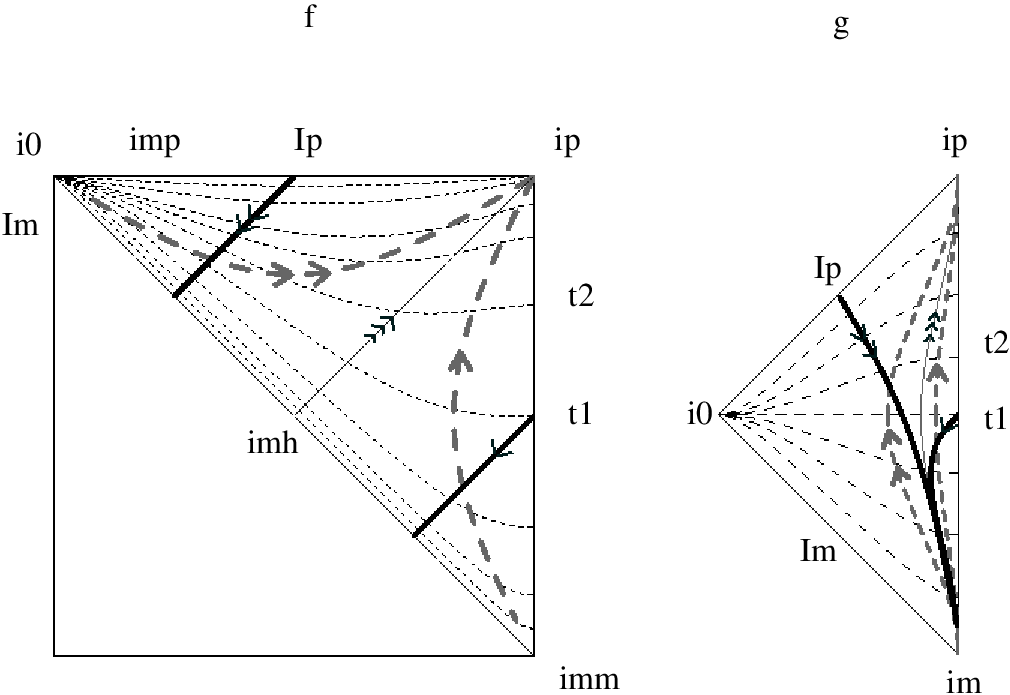
To this end, let us consider the light-cones in the Minkowski metric. Radial null geodesics are simply given by

t=\epsilon r+k

(32)

where $\epsilon=\pm 1$ corresponds to future and past directed null rays respectively. For $\epsilon=0$ we obtain the space-like $t=k$ slices. In order to represent such geodesics in the conformal diagram for metric $f$ , let us first express them in terms of $\tilde{t}$ . For the potentials (29), Eq. (18) reads

\mathrm{d}\tilde{t}=\beta^{-1/2}\mathrm{d}t+{Hr\over 1-H^{2}r^{2}}(\beta-1+H^{2}r^{2})^{1/2}\ \beta^{-1/2}\mathrm{d}r.

(33)

For $\beta=1$ this yields

\tilde{t}=t-r-\frac{1}{2H}\ln\left|{1-Hr\over 1+Hr}\right|.

(34)

The integration constant has been chosen so that $\tilde{t}=t$ at $r=0$ . For $\beta\neq 1$ , Eq. (33) can also be integrated, but the expressions are a bit more cumbersome and we shall omit them in what follows. Note that the change of variables (34) is discontinuous at the de Sitter horizon. This is just as well, since the coordinates ( $\tilde{t},r$ ) become singular at $r\equiv r_{H}=H^{-1}$ , and we need to consider the Kruskal-type coordinates anyway. Substituting in (30) or in (31), we have

U=\Big(\frac{Hr-1}{Hr+1}\Big)e^{-H(t-r)},\quad\quad V=e^{H(t-r)}.

(35)

As noted above, these expressions are valid both for $U\leq 0$ and $U\geq 0$ (with $V>0$ ), and so they cover both quadrants (30) and (31) at once. Now, the radial geodesics are easily given in the $U,V$ chart (as a curve parametrized by $r$ ) by substituting (32) into (35),

U=\Big(\frac{Hr-1}{Hr+1}\Big)e^{-Hk}e^{-H(\epsilon-1)r},\quad\quad V=e^{Hk}e^{H(\epsilon-1)r}.

(36)

Future directed null rays of the Minkowski metric $t=r+k$ , are simply straight lines at 45 degrees,

V=e^{Hk}=const.

On the other hand, past directed null geodesics $\epsilon=-1$ , as well as the spacelike geodesics $\epsilon=0$ , have a rather non-trivial behavior which is illustrated in Fig. 1. For $Hr\ll 1$ , the light-cone emanating from $r=t=0$ (i.e. $k=0$ ) has the same shape as in Minkowski space. However, at $Hr\sim 1$ the past directed light-cone opens up and turns around in the $U,V$ plane. Beyond this turning point, “past directed” null rays of Minkowski start progressing towards the future in the de Sitter diagram! In particular, at large affine parameter, $Hr\to\infty$ , both space-like and past directed null geodesics of Minkowski meet at the upper left corner of the conformal diagram, $U\to+\infty,V\to 0$ , which belongs to the future boundary of de Sitter. In fact, the future timelike infinity $i^{+}$ of Minkowski is mapped into the upper right corner of the de Sitter diagram, the future null infinity ${\cal I}^{+}$ of Minkowski is mapped into the future null infinity of de Sitter (which is spacelike), the spacelike infinity $i^{0}$ and null past infinity ${\cal I}^{-}$ of Minkowski are both mapped to the upper left corner of the de Sitter diagram (see Fig. 2). The situation is more complicated for the past timelike infinity $i^{-}$ of Minkowski. The latter is split into three pieces: a particle moving back in time along a $r=constant$ geodesic of Minkowski space-time would either go to the upper left corner of the de Sitter diagram if $r>r_{H}$ , to the lower right corner if $r<r_{H}$ , or to the $U=0,V=0$ central point if $r=r_{H}$ . However, a given timelike trajectory in Minkowski, stemming from the infinite past ( $t=-\infty,r=r_{H}$ ) can emanate in the de Sitter diagram from any point along the diagonal $V=0$ . The latter diagonal is then representing the whole of the past $r=r_{H}$ infinity of Minkowski. This can be better seen, plotting the null geodesics of de Sitter into a conformal diagram for Minkowski. Inverting (35),

t=r+H^{-1}\ln V,\quad\quad r=\frac{UV+1}{H(1-UV)},

(37)

outgoing (or incoming) null curves are given parametrically in terms of $U$ (or $V$ ) by taking $V=k$ (or $U=k$ ). These are represented in Fig. 2. In particular, one sees that past directed $U=constant$ null lines can intersect the $V=0$ curve anywhere, while they all asymptote the $r=r_{H}$ curve in the Minkowski diagram as $t$ goes to $-\infty$ .

We may then ask whether it is possible to construct a closed time-like curve by combining signals which propagate in the $f$ metric with those propagating in the $g$ metric. We defer this discussion to section 4, where we show that this is not possible for general Type I solutions.

A similar analysis can be performed for other values of $\beta$ . For $\beta>1$ , $D$ is everywhere real and the causal structure is quite similar to the one described above. A minor difference is that the light-cones of Minkowski geodesics are not at 45 degrees near the origin (as they were in Fig. 1). This can be easily seen from Eq. (18). On the other hand, for $\beta<1$ the metric becomes complex in the region $H^{2}r^{2}<1-\beta$ (see Fig. 3).

Let us now consider the issue of global structure. As was stressed above, the coordinates $(r,t)$ cover the full Minkowski space corresponding to the metric $g$ , but only half of the conformal diagram for the extended de Sitter metric, corresponding to $V>0$ (see Fig. 1 (a)). This portion is by itself globally hyperbolic, since the $t=k$ surfaces are Cauchy surfaces for all geodesics of both metrics in this region. However, the region $V>0$ is not geodesically complete, since the null geodesics $U=const.$ of de Sitter reach $V=0$ at finite affine parameter. To obtain a geodesically complete space-time, we can match the solution in the upper half of the conformal diagram with a solution in the lower half of the diagram. For this purpose we introduce a second Minkowski space, with metric $g^{\prime}$ , which will be covered with coordinates $r^{\prime}$ and $t^{\prime}$ . The change of variables (30) and (31) with the substitutions $t\to-t^{\prime}$ , $U\to-U$ , $V\to-V$ , maps the full range of the coordinates $(r^{\prime},t^{\prime})$ into the lower half of the de Sitter conformal diagram, below the diagonal $V=0$ . The full diagram, represented in Fig. 4 and 5, is now geodesically complete. In doing such an extension, we mean we are gluing together one Minkowski spacetime to the other along the past infinity of the $r=r_{H}$ sphere of the former to the future infinity of the $r=r_{H}$ sphere of the latter. These infinities do not belong to the Minkowski spacetimes, but to their boundaries, while they are located in the interior of the de Sitter spacetime. This provides indeed a perfectly fine geometric maximal extension, where all geodesics are complete.

We should add, however, that a maximal extension is usually required to satisfy the equations of motion. The bigravity equations of motion are certainly satisfied everywhere in regions I, II, III and IV of Fig. 4, but it is unclear in which sense they are satisfied along the diagonal $V=0$ . The problem is precisely that we are joining two Minkowski spacetimes [ $(a)$ and $(c)$ of Fig. 4] at a locus which lies at their conformal boundary. It is conceivable that promoting our maximal extension to a solution of the equations of motion might necessitate additional input, such as the inclusion of some source at the time-like infinity of Minkowski. Note further, that there is some arbitrariness in the extensions which are possible, as the already geodesically complete companion can be extended by any other companion to the metric that we are extending. As we have already commented, a similar ambiguity is present in usual General Relativity when a metric must be continued beyond a Cauchy horizon.

The extended diagram, Fig. 4, is not globally hyperbolic. The $t=k$ surfaces of the region $V>0$ are no longer Cauchy surfaces for the whole space-time, since they do not intersect causal geodesics in the lower half of the diagram. A surface which intersects all causal geodesics should cut through both regions, $V>0$ as well as $V<0$ . One such surface is, for instance, the horizontal line $U=V$ . The problem is that, as can be seen in Fig. 4, there are causal geodesics which intersect this surface twice (such as the past directed null rays from $r=t=0$ ). A formal proof that the maximally extended diagram of Fig. 4 is not globally hyperbolic runs as follows. Let us restrict attention to radial geodesics. A Cauchy surface must intersect all causal geodesics once and only once. Let us assume that such a surface $\Sigma$ exists. In particular, $\Sigma$ must intersect the null geodesic $V=0$ of de Sitter space. By continuity, it will also intersect the null geodesics $V=const.$ , in the range $-\delta<V<\delta$ , where $\delta$ is an arbitrarily small positive number. Let us now consider the null geodesic of Minkowski space, parametrized by $r$ in Eq. (36), and let us choose the constant $k<H^{-1}\ln\delta$ . It is clear that the incoming radial geodesic (with $\epsilon=-1$ ) will start at the upper left corner of the de Sitter diagram (at $r\to\infty$ ), and work its way down towards the right boundary of the diagram (at r=0), while $V$ will always remain in the interval $0<V<\delta$ ). Hence, the incoming null geodesic must intersect $\Sigma$ at least once before it reaches $r=0$ . At $r=0$ it bounces and becomes the outgoing null geodesic $V=e^{Hk}<\delta$ , which will intersect $\Sigma$ once more before it reaches null future infinity. Hence, there are geodesics of Minkowski which intersect $\Sigma$ twice, which simply means that this is not a good Cauchy surface for all geodesics in the extended diagram. We will have more to say about the tension between global hyperbolicity and geodesic completeness in section 5.

Let us compare the present situation to that in usual GR. As mentioned above, Cauchy horizons are also present in certain maximally extended solutions of GR, such as Reissner-Nordström or anti-de Sitter space. Whenever there is such a horizon, the equations of motion do not suffice to continue the solution past it, and we need additional input. Usually, analytic continuation is used, or else some boundary conditions at certain time-like boundaries of spacetime are introduced. As mentioned above, in the present context it is not clear whether the equations of motion are satisfied or not at the Cauchy horizon of the maximally extended solution, but this is precisely because this horizon corresponds to a point in the conformal boundary of one of the metrics. In this sense, the situation is no worse than in GR, where we have to prescribe data on certain boundaries in order to determine the maximal extension. Another point to consider is that, physically, Cauchy horizons tend to be unstable to perturbations, because of large blueshift effects expected from the accumulation of perturbations close to the horizon [SP73, CH82]. The same is expected to happen in the present context. Note, e.g., from Fig. 4, that all future directed null geodesics of Minkowski in regions III and IV tend to pile up near the Cauchy horizon at $V=0$ , suggesting that there will be a large backreaction near that surface once we include perturbations.

Another interesting fact of the bi-metric solution is that the concepts of causal past and future are “broadened”, since signals can be transmitted by matter coupled to both metrics. For instance, the observers at $r=0$ , with $V>0$ can see signals emitted by all other observers, and hence they have no future event horizon. Likewise, observers at $r=0$ , with $V<0$ , can emit signals which will eventually reach all other observers, and hence they have no past event horizon. It is tempting to speculate that cosmological bi-gravity solutions, if they can be made sense of, could in principle be relevant to the horizon problem.

2 de Sitter with Schwarzschild

Let us now replace the Minkowski metric by the Schwarzschild one. In this case, the potentials of the Type I solution are given by

\displaystyle p=H^{2}r^{2},\quad\quad q=\frac{2M}{r}.

(38)

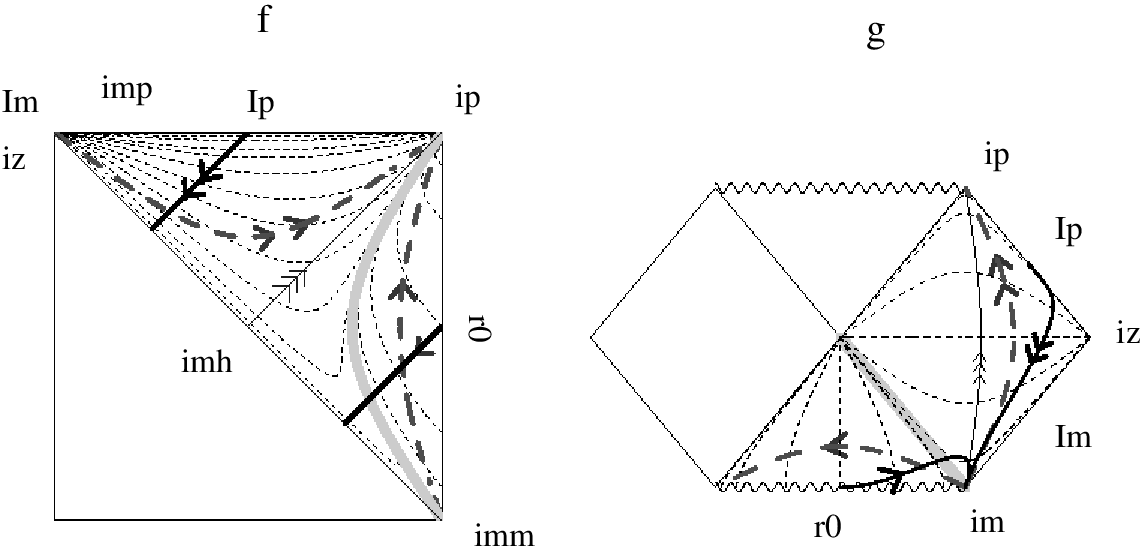
Both metrics have now horizon singularities whenever $p=1$ and $q=1$ , corresponding respectively to $r=r_{H}$ and $r=r_{S}\equiv 2M$ . Those are coordinate singularities from the point of view of each metric considered separately from the other. However, one might be concerned by the possibility to remove such singularities from both metrics at the same time. To study this issue, we first keep $p$ and $q$ unspecified, and note that the coordinate change (18) reads (with $\beta=1$ , which we shall assume in the following)¹²¹² 12 We only discuss here the case $\epsilon_{D}=+1$ , the other case, which corresponds to a change in the sign of time, follows similarly

\mathrm{d}\tilde{t}=\mathrm{d}t-\mathrm{d}r^{*}+\mathrm{d}\tilde{r}^{*},

(40)

$r^{*}$ and $\tilde{r}^{*}$ defining “tortoise” coordinates associated with metric $f$ and $g$ respectively by

	$\displaystyle\mathrm{d}r^{*}$	$\displaystyle=$	$\displaystyle\frac{\mathrm{d}r}{1-q},$		(41)
	$\displaystyle\mathrm{d}\tilde{r}^{*}$	$\displaystyle=$	$\displaystyle\frac{\mathrm{d}r}{1-p}.$		(42)

Thus, introducing the null coordinates $v=t-r^{*},u=t+r^{*}$ for the metric $g$ , and $\tilde{v}=\tilde{t}-\tilde{r}^{*},\tilde{u}=\tilde{t}+\tilde{r}^{*}$ , for the metric $f$ , one has from the above expression (40)

\mathrm{d}\tilde{v}=\mathrm{d}v.

(43)

This means that $v$ is null for both metrics, but also that $(v,r,\theta,\phi)$ are Eddington-Finkelstein coordinates for both metrics. In such a coordinates system none of the metric is singular at the horizons.

Coming back to the explicit expressions for $p$ and $q$ (38) and substituting those in (18) we find

\mathrm{d}\tilde{t}=\frac{1}{\sqrt{\beta}}\left\{\mathrm{d}t+\frac{\sqrt{(H^{2}r^{3}-2M)(H^{2}r^{3}+(\beta-1)r-2\beta M)}}{(r-2M)(1-H^{2}r^{2})}\mathrm{d}r\right\},

(44)

For $\beta=1$ , we have

\tilde{t}=t-r^{*}-\frac{1}{2H}\ln\left|{1-Hr\over 1+Hr}\right|.

(45)

This matches equation (40) where, the Schwarzschild “tortoise” coordinate reads

r^{*}=r+2M\ln|1-r/2M|.

(46)

The analog of Eq. (35) is now

U=\Big(\frac{Hr-1}{Hr+1}\Big)e^{-H(t-r^{*})},\quad\quad V=e^{H(t-r^{*})},

(47)

which, again, is valid both for $U>0$ and $U<0$ (with $V>0$ ), covering both quadrants (30) and (31) of de Sitter, that is to say the region covered by the Eddington-Finkelstein coordinates $(v,r,\theta,\phi)$ . The null and spacelike radial geodesics of Schwarzschild can be written as

t=\epsilon r^{*}+k,

(48)

this being obviously valid in the whole region covered by coordinates $(v,r,\theta,\phi)$ . In the $U,V$ chart these geodesics are given by

U=\Big(\frac{Hr-1}{Hr+1}\Big)e^{-Hk}e^{-H(\epsilon-1)r^{*}},\quad\quad V=e^{Hk}e^{H(\epsilon-1)r^{*}}.

(49)

Again, we find that the null geodesics $t=r^{*}$ correspond to $V=const.$ , (or $v=const$ ) so $V$ is a null coordinate both in Schwarzschild and in de Sitter. The other radial geodesics, with $\epsilon=-1,0$ have a more complicated form, which is qualitatively represented in Fig. 7. Note that for this figure, we have assumed that the Schwarzschild radius $r_{S}$ is smaller that the de Sitter horizon radius $r_{H}$ .

As we discussed previously, and is manifest from Fig. 6, half of the de Sitter diagram (above the diagonal) is mapped onto half of the Schwarzschild diagram (below the diagonal), corresponding to the region mapped by the Eddington-Finkelstein coordinates $(v,r,\theta,\phi)$ . Both half-diagrams are geodesically incomplete, since some geodesics reach the horizons (which dissects the diagrams in two) at finite affine parameter. These geodesics can of course be extended by adding new regions of space-time. If one adds de Sitter and Schwarzschild regions, one obtains a “stair-case” diagram with an infinite chain of de Sitter and Schwarzschild space-times, two adjacent de Sitter (resp. Schwarzschild) space-times being linked together by a common Schwarzschild (resp. de Sitter) space-time. Needless to say, there is also a tension in this case between geodesic completeness and global hyperbolicity, as we found in the Minkowski-de Sitter case.

As we will discuss, this applies to more general situations where one of the metrics has a horizon which is not shared by the other one. As noted previously, the new metric (new “step”) which can be added to the stair does not necessarily correspond to the same solution as the one of the last step of the stair, since one of the two metrics does not determine uniquely the form of the other. Thus, in general we can construct “stair-case” diagrams with steps having different forms. Note further, that in the case considered here, the stairs can always be finished by adding a Minkowski spacetime, linked to a Schwarzschild space-time along a sphere of radius $r_{H}$ at time-like infinity.

3 de Sitter with de Sitter

When both metrics are de Sitter, the potentials are given by

p=H_{1}^{2}r^{2}\quad\quad q=H^{2}_{2}r^{2}.

(50)

For $\beta=1$ , the analysis proceeds along the same lines as in the previous subsection, with the only difference that the (de Sitter) tortoise coordinate is now given by

r^{*}=-{1\over 2H_{2}}\ln\left|{1-H_{2}r\over 1+H_{2}r}\right|.

(51)

The corresponding causal diagram is represented in Fig. 9

Aside from the choice $\beta=1$ , the de Sitter with de Sitter solution allows for another way of having $D^{2}>0$ for the entire range of $r$ . Indeed, it is enough to have $H_{1}^{2}\geq\beta H_{2}^{2}$ and $\beta\geq 1$ or $H_{1}^{2}\leq\beta H_{2}^{2}$ and $\beta\leq 1$ . Choosing for example $\beta$ given by

\beta={H_{1}^{2}\over H_{2}^{2}},

(52)

we have

H_{1}\tilde{t}=H_{2}t-\frac{1}{2}\ln\left|1-H_{1}^{2}r^{2}\over 1-H_{2}^{2}r^{2}\right|,

(53)

or $H_{1}(\tilde{t}-\tilde{r}^{*})+\ln(1+H_{1}r)=H_{2}(t-r^{*})+\ln(1+H_{2}r)$ . Thus, the Kruskal coordinates (30-31) for the metric $p$ can be expressed in terms of coordinates $t$ and $r$ as

U=\left(\frac{H_{1}r-1}{H_{2}r+1}\right)e^{-H_{2}(t-r^{*})},\quad\quad V=\left({H_{2}r+1\over H_{1}r+1}\right)e^{+H_{2}(t-r^{*})},

(54)

where $r^{*}$ is given by (51). The corresponding diagram is given in Fig. 10.

4 Closed time-like curves?

An interesting question regarding the bigravity solutions is whether we can construct closed time-like curves (CTC) or closed causal curves (CCC) by patching together future directed geodesics corresponding to both metrics. The existence of these curves is seen as a serious pathology of a solution and they are forbidden by the chronology protection conjecture which basically states that quantum effects and vacuum polarization effects prevent the formation of CCC, as this curves lead to instabilities due to the piling of modes [BMV07].

For $\beta=1$ it is easy to show that CTC cannot be constructed by using the “tortoise” coordinates $r^{*}$ and $\tilde{r}^{*}$ that we defined in equations (41) and (42), as well as the null (for both metric) coordinate $v$ (in all this subsection, we keep the functions $p$ and $q$ unspecified). The radial null and time-like geodesics of both metrics are given by

t=\epsilon r^{*}+k,\quad\quad\tilde{t}=\tilde{\epsilon}\tilde{r}^{*}+\tilde{k},

(Here $\epsilon=\pm 1,0$ for outgoing and incoming null rays, or for spacelike geodesics, respectively, and similarly for $\tilde{\epsilon}$ ). Thus, any future directed causal curve with respect to $f$ or $g$ has the property that $\mathrm{d}v\geq 0$ , and $\mathrm{d}v$ vanishes only along the outgoing null radial geodesic. Once $v$ increases, even if it is by just a little bit, it is impossible to go back to the original value by following a future directed time-like curve, which means that such curve cannot be closed.

Here, we disregard the possibility of making global identifications in the coordinate $v$ , which might allow for the construction of a closed loop. Of course, even in flat space with a single metric, closed time-like curves could be constructed by global identifications, and in what follows we shall ignore this somewhat artificial setup. We shall only be concerned with the possibility of locally constructing closed time-like curves within a given coordinate patch of space-time, without identifications.

To analyse the general case $\beta\neq 1$ it is convenient to separately consider the following regions of space-time:

a: For $(1-p)<0$ , and $(1-q)<0$ the condition $\mathrm{d}r=0$ defines a space-like surface for both metrics $f$ and $g$ . This means that $r$ can only change monotonically along time-like curves of both metrics, making it impossible to close them in this region.

b: For $(1-p)<0$ and $(1-q)>0$ , the condition $\mathrm{d}t=0$ defines a space-like surface for the metric $g$ . Also, from (18) with $\mathrm{d}t=0$ , we have

\left|{\mathrm{d}\tilde{t}\over\mathrm{d}\tilde{r}^{*}}\right|^{2}=1+{1\over\beta}\left({1-p\over 1-q}\right)^{2}-{\beta+1\over\beta}\left({1-p\over 1-q}\right)>1.

(55)

Since $\tilde{t}$ is space-like in metric $f$ this means that the surface $\mathrm{d}t=0$ [which is also defined by Eq. (55)] is space-like in metric $f$ too. Hence, $t$ changes monotonically along time-like curves of both $f$ and $g$ , and as a consequence such curves cannot be closed.

c: If $(1-p)>0$ and $(1-q)<0$ , then the surface $\mathrm{d}\tilde{t}=0$ is space-like for $f$ . From (18) with $\mathrm{d}\tilde{t}=0$ , we have

\left|{\mathrm{d}t\over\mathrm{d}r^{*}}\right|^{2}=1+\beta\left({1-q\over 1-p}\right)^{2}-(\beta+1)\left({1-q\over 1-p}\right)>1.

(56)

Since $t$ is space-like in metric $g$ , Eq. (56) means that the surface $\mathrm{d}\tilde{t}=0$ is space-like in metric $g$ too, and $\tilde{t}$ must be monotonic on time-like curves, which therefore cannot close.

d: Finally, if $(1-p)>0$ and $(1-q)>0$ , then we must distinguish two cases. For $p\geq q$ , it is easy to see that $A>0$ in Eq. (12), and therefore $\mathrm{d}t=0$ is space-like for both metrics $f$ and $g$ . Hence, $t$ is monotonic for time-like curves of both metrics. On the other hand, for $p\leq q$ , Eq. (56) for $\mathrm{d}\tilde{t}=0$ leads to

\left|{\mathrm{d}t\over\mathrm{d}r^{*}}\right|^{2}<1.

(57)

Since now $t$ is time-like in metric $g$ , this means that $\mathrm{d}\tilde{t}=0$ is a space-like surface for this metric. Of course $\mathrm{d}\tilde{t}=0$ is also space-like for $f$ , and so $\tilde{t}$ is monotonic along causal curves for both metrics.

This completes the proof for the individual regions listed above. It is remarkable that in spite of the strong differences in the light-cone structure of both metrics, it is not possible to draw closed time-like curves in any of the regions. The reason is that the future light-cone for one of the metrics never contains a part of the past light-cone for the other metric. Thus, we can always find a coordinate which labels hypersurfaces which are space-like for both metrics. This coordinate must grow monotonically along time-like curves.

By continuity, at the boundaries in between the regions, the future light-cone of one of the metrics can at most touch the past light-cone of the other metric, sharing perhaps a common null direction for both metrics. Even if this were the case, a future directed time-like geodesic with respect to one of the metrics can never get to the inside of the past light cone with respect to the other metric, and closed time-like curves cannot be constructed even if we cross the boundaries between the individual regions¹³¹³ 13 In the examples we have examined, the situation where the future light-cone of one of the metrics marginally touches the past light-cone of the other metric at the boundary between regions does not arise. If it did, then there might be closed future-directed null curves at such boundary. Note, however, that since the boundary is at $r=const.$ , this situation can only happen when both metrics have a common event horizon at the same value of $r$ . The possibility of having closed null curves on these boundaries may require a case by case analysis, and is left for further research..

5 Global Hyperbolicity vs. Geodesic Completeness

In section 1, we showed that global hyperbolicity may be lost when a solution of bigravity is maximally extended to obtain a geodesically complete metric (not necessarily a solution of the equations of motion).

The main idea of the proof can be easily generalized to other situations¹⁴¹⁴ 14 We will use the notation and conventions of [HE73]. A subindex $f$ or $g$ will indicate that the concept refers to the metric $f$ or $g$ respectively. (see Fig. 11 to get an intuitive idea). Let us consider a time orientable manifold ${\mathcal{M}}$ endowed with two globally hyperbolic metrics $f$ and $g$ . Let us suppose that there exists a point $p$ in the boundary of the manifold ( $p\in\overline{{\mathcal{M}}}$ ) through which the manifold can be extended for the metric $g$ through the past (future). Any Cauchy surface $\Sigma$ for the metric $g$ will have to intersect the causal future or causal past of $p$ , $J_{g}(p)$ . If for any such a surface there is a non-causal curve for $g$ which intersects $\Sigma$ more than once and which is timelike for $f$ , $\Sigma$ will not be a Cauchy surface for $f$ .

Let us see with some examples that the existence of this curve $\gamma$ for any Cauchy surface $\Sigma$ is a generic feature when one extends the non-geodesically complete manifold through a horizon which is not shared by both metrics or when both metrics share a horizon but it is of different type for each of them.

First, take the future null cone for the metric $g$ at a point $p$ of the boundary of a manifold ${\mathcal{M}}$ , i.e., $p\in\overline{\mathcal{M}}$ . If $\overline{\mathcal{M}}$ is b-complete¹⁵¹⁵ 15 A manifold $\mathcal{M}$ endowed with a metric $g$ is b-complete if there is an endpoint for every continuous curve of finite length as measured by a generalized affine parameter [HE73]., the light rays in the null cone can be approached by both connected timelike and connected spacelike curves in all the disconnected parts in which $\overline{\mathcal{M}}$ is divided by the cone. When the manifold is maximally extended for $g$ through the past at $p$ the future lightcone $T^{+g}_{p}$ can be approached by spacelike curves $\{\gamma_{n}\}\in\mathcal{M}$ (see Fig 11). This means that they must converge to a curve $\gamma_{g}$ in $\overline{{\mathcal{M}}}_{g}$ and similarly to a curve $\gamma_{f}$ in $\overline{{\mathcal{M}}}_{f}$ ¹⁶¹⁶ 16 The map from one of this limit curves to the other one is not necessarily continuous as the topology of $\overline{{\mathcal{M}}}$ depends on the metric which is used to make the conformal compactification.. For the $g$ metric, this curve is composed of two future directed null curves stemming from $p$ , and thus every Cauchy surface $\Sigma$ will have to intersect both curves in $J_{g}^{+}(p)$ or $J_{g}^{-}(p)$ or at $p$ . Let us suppose that it intersects $J_{g}^{+}(p)$ . As the surface $\Sigma$ must be spacelike for both $f$ and $g$ , there exists $m\in\mathbb{N}$ such that it will also intersect twice the curves $\gamma_{n}$ for $n\geq m$ . The curve $\gamma_{f}\cap{\mathcal{M}}$ will be null as for the $g$ metric. If it is timelike for the $f$ metric so will be the curves $\gamma_{n}$ for $n\geq q$ for a certain $q\in\mathbb{N}$ . Now consider a curve $\gamma\in\mathcal{M}$ in $\{\gamma_{n}\}$ for $n\geq\mathrm{max}(q,m)$ . This will be a timelike curve for $f$ which intersects twice $\Sigma$ , which will not be an appropriate Cauchy surface.

In more abstract terms, the curve $\gamma$ can be characterized as follows. Let us consider a family $\lambda_{p}$ of future (past) directed non-spacelike curves for the $g$ metric stemming from $p\in\overline{\mathcal{M}}$ . Given a non-causal curve for $g$ in the future domain of dependence of $\lambda_{p}$ , $\gamma\in\mathrm{int}\left(D_{g}^{+}(\lambda_{p},{\mathcal{M}})\right)$ , such that $\gamma$ is non-compact and without boundary in the open set $\mathrm{int}\left(D_{g}^{+}(\lambda_{p},{\mathcal{M}})\cap D^{-}_{g}(\Sigma)\right)$ but it is compact in $D_{g}^{+}(\lambda_{p},{\mathcal{M}})\cap D^{-}_{g}(\Sigma)$ , if $\gamma\cap D^{-}_{g}(\Sigma)$ is timelike for the companion $f$ metric, this will be such a curve. To see it, it is enough to realize that being timelike for $f$ which is globally hyperbolic, $\gamma$ can not be a self intersecting curve. Thus, being compact and not-self intersecting, $\gamma$ will have two boundary points $q_{1}$ and $q_{2}$ in $D_{g}^{+}(\lambda_{p},{\mathcal{M}})\cap D^{-}_{g}(\Sigma)$ (which may coincide). As $\gamma\cap\dot{D}^{+}(\lambda_{p},{\mathcal{M}})={\O}$ and $\gamma$ is non compact and without boundary in $\mathrm{int}\left(D_{g}^{+}(\lambda_{p},{\mathcal{M}})\cap D^{-}_{g}(\Sigma)\right)$ , these points can only be in $\Sigma$ . Thus, the curve intersects the Cauchy surface at least twice.

It is not hard to identify other pathological situations where global hyperbolicity is lost once bigravity solutions are extended (see e.g. [Bla07b]). They refer to particular situations and we shall not elaborate on them.

Chapter 7 Perturbations around Bigravity Solutions

In the previous Chapter we have considered a non-linear extension of massive gravity consisting of two interacting metrics that at the linear level reduce to certain models of massive gravity. Here we will study the linear regime of perturbations to some of the solutions more closely. We will be interested in two cases. First, there are some Type I solutions that reduce to two diagonal flat metrics which are not proportional to each other. This bi-flat solution is very interesting as Lorentz invariance is broken in the vacuum. This will give rise to mass terms which do not suffer from neither vDVZ discontinuity and strong coupling nor ghost states [RT08, Rub04]. As we will see, the dispersion relations are also modified in this set-up (there are two “speeds of light”). This solution is also interesting because it corresponds to the field far from the sources in a wider class of spherically symmetric exact solutions of the Schwarzschild form.

Besides, even when both metrics are proportional, the mass term of the perturbations for a generic potential $V[\{\tau_{n}\}]$ is not FP. For Minkowski spacetime this means that only the case where the FP condition is satisfied can be considered as a stable vacuum of the theory. For other mass terms, a Lorentz breaking cut-off is necessary to regularize the decay rate [CJM04]. As the cut-off must be of the order of the mass scale, the theory is effectively equivalent to GR within its range of validity. For non-trivial backgrounds the appearance of a curvature scale suggests the possibility of a softer cut-off which would allow more general mass terms. We will study this possibility in the second part of this Chapter and find that this possibility does not happen for bi-de Sitter solutions. Finally, we will study the case of two de Sitter solutions with a common $SO(3)$ invariance. This Chapter is based on [BDG07] (see also [Bla07b, Bla06]). A potentially interesting possibility which we leave for future research is a background with a black hole for one of the metrics [Bla]. Black holes are not yet well understood in the theories of massive gravity and bigravity provides a simple scenario to study some of their features (see also [DTZ07] for the ghost condensate case and [JW08] for some problems of black holes when Lorentz invariance is broken). Besides, it is well known that in GR stationary black holes can not carry massive tensor field (no hair theorem [Bek72]). It would be interesting to study whether it can support a non-covariant massive tensor hair.

1 Perturbations around Lorentz-breaking bi-flat metrics

In a theory with two metrics with Einstein-Hilbert kinetic terms and no interaction, there are 4+4 ADM Lagrange multipliers¹¹ 1 For the ADM analysis of massive gravity see [BD72, DR05, GG05a].. When we add a non-derivative interaction which preserves diagonal diffeomorphisms, only 4 combinations of these may in principle appear non-linearly in the action [DK02]. For these, their equation of motion relates them to the other variables, but they do not lead to further constraints. Thus, we have a minimum of 4 and a maximum of 8 Lagrange multipliers for 20 metric components. Hence, we generically expect a maximum of $(10-4)+(10-8)=6+2=8$ degrees of freedom and a minimum of $(10-8)\times 2=2+2=4$ . In a Lorentz-invariant context, the first possibility corresponds to a massless and a massive graviton, whereas the second would correspond to two massless gravitons. In the Lorentz breaking context, it is possible to have a massive graviton with just two physical polarizations [DTT05b, GG05a].

Let us consider a general potential $V[\{\tau_{n}\}]$ as in (2). As we showed in the previous Chapter, the vacuum energies $\rho_{f}$ and $\rho_{g}$ can be tuned so that the previous potential has asymptotically bi-flat solutions. At large distances from the origin, these take the form

\displaystyle g_{\mu\nu}=\eta_{\mu\nu},\quad f_{\mu\nu}=\gamma\tilde{\eta}_{\mu\nu},

(1)

where

\tilde{\eta}_{\mu\nu}=\eta_{\mu\nu}-\frac{\beta-1}{\beta}\delta_{\mu}^{0}\delta_{\nu}^{0},

(2)

and $\eta_{\mu\nu}=\mathrm{diag}(1,-1,-1,-1)$ . The parameters $\gamma$ and $\beta$ are related by Eq. (15). For $\beta\neq 1$ , we cannot simultaneously write both metrics in the canonical form $\eta_{\mu\nu}$ , and Lorentz invariance breaks down to spatial rotations²² 2 For $\beta=1$ , we have proportional flat metrics the perturbations of which can be obtained from the flat space-time limit of the calculations done in the next section.. It will be convenient to introduce the general perturbation in the form

	$\displaystyle f^{\mu\nu}$	$\displaystyle=$	$\displaystyle\gamma^{-1}\big(\tilde{\eta}^{\mu\nu}+h_{f}^{\phantom{f}\mu\nu}\big),$		(3)
	$\displaystyle g_{\mu\nu}$	$\displaystyle=$	$\displaystyle\eta_{\mu\nu}+h^{g}_{\phantom{f}\mu\nu},$		(4)

where $\tilde{\eta}^{\mu\nu}$ is the inverse of $\tilde{\eta}_{\mu\nu}$ . The perturbation to the metric $f$ has been defined with the upper indices, just because this simplifies the manipulations which yield the action quadratic in the perturbations shown below. For the remainder of this section, all space-time indices will be raised and lowered with the canonical Minkowski metric $\eta_{\mu\nu}$ . The interaction Lagrangian quadratic in perturbations then reads

$\displaystyle\tilde{L}_{int}$	$\displaystyle\equiv$	$\displaystyle L_{int}-\sqrt{-g}\rho_{g}-\sqrt{-f}\rho_{f}=$	(5)
		$\displaystyle-\frac{M^{4}}{8}\Big\{n_{2}(h^{g}_{\phantom{f}ij}+h_{f}^{\phantom{f}ij})(h^{g}_{\phantom{f}ij}+h_{f}^{\phantom{f}ij})+n_{0}(h^{g}_{\phantom{f}00}+\beta^{-1}h_{f}^{\phantom{f}00})(h^{g}_{\phantom{f}00}+\beta^{-1}h_{f}^{\phantom{f}00})$
		$\displaystyle-2n_{4}(h^{g}_{\phantom{f}00}+\beta^{-1}h_{f}^{\phantom{f}00})(h^{g}_{\phantom{f}ii}+h_{f}^{\phantom{f}ii})+n_{3}(h^{g}_{\phantom{f}ii}+h_{f}^{\phantom{f}ii})^{2}\Big\},$

where, after imposing (15),

$\displaystyle M^{4}$	$\displaystyle=$	$\displaystyle 4\zeta\left(\frac{\gamma^{4}}{\beta}\right)^{v},\quad n_{0}=3n_{3}-2n_{4}-n_{2}+\gamma\frac{\partial}{\partial\gamma}\left(\sum_{n}n\gamma^{-n}(-1+\beta^{n})V_{0}^{(n)}\right),$
$\displaystyle n_{2}$	$\displaystyle=$	$\displaystyle-\sum n^{2}\gamma^{-n}V_{0}^{(n)},\quad n_{3}=uvV_{0}+\sum_{n}n[v-u]\gamma^{-n}V^{(n)}_{0}-\sum_{m,n}nm\gamma^{-(n+m)}V_{0}^{(n,m)},$
$\displaystyle n_{4}$	$\displaystyle=$	$\displaystyle n_{0}+\beta\frac{\partial}{\partial\beta}\left(\sum_{n}n\gamma^{-n}(-1+\beta^{n})V_{0}^{(n)}\right).$	(6)

For the sake of simplicity, we will restrict to potentials $V[\{\tau_{n}\}]$ for which Eq. (15) is independent³³ 3 The case where (15) is satisfied independently of $\beta$ and $\gamma$ leads to the condition $3n_{3}-3n_{0}-n_{4}=0,\quad n_{4}=n_{0},$ (7) which, as we shall see, corresponds to the case of no corrections to the Newton’s law. An example of an interaction where these conditions are satisfied is a potential which is only a function of the ratio of determinants of $f$ and $g$ ; that is $V\left[\{\tau_{n}\}\right]=V[f/g]$ . In this particular case, there is an enhanced symmetry under independent “non-diagonal” transverse diffeomorphisms, which do not change the value of the determinants of the respective metrics. of $\beta$ , and determines $\gamma$ . From equation (6), this implies $n_{0}=n_{4}$ . In particular, this class includes the interaction (23), which, as we shall see, leads to a rather pathological behaviour for the perturbations. On the other hand, it is general enough to be representative of generic choices of potentials.

In the works [Rub04, Dub04] the case of a single graviton with a Lorentz violating mass term has been discussed. For comparison with those references, it will be useful to introduce

m_{0}^{2}=-cn_{0},\ m_{1}^{2}=0,\ m_{2}^{2}=cn_{2},\ m_{3}^{2}=-cn_{3},\ m_{4}^{2}=-cn_{4},

where $c>0$ is an irrelevant constant which has the dimensions of mass squared.

Note that the components $h^{g}_{\phantom{f}0i}$ and $h_{f}^{\phantom{f}0i}$ are absent from (5). As noted in [BCNP07] the absence of such terms is a consequence of invariance under diagonal diffeomorphisms in this background (see below). In the case of a single graviton (with a Fierz-Pauli kinetic term), the absence of $h_{0i}$ in the mass term leads to a very interesting behaviour [Dub04, DTT05b, DTT05a], where the two polarizations of the massless graviton acquire mass, while all the other modes do not propagate⁴⁴ 4 It should be stressed that the absence of $0i$ components is a peculiarity of the background considered. By suitable adjustment of the vacuum energies, the theory we are considering also admits the Lorentz preserving vacuum of type II, where $f_{\mu\nu}=g_{\mu\nu}=\eta_{\mu\nu}$ . In that case, the interaction term leads to the Fierz-Pauli mass term for a combination of the two gravitons. This mass term does contain the $0i$ components..

Let us now investigate whether a similar phenomenon occurs in our model. The situation is not directly reducible to that of a single graviton, since the equations of motion are not diagonal. Also, the kinetic term breaks the Lorentz invariance. It is convenient to decompose the perturbations into irreducible representations of the spatial rotations,

$\displaystyle h^{X}_{\phantom{f}00}$	$\displaystyle=$	$\displaystyle 2A^{X},$
$\displaystyle h^{X}_{\phantom{f}0i}$	$\displaystyle=$	$\displaystyle B^{X}_{,i}+V^{X}_{i},$
$\displaystyle h^{X}_{\phantom{f}ij}$	$\displaystyle=$	$\displaystyle 2\psi^{X}\delta_{ij}-2E^{X}_{,ij}-2F^{X}_{(i,j)}-t_{ij}^{X},$	(8)

where $t^{X}_{\phantom{X}ii}=t^{X}_{\phantom{X}ij,i}=V^{X}_{\phantom{X}i,i}=F^{X}_{\phantom{X}i,i}=0$ for $X=f,g$ , and all space-time indices are raised and lowered with the metric $\eta_{\mu\nu}$ .

To second order in the perturbations, the kinetic terms in (1) can be written in terms of these scalar, vector and tensor variables as:

$\displaystyle L_{K}$	$\displaystyle=$	$\displaystyle\frac{1}{2\kappa_{g}}\Big\{-\frac{1}{4}t^{g}_{ij}\Box t^{g}_{ij}-\frac{1}{2}\left(V_{i}^{g}+\dot{F}_{i}^{g}\right)\Delta\left(V^{g}_{i}+\dot{F}^{g}_{i}\right)+4\Delta\psi^{g}\left(A^{g}-\dot{B}^{g}-\ddot{E}^{g}\right)$	(9)
		$\displaystyle-2\psi^{g}\Delta\psi^{g}-6(\dot{\psi}^{g})^{2}\Big\}+\frac{1}{2\tilde{\kappa}_{f}}\Big\{-\frac{1}{4}t^{f}_{ij}\tilde{\Box}t^{f}_{ij}-\frac{\beta^{-1}}{2}\left(V^{f}_{i}+\beta\dot{F}^{f}_{i}\right)\Delta\left(V^{f}_{i}+\beta\dot{F}^{f}_{i}\right)$
		$\displaystyle\hskip 28.45274pt+4\beta^{-1}\Delta\psi^{f}\left(A^{f}-\beta\dot{B}^{f}-\beta^{2}\ddot{E}^{f}\right)-2\psi^{f}\Delta\psi^{f}-6\beta(\dot{\psi}^{f})^{2}\Big\},$

where $\tilde{\Box}=\tilde{\eta}^{\mu\nu}\partial_{\mu}\partial_{\nu}$ , $\tilde{\kappa}_{f}=\gamma^{-1}\beta^{1/2}\kappa_{f}$ and dot means a derivative with respect to time. At the linear level, the transformations generated by independent diffeomorphisms $\delta x^{\mu}=\xi^{\mu}_{X}$ in each one of the metrics can be expressed as

\displaystyle\delta h^{g}_{\phantom{g}\mu\nu}=2\partial_{(\mu}\xi^{g}_{\nu)},\quad\delta h^{f}_{\phantom{g}\mu\nu}=2\eta_{\beta(\mu|}\tilde{\eta}^{\alpha\beta}\partial_{\alpha}\xi^{f}_{|\nu)}.

(10)

Note that the kinetic term is written in terms of the following quantities:

	$\displaystyle t_{ij}^{g},\ V_{i}^{g}+\dot{F}_{i}^{g},\ \psi,\ A^{g}-\dot{B}^{g}-\ddot{E}^{g},$
	$\displaystyle t_{ij}^{f},\ V_{i}^{f}+\beta\dot{F}_{i}^{f},\ \psi,\ A^{f}-\beta\dot{B}^{f}-\beta^{2}\ddot{E}^{f},$		(11)

which are invariant under both gauge transformations. On the other hand, the full action (including the mass terms), is invariant only under the diagonal gauge invariance

\xi_{\mu}^{g}=\xi^{f}_{\mu}.

(12)

No second order scalar combination of $h^{X}_{\phantom{X}0i}$ is invariant under this gauge invariance, which implies that those terms are always absent (cf. (5)). We may now analyze the propagating degrees of freedom.

1 Tensor Modes

The linearized Lagrangian for the tensor and vector modes can be expressed as

$\displaystyle L_{t,v}$	$\displaystyle=$	$\displaystyle\frac{1}{2\kappa_{g}}\Big\{-\frac{1}{4}t^{g}_{ij}\Box t^{g}_{ij}-\frac{1}{2}\left(V_{i}^{g}+\dot{F}_{i}^{g}\right)\Delta\left(V^{g}_{i}+\dot{F}^{g}_{i}\right)\Big\}$	(13)
		$\displaystyle+\frac{1}{2\tilde{\kappa}_{f}}\Big\{-\frac{1}{4}t^{f}_{ij}\tilde{\Box}t^{f}_{ij}-\frac{\beta^{-1}}{2}\left(V^{f}_{i}+\beta\dot{F}^{f}_{i}\right)\Delta\left(V^{f}_{i}+\beta\dot{F}^{f}_{i}\right)\Big\}$
		$\displaystyle-\frac{M^{4}}{8}\Big\{n_{2}(t_{ij}^{g}+t_{ij}^{f})^{2}-2n_{2}(F_{i}^{g}+F_{i}^{f})\Delta(F_{i}^{g}+F_{i}^{f})\Big\},$

where $\tilde{\kappa}_{f}=\gamma^{-1}\beta^{1/2}\kappa_{f}$ . The corresponding equations of motion in Fourier space read

	$\displaystyle\omega^{2}t_{ij}^{g}$	$\displaystyle=$	$\displaystyle{\bf k}^{2}t_{ij}^{g}+\kappa_{g}M^{4}n_{2}(t_{ij}^{g}+t_{ij}^{f}),$		(14)
	$\displaystyle\beta\omega^{2}t_{ij}^{f}$	$\displaystyle=$	$\displaystyle{\bf k}^{2}t_{ij}^{f}+\tilde{\kappa}_{f}M^{4}n_{2}(t_{ij}^{g}+t_{ij}^{f}),$		(15)

from which we obtain the dispersion relations

\omega^{2}_{\pm}=\frac{1}{2\beta}\Big((\beta+1){\bf k}^{2}+\kappa_{0}M^{4}\pm\sqrt{((\beta+1){\bf k}^{2}+\kappa_{0}M^{4})^{2}-4\beta{\bf k}^{2}(\kappa_{1}M^{4}+{\bf k}^{2})}\Big),

(16)

where $\kappa_{0}=n_{2}(\beta\kappa_{g}+\tilde{\kappa}_{f})$ and $\kappa_{1}=n_{2}(\kappa_{g}+\tilde{\kappa}_{f})$ .

At high energies, we have

\omega^{2}_{+}\approx{\bf k}^{2},\quad\omega^{2}_{-}\approx{\beta}^{-1}{\bf k}^{2}.

(17)

In this limit, each one of the two gravitons propagates in its own metric (with the corresponding ‘‘speed of light”⁵⁵ 5 Superluminal propagation has previously been considered in several contexts (see e.g. [BMV06, BMV07] for a recent discussion). Clearly, such propagation cannot by itself be considered pathological. Indeed, in the present case we always have superluminal propagation from the point of view of one of the metrics, whereas there is not any superluminal propagation from the point of view of the other metric. Nevertheless, as we have seen in the previous Chapter, the global structure of non-linear bi-gravity solutions is complicated in general, and its interpretation is far from trivial. Even more, instantaneous interaction is also present in certain theories of Lorentz breaking massive gravity [Beb08].) along null directions $k^{\mu}=(\omega,{\bf k})$ satisfying

g^{\mu\nu}_{X}k_{\mu}k_{\nu}\approx 0.

The low energy expansion of (16) is given by

	$\displaystyle\omega^{2}_{-}$	$\displaystyle=$	$\displaystyle\frac{\kappa_{1}}{\kappa_{0}}{\bf k}^{2}+O({\bf k}^{4}),$		(18)
	$\displaystyle\omega^{2}_{+}$	$\displaystyle=$	$\displaystyle\frac{\kappa_{0}M^{4}}{\beta}+\left({\tilde{\kappa}_{f}+\beta^{2}\kappa_{g}\over\beta\tilde{\kappa}_{f}+\beta^{2}\kappa_{g}}\right){\bf k}^{2}+O({\bf k}^{4}).$		(19)

The first dispersion relation corresponds to two massless polarizations which propagate at the “intermediate” speed

c_{s}^{2}={\omega_{-}^{2}\over{\bf k}^{2}}={\kappa_{1}\over\kappa_{0}}={\kappa_{g}+\tilde{\kappa}_{f}\over\beta\kappa_{g}+\tilde{\kappa}_{f}}.

Note that for $\beta>1$ we have $\beta^{-1}<c_{s}^{2}<1$ , while for $\beta<1$ we have $1<c_{s}^{2}<\beta^{-1}$ . The second dispersion relation, Eq. (19), corresponds to two massive polarizations. It is easy to check that the graviton polarizations are stable and tachyon free as long as $\kappa_{0}>0$ , in the whole range of momenta ${\bf k}$ . The second dispersion relation (19) corresponds to the massive graviton.

2 Vector Modes

From the Lagrangian (13), we find that $V_{i}^{g}$ and $V_{i}^{f}$ do not appear in the interaction term. Varying with respect to the vector fields we have,

$\displaystyle\Delta(V_{i}^{g}+\dot{F}_{i}^{g})$	$\displaystyle=$	$\displaystyle 0,$	(20)
$\displaystyle\Delta\left(\dot{V}^{g}_{i}+\ddot{F}^{g}_{i}\right)$	$\displaystyle=$	$\displaystyle-M^{4}n_{2}\kappa_{g}\Delta\left(F^{g}_{i}+F^{f}_{i}\right),$	(21)
$\displaystyle\Delta(V_{i}^{f}+\beta\dot{F}_{i}^{f})$	$\displaystyle=$	$\displaystyle 0,$	(22)
$\displaystyle\Delta\left(\dot{V}^{f}_{i}+\beta\ddot{F}^{f}_{i}\right)$	$\displaystyle=$	$\displaystyle-M^{4}n_{2}\tilde{\kappa}_{f}\Delta\left(F^{g}_{i}+F^{f}_{i}\right).$	(23)

We can always use the diagonal diffeomorphism invariance to work in the gauge where $V_{i}^{g}=0$ . It then follows from (20) that $F_{i}^{g}=F_{i}(\vec{x})+f_{i}^{g}(t)$ , where $F_{i}$ are arbitrary functions of position and $f_{i}$ are arbitrary functions of time. The latter are in fact irrelevant, because $F_{i}^{X}$ enters the metric only through spatial derivatives. Formally, we may describe this as a gauge invariance $F_{i}^{X}\mapsto F_{i}^{X}+f_{i}^{X}(t)$ , which we can use in order to write, without loss of generality,

F_{i}^{g}=F_{i}(\vec{x}).

It then follows from (21) that

F_{i}^{f}=-F_{i}(\vec{x}),

where again we eliminate the additive time dependent part. Finally, from (22) we obtain

V_{i}^{f}=\tilde{f}_{i}(t),

where $\tilde{f}_{i}$ are new arbitrary functions of time. This is not a desirable situation, since it means that the initial conditions do not determine the future evolution of $V_{i}^{f}$ . Technically, the absence of the fields $V_{i}^{g}$ and $V_{i}^{f}$ in the mass term leads to an enhanced gauge invariance in the linearized Lagrangian. Indeed, we can consider independent gauge transformations for each of the metrics

h_{\mu\nu}\mapsto h_{\mu\nu}+2\partial_{(\mu}\xi^{h}_{\nu)},\quad l_{\mu\nu}\mapsto l_{\mu\nu}+2\partial_{(\mu}\xi^{l}_{\nu)},

(24)

of the form $\xi_{i}^{X}=\xi_{i}^{X}(t)$ . As we have discussed, these do not affect the $F_{i}^{X}$ , but can be used to give both of the $V_{i}^{X}$ an arbitrary time dependence.

3 Scalar Modes

The Lagrangian for the scalar modes can be expressed as

$\displaystyle L_{s}$	$\displaystyle=$	$\displaystyle\frac{1}{\kappa_{g}}\Big\{2\Delta\psi^{g}\left(A^{g}-\dot{B}^{g}-\ddot{E}^{g}\right)-\psi^{g}\Delta\psi^{g}-3(\dot{\psi}^{g})^{2}\Big\}$
		$\displaystyle+\frac{1}{\tilde{\kappa}_{f}}\Big\{2\beta^{-1}\Delta\psi^{f}\left(A^{f}-\beta\dot{B}^{f}-\beta^{2}\ddot{E}^{f}\right)-\psi^{f}\Delta\psi^{f}-3\beta(\dot{\psi}^{f})^{2}\Big\}$
		$\displaystyle-\frac{M^{4}}{2}\Big\{n_{2}\{3(\psi^{g}+\psi^{f})^{2}+(\Delta(E^{g}+E^{f}))^{2}-2(\psi^{g}+\psi^{f})\Delta(E^{g}+E^{f})\}$
		$\displaystyle\hskip 28.45274pt+n_{0}\{(A^{g}+\beta^{-1}A^{f})\left(A^{g}+\beta^{-1}A^{f}-2[3(\psi^{g}+\psi^{f})-\Delta(E^{g}+E^{f})]\right)\}$
		$\displaystyle\hskip 36.98866pt+n_{3}\{3(\psi^{g}+\psi^{f})-\Delta(E^{g}+E^{f})\}^{2}\Big\}.$

Let us first study the non-homogeneous modes. The mass terms do not depend on $B^{g}$ nor on $B^{f}$ , so those fields are Lagrange multipliers, just as in Einstein’s gravity. Variation with respect to these fields yields

\Delta\dot{\psi}^{g}=\Delta\dot{\psi}^{f}=0.

(25)

The variation with respect to $A^{g}$ and $A^{f}$ yields the constraints

	$\displaystyle A^{g}$	$\displaystyle=$	$\displaystyle-\beta^{-1}A^{f}+3(\psi^{g}+\psi^{f})-\Delta(E^{g}+E^{f})+\frac{2}{M^{4}n_{0}\kappa_{g}}\Delta\psi^{g},$
	$\displaystyle\psi^{g}$	$\displaystyle=$	$\displaystyle\frac{\kappa_{g}}{\tilde{\kappa}_{f}}\psi^{f}+f(t).$		(26)

Once we substitute the first of these constraints in the Lagrangian, the quadratic term in $E^{h}$ and $E^{l}$ takes the form

(n_{2}-n_{0}+n_{3})(E^{h}+E^{l})^{2}.

(27)

We can now distinguish two different cases, neither of them with propagating scalar degrees of freedom. First, if the coefficient $n_{2}-n_{0}+n_{3}$ does not cancel, the equations of motion for $E^{h}$ and $E^{l}$ result in a new constraint which determines these fields, and upon substitution into the Lagrangian we are left without any scalar degrees of freedom. If the coefficient cancels, as happens for the potential (23), $E^{g}$ and $E^{f}$ are Lagrange multipliers appearing in the gauge invariant combination $E^{h}+E^{l}$ . After using (26), the variation with respect to $E^{h}$ yields

\Delta\psi^{g}=\Delta\psi^{f}=0.

(28)

The Lagrangian cancels after substitution of these constraints, and there are no propagating degrees of freedom. Note that in this last case the combination $E^{h}+E^{l}$ , is not determined by the equations of motion. Again, this is not a desirable feature, since it means that the value of this combination, which is gauge invariant under the diagonal diffeomorphisms, is not predicted by the linear theory. Nevertheless, we expect that higher order terms in the expansion will determine $E^{h}+E^{l}$ , since there is no symmetry in the non-linear Lagrangian under which this quantity can be “gauged” to arbitrary spacetime dependence (see section 4).

Concerning the homogeneous modes, after using the constraints we are left with two modes $\psi^{f}$ and $\psi^{g}$ which have a negative definite kinetic term. Nevertheless, the dispersion relations for the degrees of freedom which diagonalize the equations of motion are $\omega^{2}=0$ and $\omega^{2}=M^{4}n_{2}(\tilde{\kappa}_{f}+\kappa_{g})>0$ , so there is no classical instability associated to these modes.

4 A comment on third order perturbations

As we have seen in the previous section there are some interaction terms of bigravity that have ill-defined perturbation theory at second order. In particular, when the condition

(n_{2}-n_{0}+n_{3})=0

is satisfied, the gauge invariant combination $E^{f}+E^{g}$ is not determined by the equations of motion from the boundary conditions. The absence of a non-linear gauge invariance that accounts for this behaviour makes one expect that the next order in perturbation theory will determine this combination from the initial conditions.

Third order perturbation theory is a thorny issue in GR (see e.g. [DBMR08] and references therein). Contrary to what happens at second order, at third order the tensor, vector and scalar perturbations mix, which makes the general formalism very involved. For massive gravity the previous problem is alleviated by the strong coupling. In fact, as the scalar perturbations have a strong coupling energy scale smaller than that of the other perturbations, at this scale the only strongly interacting field will be the scalar. This allows to consistently study the third order perturbations in certain models such as DGP in a certain regime [NR04]. Unfortunately, we are not so lucky in the bigravity case. As it is clear from the previous section the combination $E^{g}+E^{f}$ is not strongly coupled, but directly absent at the linear level. Thus, if we want to push the theory till the scale where this mode is dynamical, we need to take into account all the plethora of vector, scalar and tensor modes (which, furthermore, are coupled at third order). We studied other possibilities, such as a the imposition of a hierarchy in the perturbations $E^{2}\sim\epsilon^{2}$ , where $\epsilon$ is the scale of the rest of the perturbations, but we could not find a consistent scheme with a simple perturbation theory at third order (we will, however, present a heuristic argument on the behaviour of third order perturbations in the next subsection).

From the previous arguments, it seems clear that it is more convenient to work with Lagrangians where $(n_{2}-n_{0}+n_{3})\neq 0$ . We will assume this condition unless otherwise stated.

5 Coupling to Matter and vDVZ discontinuity

The explicit and non-singular exact solutions of bigravity which we reviewed in Chapter 6 are also solutions of GR⁶⁶ 6 Recently, solutions which deviate from GR have been found in [BCNP08].. This immediately suggests that the vDVZ discontinuity may be absent altogether in this theory at the non-linear level. Also, from the analysis of perturbations done in the previous section around the Lorentz breaking background, it is clear that the situation here is very different from that of ordinary massive gravity. The massive spin-2 graviton has only two physical polarizations (as opposed to the five polarizations of the ordinary FP massive graviton), and there are no propagating vector or scalar modes.

Let us consider the coupling of the linearized theory to conserved sources. To this end, we introduce the couplings

S_{matt}=\frac{1}{4}\int\mathrm{d}^{4}x\left(\lambda_{g}h^{g}_{\phantom{g}\mu\nu}T_{g}^{\mu\nu}+\lambda_{f}h^{f}_{\phantom{g}\mu\nu}T_{f}^{\mu\nu}\right),

(29)

where $T_{g}^{\mu\nu}$ and $T^{f}_{\mu\nu}$ are conserved, i.e. $\partial_{\mu}T_{g}^{\mu\nu}=0$ and $\eta_{\rho\mu}\tilde{\eta}^{\rho\alpha}\partial_{\alpha}T_{f}^{\mu\nu}=0$ . In terms of the decomposition (8), we have

	$\displaystyle S_{matt}$	$\displaystyle=$	$\displaystyle\frac{\lambda_{g}}{4}\int\mathrm{d}^{4}x\left(-t_{ij}^{g}T_{g}^{ij}+2T_{g}^{0i}(V^{g}_{i}+\dot{F}^{g}_{i})+2T_{g}^{00}\Phi^{g}+2T_{g}^{ii}\psi^{g}\right)$		(30)
		$\displaystyle+$	$\displaystyle\frac{\lambda_{f}}{4}\int\mathrm{d}^{4}x\left(-t_{ij}^{f}T_{f}^{ij}+2T_{f}^{0i}(V^{f}_{i}+\beta\dot{F}^{f}_{i})+2T_{f}^{00}\Phi^{f}+2T_{f}^{ii}\psi^{f}\right).$		(30)

where we have introduced the gauge invariant combinations

\Phi^{g}\equiv A^{g}-\dot{B}^{g}-\ddot{E}^{g},\quad\quad\Phi^{f}\equiv A^{f}-\beta\dot{B}^{f}-\beta^{2}\ddot{E}^{f}.

Inverting the equations of motion for the tensor modes in the presence of the source $T^{ij}$ , we find

t_{ij}^{g}=\frac{\lambda_{g}({\bf k}^{2}-\beta\omega^{2}+\tilde{\kappa}_{f}M^{4}n_{2})T^{g}_{ij}-\lambda_{f}\kappa_{g}M^{4}n_{2}T_{ij}^{f}}{\omega^{2}\{\beta\omega^{2}-(\tilde{\kappa}_{f}+\beta\kappa_{g})M^{4}n_{2}\}+{\bf k}^{2}\{(\tilde{\kappa}_{f}+\kappa_{g})M^{4}n_{2}-(\beta+1)\omega^{2}\}+{\bf k}^{4}},

(31)

and an analogous expression for $t_{ij}^{f}$ :

t_{ij}^{f}=\frac{\lambda_{f}({\bf k}^{2}-\omega^{2}+\kappa_{g}M^{4}n_{2})T^{f}_{ij}-\lambda_{g}\tilde{\kappa}_{f}M^{4}n_{2}T_{ij}^{g}}{\omega^{2}\{\beta\omega^{2}-(\tilde{\kappa}_{f}+\beta\kappa_{g})M^{4}n_{2}\}+{\bf k}^{2}\{(\tilde{\kappa}_{f}+\kappa_{g})M^{4}n_{2}-(\beta+1)\omega^{2}\}+{\bf k}^{4}}.

(32)

In the limit $M^{4}\rightarrow 0$ this reduces to the standard expression for linearized GR.

For the vector modes, the equations of motion read

$\displaystyle\Delta(V_{i}^{g}+\dot{F}^{g}_{i})$	$\displaystyle=$	$\displaystyle\lambda_{g}\kappa_{g}T^{0i}_{g}$
$\displaystyle\Delta\left(\dot{V}^{g}_{i}+\ddot{F}^{g}_{i}\right)$	$\displaystyle=$	$\displaystyle-M^{4}n_{2}\kappa_{g}\Delta\left(F^{g}_{i}+F^{f}_{i}\right)+\lambda_{g}\kappa_{g}\dot{T}^{0i}_{g}$	(33)
$\displaystyle\Delta(V_{i}^{f}+\beta\dot{F}^{f}_{i})$	$\displaystyle=$	$\displaystyle\lambda_{f}\beta\tilde{\kappa}_{f}T^{0i}_{f}$
$\displaystyle\Delta\left(\dot{V}^{f}_{i}+\beta\ddot{F}^{f}_{i}\right)$	$\displaystyle=$	$\displaystyle-\tilde{\kappa}_{f}\beta^{-1}M^{4}n_{2}\Delta\left(F^{g}_{i}+F^{f}_{i}\right)+\lambda_{f}\tilde{\kappa}_{f}\beta\dot{T}^{0i}_{f}.$	(34)

It follows immediately that $\Delta(F_{i}^{g}+F_{i}^{f})=0$ , and therefore the term proportional to $M^{4}$ vanishes. This means that there is no difference with the GR results for each one of the metrics.

For the scalar part, we may start with variation with respect to $B_{i}^{X}$ , which yields the constraints

\dot{C}_{X}=0

(35)

where

C_{g}\equiv 4\Delta\psi^{g}+\lambda_{g}\kappa_{g}T_{g}^{00},\quad\quad C_{f}\equiv 4\Delta\psi^{f}+\lambda_{f}\tilde{\kappa}_{f}\beta T_{f}^{00}.

Variation with respect to $A^{X}$ gives

C_{f}=C_{g}

(36)

and

C_{+}\equiv C_{f}+C_{g}=2M^{4}(\tilde{\kappa}_{f}+\kappa_{g})(A_{+}-3\psi_{+}+\Delta E_{+})n_{0},

(37)

where $A_{+}=A_{g}+\beta^{-1}A_{f}$ , $\psi_{+}=\psi_{f}+\psi_{g}$ , and $E_{+}=E_{f}+E_{g}$ . Variation with respect to $\Delta E^{X}$ yields, with the help of (35),

n_{0}A_{+}=(n_{2}+3n_{3})\psi_{+}-(n_{2}+n_{3})\Delta E_{+}.

(38)

Substituting into (37), we have

C_{+}=2M^{4}(\tilde{\kappa}_{f}+\kappa_{g})[(n_{2}+3n_{3}-3n_{0})\psi_{+}-(n_{2}+n_{3}-n_{0})\Delta E_{+}]

and using (35), we have

4(n_{2}-n_{0}+n_{3})\Delta^{2}\dot{E}_{+}=-(n_{2}+3n_{3}-3n_{0})(\lambda_{f}\tilde{\kappa}_{f}\beta\dot{T}_{f}^{00}+\lambda_{g}\kappa_{g}\dot{T}_{g}^{00}).

(39)

For $(n_{2}-n_{0}+n_{3})\neq 0$ , this determines $\dot{E}_{+}$ in terms of the sources. The solution will depend on an arbitrary time independent mode $E_{0}(x)$ .

For the singular case $(n_{2}-n_{0}+n_{3})=0$ , Eq. (39) do not determine $E_{+}$ at all. Instead, it imposes some non-trivial equations to be satisfied by the sources,

\lambda_{f}\tilde{\kappa}_{f}\beta\dot{T}_{f}^{00}=-\lambda_{g}\kappa_{g}\dot{T}_{g}^{00}

(40)

which seem hard to motivate. Thus, coupling to the sources seems rather inconsistent in this case, unless $(n_{2}+3n_{3}-3n_{0})=0$ as well. But this would imply $n_{2}=0$ , in which case the tensor modes are massless. As we have already stated, this problem is likely to disappear at the third order in perturbation. Concerning the exact non-linear solutions, they do not require any condition on the matter content but for the studied case of constant energy they satisfy (40).

In the generic case, the solution for the $\psi$ potentials is of the form

	$\displaystyle\Delta\psi^{g}$	$\displaystyle=$	$\displaystyle-{\kappa_{g}\lambda_{g}\over 4}T^{00}_{g}+{1\over 8}C_{+}(\vec{x}),$
	$\displaystyle\Delta\psi^{f}$	$\displaystyle=$	$\displaystyle-{\tilde{\kappa}_{f}\lambda_{f}\beta\over 4}T^{00}_{f}+{1\over 8}C_{+}(\vec{x}).$		(41)

where $C_{+}(\vec{x})$ is entirely determined by initial conditions.

Finally, variation with respect to $\psi_{f}$ and $\psi_{g}$ leads [after use of (41)] to the following equations for the gauge invariant potentials:

	$\displaystyle\Delta\Phi^{g}$	$\displaystyle=$	$\displaystyle-\frac{\kappa_{g}\lambda_{g}}{4}\left(T^{00}_{g}+T^{ii}_{g}-{3\over\Delta}\ddot{T}^{00}_{g}\right)+{1\over 8}C_{+}+\kappa_{g}M^{4}n_{2}\Delta E_{+},$		(42)
	$\displaystyle\beta^{-1}\Delta\Phi^{f}$	$\displaystyle=$	$\displaystyle-\frac{\tilde{\kappa}_{f}\lambda_{f}}{4}\left(\beta T^{00}_{f}+T^{ii}_{f}-{3\over\Delta}\beta^{2}\ddot{T}^{00}_{f}\right)+{1\over 8}C_{+}+\tilde{\kappa}_{f}M^{4}n_{2}\Delta E_{+},$		(43)

where

	$\displaystyle\Delta E_{+}=-{1\over n_{2}+n_{3}-n_{0}}$		$\displaystyle\Big[{1\over 2M^{4}(\tilde{\kappa}_{f}+\kappa_{g})}C_{+}$		(44)
			$\displaystyle+{n_{2}+3n_{3}-3n_{0}\over 4\Delta}\left(\kappa_{g}\lambda_{g}T^{00}_{g}+\tilde{\kappa}_{f}\lambda_{f}\beta T^{00}_{f}-C_{+}\right)\Big].$		(44)

In general, the solution depends on an arbitrary “initial” function $C_{+}(\vec{x})$ . This corresponds to a mode with dispersion relation $\omega^{2}=0$ in the linear theory. It was argued in [Dub04] that in such cases, from higher order terms the expected dispersion relation will be of the form $\omega^{2}\sim p^{4}$ , and in this sense $C_{+}$ corresponds to a slowly varying “ghost condensate” [AHCLM04]. In what follows, we shall take the initial condition $C_{+}(\vec{x})=0$ .

For $n_{2}-n_{0}+n_{3}\neq 0$ , the solution is of the form

\Delta\psi^{g}=-{\kappa_{g}\lambda_{g}\over 4}T^{00}_{g},\quad\Delta\psi^{f}=-{\tilde{\kappa}_{f}\lambda_{f}\beta\over 4}T^{00}_{f},

(45)

and

$\displaystyle\Delta\Phi^{g}=$	$\displaystyle-$	$\displaystyle\frac{\kappa_{g}\lambda_{g}}{4}\left(T^{00}_{g}+T^{ii}_{g}-{3\over\Delta}\ddot{T}^{00}_{g}\right)$
		$\displaystyle\hskip 42.67912pt-\left({\kappa_{g}M^{4}n_{2}\over 4\Delta}\right){n_{2}+3n_{3}-3n_{0}\over n_{2}+n_{3}-n_{0}}\left(\kappa_{g}\lambda_{g}T^{00}_{g}+\tilde{\kappa}_{f}\lambda_{f}\beta T^{00}_{f}\right),$
$\displaystyle\Delta\Phi^{f}=$	$\displaystyle-$	$\displaystyle\frac{\tilde{\kappa}_{f}\lambda_{f}\beta}{4}\left(\beta T^{00}_{f}+T^{ii}_{f}-{3\over\Delta}\beta^{2}\ddot{T}^{00}_{f}\right)$	(46)
		$\displaystyle\hskip 25.6073pt-\left({\tilde{\kappa}_{f}\beta M^{4}n_{2}\over 4\Delta}\right){n_{2}+3n_{3}-3n_{0}\over n_{2}+n_{3}-n_{0}}\left(\kappa_{g}\lambda_{g}T^{00}_{g}+\tilde{\kappa}_{f}\lambda_{f}\beta T^{00}_{f}\right).$	(46)

Hence, there is a well behaved massless limit, with corrections of order $M^{4}\Delta^{-2}$ to the gauge invariant potentials $\Phi$ and $\psi$ . This means, in particular, that there is no vDVZ discontinuity. This is quite analogous to the “half massive gravity” model discussed in [GG05a] (see also [DTT05b]). The additional terms lead to corrections to the Newtonian potential. The sign of this correction can be positive or negative, depending on the values of the numerical coefficients $n_{i}$ . For isolated sources, such corrections scale like the square of the graviton mass $m^{2}\sim\kappa M^{4}$ times the “Schwarzschild” radius $r_{s}$ corresponding to the given source, and grow linearly with the distance $r$ . Parametrically, the potential takes the form

\Phi\sim\phi_{N}+m^{2}r_{s}r,

where $\phi_{N}$ is the standard Newtonian potential. Linear theory breaks down at large distances, when the second term is of order unity. It would be interesting to try and match this solution to a non-perturbative exact solution which is well behaved at infinity.

As we stated before, the case of no correction to the Newton’s law corresponds to the case where (15) is independent of $\beta$ or $\gamma$ (cf. (7)). One possibility for this is a potential which depends only on the determinants $g$ and $f$ . From the arguments in Chapter 5, it is easy to show that this kind of interaction leads also to two independent massless metrics. Indeed, notice that the gauge group is Diff $\times$ TDiff.

Finally, we note that the simple interaction term (23) first considered in [ISS71, IS78] happens to land on the special case

n_{2}-n_{0}+n_{3}=0,

where the above expressions for the gauge invariant potentials are singular. The origin of the singularity is the following. After substitution of the constraints (38), the linearized action no longer depends on $\Delta E_{+}$ . In particular, the absence of this variable results in the unwanted restriction (40) on the sources⁷⁷ 7 This accidental symmetry is similar to that which exists in ordinary massive gravity where the linear action has 5 PPoF whereas a new ghost-like PDoF appears at the non-linear level [DR05, BD72]. However, in that case the accidental symmetry corresponds to a symmetry of the massless theory and no further constraints are needed in the sources.. Nevertheless, beyond the linear order, the action will depend on $\Delta E_{+}$ , and hence the “restriction” will no longer exist. Rather, a nonlinear equation will determine the value of $\Delta E_{+}$ . Can we nevertheless try to find classical solutions in a perturbative expansion? The above considerations suggest an expansion scheme for the singular case $n_{2}-n_{0}+n_{3}=0$ , where $E_{+}$ is treated as a much bigger quantity than the rest of the linearized fields⁸⁸ 8 Some of the linearized fields will be of the order of $E$ as is clear from (38). (such as $\psi$ ). Heuristically, the size of $\Delta E_{+}$ can be estimated as follows. Instead of perturbing the flat solution Eq. (1), we may consider the quadratic action for perturbations around a solution which differs from the original by $O(h)$ . The expansion around this new solution will have⁹⁹ 9 All the coefficients will have corrections of order $O(h)$ . However, for the rest of coefficients one expects that they will yield second order small corrections.

n_{2}-n_{0}+n_{3}=O(h).

From (41), we have

\Delta\psi\sim\kappa T\equiv\Delta\phi_{N},

where $\phi_{N}$ stands for the potential corresponding to the given source in Newton’s theory. From (46), $\Delta\Phi\sim O(\kappa T)+O(m^{2}\Delta E)$ , where $m^{2}\sim\kappa M^{4}$ denotes the graviton mass squared. From (44), we have $\Delta E\times O(h)\sim O(\kappa T/\Delta)$ . This suggests the hierarchy

\Delta E\gg\psi,\quad\Phi\sim\max(\psi,m^{2}E).

Taking $n_{2}-n_{0}+n_{3}\sim\max(\Phi,\Delta E)\sim\max(\psi,m^{2}E,\Delta E)\sim\Delta E\left(1+m^{2}/\Delta\right)$ , this leads to the estimate

(\Delta E)^{2}\sim{\psi\over 1+m^{2}/\Delta}.

(47)

For distances shorter than the inverse graviton mass, we have $\Delta E\sim\phi_{N}^{1/2},$ and hence we may expect

\Phi\sim\phi_{N}+(m^{2}/\Delta)\phi_{N}^{1/2}.\quad\quad(\Delta\gg m^{2})

At distances which are large compared with the inverse graviton mass, the estimate (47) yields $\Delta E\sim(\Delta\phi_{N}/m^{2})^{1/2}$ , and we expect

\Phi\sim(m^{2}/\Delta)^{1/2}\phi_{N}^{1/2}.\quad\quad(\Delta\ll m^{2})

These very crude arguments seem to indicate that, also in this special case, there is no vDVZ discontinuity. However, for finite $m$ , there are significant modifications to the value of the “gauge invariant” potential $\Phi$ which determines the motion of slowly moving particles. For isolated sources, such modifications scale like $r_{s}^{1/2}$ , where $r_{s}$ is the “Schwarzschild” radius corresponding to the given source. They grow with the distance as $r^{3/2}$ below the graviton Compton wavelength $m^{-1}$ , and as $r^{1/2}$ for larger distances. The potential $\Phi$ becomes of order one for $r\gtrsim m^{-2}r_{s}^{-1}$ , beyond which we enter a non-perturbative regime. It would be interesting to confirm this heuristic analysis in a numerical study of a spherically symmetric solution with sources. This is left for further research.

Perturbations around Lorentz-breaking bi-flat solutions lead to gravitons with Lorentz-breaking mass terms. Because of the invariance under diagonal diffeomorphisms, mass terms with components $h_{0i}$ are absent from the second order Lagrangian[BCNP07]. This, in turn, leads to a well behaved theory of linearized perturbations [BCNP07, GG05a], which is not afflicted by the vDVZ discontinuity. It is somewhat puzzling that in the linear theory, there are corrections to the Newtonian potential which are proportional to the square of the graviton mass and which grow linearly with the distance to the origin. On the other hand, as mentioned above, these theories admit the Schwarzschild metric as an exact solution for the same values of the parameters. Thus, the linearized solutions for a static spherically symmetric sources do not coincide with the linearization of the known vacuum solutions¹⁰¹⁰ 10 It has recently been argued in [BCNP08] that the linear theory is not appropriate to describe bigravity at large distances. In this work they also propose an exact solution relating the interior of a star (where perturbation theory is valid) to an exterior solution which presents modifications to GR. See also [DKP03].. This seems to indicate that this theory has a linearization instability such as the one which is found in other contexts [Mon76, KT93, Hig91], some of which are related to massive gravity and may have important phenomenological consequences [DGI06]. Another possibility is that there may be other exact solutions which coincide with the linearized approximation at large distances, and those may be the relevant ones which can be matched to spherically symmetric matter sources near the origin. This issue clearly deserves further investigation.

2 Perturbation theory of Proportional de Sitter Metrics

As stated in the previous Chapter, another interesting class of solutions of bigravity can be constructed from two proportional metrics with a constant proportionality factor. Let us define our perturbations as

	$\displaystyle g_{\mu\nu}$	$\displaystyle=$	$\displaystyle\Omega_{\mu\nu}+h^{g}_{\mu\nu},$		(48)
	$\displaystyle f^{\mu\nu}$	$\displaystyle=$	$\displaystyle\gamma^{-1}(\Omega^{\mu\nu}+h_{f}^{\mu\nu}).$		(49)

All indices will be handled with the $\Omega_{\mu\nu}$ metric.

We first focus on the interaction term for a general potential (2). Using (25) we can write

	$\displaystyle\tilde{L}_{int}$	$\displaystyle=$	$\displaystyle\zeta(-g)^{u}(-f)^{v}V[\{\tau_{n}\}]+\sqrt{-g}\frac{\tilde{\Lambda}_{g}}{\kappa_{g}}+\sqrt{-f}\frac{\tilde{\Lambda}_{f}}{\kappa_{f}}$		(50)
			$\displaystyle=-\frac{1}{8\kappa_{+}}\sqrt{-\Omega}\left\{m^{2}_{t}(h_{g}^{\mu\nu}+h_{f}^{\mu\nu})(h^{g}_{\mu\nu}+h^{f}_{\mu\nu})-m^{2}_{s}(h^{g}+h_{f})^{2}\right\},$		(50)

where indices are manipulated with the metric $\Omega_{\mu\nu}$ , e.g. $h^{g}=\Omega^{\mu\nu}h^{g}_{\mu\nu}$ , and

	$\displaystyle m^{2}_{s}$	$\displaystyle=$	$\displaystyle 4\kappa_{+}\zeta\gamma^{4v}\left(-uvV_{0}+(u-v)\sum_{n}n\gamma^{-n}V^{(n)}+\sum_{n,m}nm\gamma^{-(n+m)}V^{(n,m)}\right),$
	$\displaystyle m^{2}_{t}$	$\displaystyle=$	$\displaystyle-4\kappa_{+}\zeta\gamma^{4v}\sum_{n}n^{2}\gamma^{-n}V^{(n)}.$		(51)

We have also introduced an effective Newtons’s constant $\kappa_{+}$ for later convenience.

Note that the massive graviton corresponds to $h^{+}_{\mu\nu}=(h_{g}+h_{f})_{\mu\nu}$ . This is to be expected, as for $h^{g}_{\mu\nu}=-h^{f}_{\mu\nu}$ the metrics are still proportional and therefore the perturbations are standard massless gravitons of GR in vacuum. Also, in the present set-up, $h^{+}_{\mu\nu}$ are the quantities invariant under the diagonal diffeomorphisms. Notice also that the mass term does not have in general a Pauli-Fierz form,

m^{2}(h_{+}^{2}-h_{+}^{\mu\nu}h^{+}_{\mu\nu}).

(52)

This particular form can only be achieved by properly tuning the parameters. This is in contrast with other ways of getting massive gravitons, such as dimensional reduction, where the original symmetry group is much larger. Here, the degrees of freedom of the original theory are $8$ which can be split into a massless graviton with $2$ polarizations and a massive graviton with $6$ polarizations¹¹¹¹ 11 The number of degrees of freedom coincides with that of higher derivative gravity [Ste78].. The expression of the massless graviton as a linear combination of the metric perturbations will be given below.

From Eq. (50) we note that whenever $m_{t}=0$ there is an enhancement of the gauge invariance, which now admits all transformations which leave the traces $h_{g}$ and $h_{f}$ invariant¹²¹² 12 This happens in the case when the derivative of Eq. (15) with respect to $\beta$ vanishes at $\beta=1$ . For the case (23) this amounts to $\gamma=2/3$ . This corresponds to the transverse subgroup of the diffeomorphisms, which we considered in the first part of the Thesis. In this special case the gauge invariance is enough to have just two massless gravitons propagating¹³¹³ 13 At first sight, this seems to contradict the results of Ref. [BDGH01], where it is shown that we cannot have two massless interacting gravitons. However, the starting point in [BDGH01] is a free Lagrangian invariant under linearized diffeomorphisms. As we showed in the first part of this Thesis (Chapter 3), there are Lagrangians invariant under transverse diffeomorphisms which propagate just massless spin-two particles. An extension of the analysis of [BDGH01] to the transverse subgroup is currently under investigation [Bla]..

Let us now consider the case of generic $m_{s}$ and $m_{t}$ . For simplicity we will concentrate on perturbations around de Sitter solutions which will be foliated by spatially flat sections,

\Omega_{\mu\nu}\mathrm{d}x^{\mu}\mathrm{d}x^{\nu}=a(\eta)^{2}(\mathrm{d}\eta^{2}-\delta_{ij}\mathrm{d}x^{i}\mathrm{d}x^{2}),

(53)

where $a(\eta)=-(H\eta)^{-1}$ , $H^{2}=\Lambda_{g}/3$ being a constant and $\eta\in(-\infty,0)$ . The kinetic term in (1) will be given by (cf. (50))

\displaystyle L_{K}\equiv-\frac{1}{2\kappa_{g}}\sqrt{-g}\ (R_{g}+2\Lambda_{g})-\frac{1}{2\kappa_{f}}\sqrt{-f}\ (R_{f}+2\Lambda_{f}),

(54)

with $\Lambda_{f}=\gamma^{-1}\Lambda_{g}$ . To second order in perturbations we can rewrite the kinetic term in terms of a massive and a massless field,

\displaystyle L_{K}=-\frac{1}{2\kappa_{+}}\sqrt{-g_{+}}\ (R_{g_{+}}+2\Lambda_{g})-\frac{1}{2\kappa_{-}}\sqrt{-g_{-}}\ (R_{g_{-}}+2\Lambda_{g})+o(h^{3}),

(55)

where $\kappa_{-}=\frac{\kappa_{g}}{1+\kappa}$ , $\kappa_{+}=\kappa_{g}\kappa^{-1}(1+\kappa)$ , with $\kappa=\gamma\kappa_{g}\kappa_{f}^{-1}$ , $g_{-}{}_{\mu\nu}=\Omega_{\mu\nu}+h^{-}_{\mu\nu}$ and $g_{+}{}_{\mu\nu}=\Omega_{\mu\nu}+h^{+}_{\mu\nu}$ . Besides, we have introduced the massive and massless combinations

h^{+}_{\mu\nu}=h^{g}_{\mu\nu}+h^{f}_{\mu\nu},\quad h^{-}_{\mu\nu}=(1+\kappa)^{-1}\left(h^{g}_{\mu\nu}-\kappa h^{f}_{\mu\nu}\right).

(56)

The dynamics of the massless part is well known. One easily finds that only the tensor modes are dynamical. For the generic massive theory in de Sitter space, studying the longitudinal mode of the massive representation we would argue that the only ghost-free possibility is the Fierz-Pauli mass term, $m^{2}_{t}=-m^{2}_{s}$ [FP39, AHGS03]. However, in general, this mode decouples only at high energies (larger than a combination of the rest of relevant mass scales). For intermediate energy scales, the longitudinal mode is coupled to another scalar mode which can modify this picture [Dub04, CNPT05]. Also, the curvature scale $H$ could play a role in making these intermediate scales phenomenologically relevant¹⁴¹⁴ 14 Recently a consistent model of Lorenz invariant massive gravity with a mass term different from the FP mass term has been discovered in certain local brane models with two extra dimensions [dR+07]. In this case there is a momentum dependence in the mass parameters.. We will study this possibility directly in the unitary gauge¹⁵¹⁵ 15 Notice that the Stückelberg formalism is more useful to determine the strong interacting scale and the cut-off of the theory [AHGS03]. Nevertheless, as we are interested in the validity of the linear theory, it is enough to work in the unitary gauge..

Let us first split the degrees of freedom of the massive combination into scalar, vector and tensor modes,

$\displaystyle h^{+}_{00}$	$\displaystyle=$	$\displaystyle 2a(\eta)^{2}A,$
$\displaystyle h^{+}_{0i}$	$\displaystyle=$	$\displaystyle a(\eta)^{2}(B_{,i}+V_{i}),$
$\displaystyle h^{+}_{ij}$	$\displaystyle=$	$\displaystyle a(\eta)^{2}(2\psi\delta_{ij}-2E_{,ij}-2F_{(i,j)}-t_{ij}),$	(57)

where $\psi$ , $B$ , and $E$ are the scalar modes, $F_{i}$ and $V_{i}$ are vector modes, and $t_{ij}$ is a tensor mode. The vector modes are divergenceless and the tensor modes are transverse and traceless.

The expansion of the kinetic term in this foliation can be extracted from the usual expansion in de Sitter space (see e.g. [MFB92], notice however the difference of convention). One finds

	$\displaystyle-\frac{1}{2\kappa_{+}}\int\mathrm{d}^{4}x\sqrt{-g_{+}}(R_{+}+2\Lambda_{g})=-\frac{1}{2\kappa_{+}}\int\mathrm{d}^{4}xa^{2}(\eta)\Big\{\frac{1}{4}t_{ij}\Box t_{ij}$		(58)
	$\displaystyle+\frac{1}{2}(V_{i}+F^{\prime}_{i})\Delta(V_{i}+F^{\prime}_{i})+6(\psi^{\prime}+\mathcal{H}A)^{2}-2\Delta\psi(2A-\psi)-4\Delta(B+E^{\prime})(\psi^{\prime}+\mathcal{H}A)\Big\},$

where $\mathcal{H}=a(\eta)^{\prime}/a(\eta)=a(\eta)H$ and the prime refers to derivative with respect to the conformal time $\eta$ . We have also introduced the d’Alembertian $\Box=\eta^{\mu\nu}\partial_{\mu}\partial_{\nu}$ and the Laplacian $\triangle=\partial_{i}\partial_{i}$ . The interaction term (50) reads

	$\displaystyle\tilde{L}_{int}$	$\displaystyle=$	$\displaystyle\frac{1}{2\kappa_{+}}a(\eta)^{4}\Big\{m^{2}_{s}(A+\Delta E-3\psi)^{2}$		(59)
			$\displaystyle-\frac{1}{4}m^{2}_{t}\Big(t_{ij}t_{ij}-2(V_{i}V_{i}+F_{i}\Delta F_{i})+4(A^{2}+\frac{B\Delta B}{2}+(\Delta E)^{2}+3\psi^{2}-2\psi\Delta E)\Big)\Big\}.$		(59)

We can now analyse the different components in turn.

1 Tensor and Vector Modes

The action for the massive tensor modes is simply

{}^{(t)}\delta S_{2}=-\frac{1}{8\kappa_{+}}\int\mathrm{d}x^{4}a^{2}(\eta)\Big(t_{ij}\Box t_{ij}+a(\eta)^{2}m^{2}_{t}t_{ij}t_{ij}\Big).

(60)

From this equation we can read the mass of the graviton which will be given by $m^{2}_{t},$ and the tachyon-free condition will simply read

m^{2}_{t}\geq 0.

Regarding the vector modes, their action is

{}^{(v)}\delta S_{2}=-\frac{1}{4\kappa_{+}}\int\mathrm{d}x^{4}a^{2}(\eta)\Big((V_{i}+F^{\prime}_{i})\Delta(V_{i}+F^{\prime}_{i})-a^{2}(\eta)m^{2}_{t}(V_{i}V_{i}+F_{i}\Delta F_{i})\Big).

(61)

The field $V_{m}$ enters the action without time derivatives, and thus its variation yields the constraint,

\triangle(V_{i}+F^{\prime}_{i})=a(\eta)^{2}m^{2}_{t}V_{i}\equiv m^{2}(\eta)V_{i}.

(62)

Taking this constraint into account, the action for the vector modes up to second order can be written as

{}^{(v)}\delta S_{2}=\frac{1}{4\kappa_{+}}\int\mathrm{d}^{4}xa^{2}(\eta)m^{2}(\eta)\Big(F^{\prime}_{i}\frac{\Delta}{\Delta-m(\eta)^{2}}F^{\prime}_{i}+F_{i}\Delta F_{i}\Big).

(63)

This Lagrangian has the usual signs, and thus no ghost or tachyons appear in the theory for $m^{2}_{t}\geq 0$ . More concretely, we can canonically normalize the previous field equation with the field redefinition

F_{i}^{c}=m(\eta)\sqrt{\frac{\Delta}{\kappa(\Delta-m(\eta)^{2})}}F_{i}.

(64)

We conclude that the only constraint we get form the analysis of the vector and tensor modes is $m^{2}_{t}\geq 0$ .

2 Scalar Modes

From (58) and (59), the second order Lagrangian for the scalar part reads

	$\displaystyle{}^{(s)}\delta S_{2}=\frac{1}{2\kappa_{+}}\Big[\int\mathrm{d}^{4}xa^{2}(\eta)\{-6(\psi^{\prime}+{\mathcal{H}}A)^{2}+2\Delta\psi(2A-\psi)+4\Delta(B+E^{\prime})(\psi^{\prime}+{\mathcal{H}}A)\}$
	$\displaystyle+\int\mathrm{d}^{4}xa^{4}(\eta)\Big(m^{2}_{s}(A+\Delta E-3\psi)^{2}-m^{2}_{t}\{3\psi^{2}+(\Delta E)^{2}-2\psi\Delta E+\frac{B\Delta B}{2}+A^{2}\}\Big)\Big].$

$B$ is non-dynamical, and for $m^{2}_{t}\neq 0$ it is determined in terms of the other fields. For $m^{2}_{t}=m^{2}_{s}$ , $A$ appears only linearly in the mass term. For the flat case $H=0$ and $a(\eta)=1$ , this makes $A$ a Lagrange multiplier and thus its variation gives rise to a constraint between the fields $E$ and $\psi$ , leaving just one scalar propagating degree of freedom. In the de Sitter case, the result is the same, although this is not so obvious from the previous expression for the action until one substitutes the constraints.

The variation with respect to $A$ and $B$ yields the constraints

	$\displaystyle B$	$\displaystyle=$	$\displaystyle\frac{4(\psi^{\prime}+{\mathcal{H}}A)}{a(\eta)^{2}m^{2}_{t}},$		(66)
	$\displaystyle A$	$\displaystyle=$	$\displaystyle\frac{-2a(\eta)^{2}m^{2}_{t}({\mathcal{H}}(\phi^{\prime}-3\psi^{\prime})+\Delta\psi)-a(\eta)^{4}m^{2}_{s}m^{2}_{t}(\phi-3\psi)-8\Delta{\mathcal{H}}\psi^{\prime}}{m^{2}_{t}(m^{2}_{s}-m^{2}_{t})a(\eta)^{4}+8\Delta\mathcal{H}^{2}-6m^{2}_{t}a(\eta)^{2}\mathcal{H}^{2}},$		(67)

where $\phi=\Delta E$ . Let us first consider the kinetic part of the action, which after insertion of the constraints reads

\displaystyle K=\frac{a(\eta)^{2}}{2\kappa_{+}}(M_{1}(\eta)\phi\psi^{\prime}+M_{2}(\eta)\psi^{\prime 2}+M_{3}(\eta)\psi^{\prime}\phi^{\prime}+M_{4}(\eta)\phi^{\prime 2}),

(68)

where we have performed a partial integration to eliminate the term $\phi^{\prime}\psi$ . The functions $M_{i}(\eta)$ are given by

$\displaystyle M_{1}(\eta)$	$\displaystyle=$	$\displaystyle\frac{8\Delta(m^{2}_{t}-2m^{2}_{s})a(\eta)^{2}\mathcal{H}}{m^{2}_{t}(m^{2}_{s}-m^{2}_{t})a(\eta)^{4}+8\Delta\mathcal{H}^{2}-6m^{2}_{t}a(\eta)^{2}\mathcal{H}^{2}},$	(69)
$\displaystyle M_{2}(\eta)$	$\displaystyle=$	$\displaystyle\frac{2(m^{2}_{s}-m^{2}_{t})a(\eta)^{2}(4\Delta-3m^{2}_{t}a(\eta)^{2})}{m^{2}_{t}(m^{2}_{s}-m^{2}_{t})a(\eta)^{4}+8\Delta\mathcal{H}^{2}-6m^{2}_{t}a(\eta)^{2}\mathcal{H}^{2}},$	(70)
$\displaystyle M_{3}(\eta)$	$\displaystyle=$	$\displaystyle\frac{4m^{2}_{t}(m^{2}_{s}-m^{2}_{t})a(\eta)^{4}}{m^{2}_{t}(m^{2}_{s}-m^{2}_{t})a(\eta)^{4}+8\Delta\mathcal{H}^{2}-6m^{2}_{t}a(\eta)^{2}\mathcal{H}^{2}},$	(71)
$\displaystyle M_{4}(\eta)$	$\displaystyle=$	$\displaystyle\frac{-4m^{2}_{t}a(\eta)^{2}\mathcal{H}^{2}}{m^{2}_{t}(m^{2}_{s}-m^{2}_{t})a(\eta)^{4}+8\Delta\mathcal{H}^{2}-6m^{2}_{t}a(\eta)^{2}\mathcal{H}^{2}}.$	(72)

A difference between the flat and the de Sitter backgrounds is that the coefficients $M_{1}(\eta)$ and $M_{4}(\eta)$ cancel in the former case, and this automatically yields a kinetic term with a negative eigenvalue unless $M_{3}(\eta)=0$ which happens for the Fierz-Pauli combination $m_{s}^{2}=m_{t}^{2}$ . The situation in de Sitter is slightly more complicated.

Let us now show that the previous kinetic term gives a positive contribution to the Hamiltonian in the range of parameters

\displaystyle m^{2}_{t}\geq 0,\quad 0\leq m^{2}_{s}-m^{2}_{t}\leq 6H^{2}.

(73)

Indeed, the kinetic term can be written as

K=\frac{a(\eta)^{2}}{2\kappa_{+}}\left(M_{1}(\eta)\phi\psi^{\prime}+\left(M_{2}(\eta)-\frac{M_{3}^{2}(\eta)}{4M_{4}(\eta)}\right)\psi^{\prime 2}+M_{4}(\eta)\left(\phi^{\prime}+\frac{M_{3}(\eta)}{2M_{4}(\eta)}\psi^{\prime}\right)^{2}\right).

(74)

In the range (73), $M_{4}(\eta)$ and $4M_{4}(\eta)M_{2}(\eta)-M_{3}^{2}(\eta)$ are positive. By Euler’s theorem, the corresponding Hamiltonian

\displaystyle{\mathrm{H}}_{K}\equiv\Pi_{\phi}\phi^{\prime}+\Pi_{\psi}\psi^{\prime}-K,

(75)

is numerically equal to the two last terms in the Lagrangian, which are quadratic in generalized velocities, and hence it is positive definite. The second condition in (73) for a positive kinetic term reduces to the usual $m^{2}_{s}=m^{2}_{t}$ for the Minkowski limit $H=0$ . For $H>0$ the endpoints of the interval are of different nature: the condition $m^{2}_{s}-m^{2}_{t}\geq 0$ is a necessary condition for the positivity of $M_{2}-M_{3}^{2}/M_{4}$ at any value of the momentum, whereas the upper bound on the range of $m_{s}^{2}-m_{t}^{2}$ can be somewhat relaxed depending on the value of the momentum. Indeed, what we need is that

m_{s}^{2}-m^{2}_{t}\leq 6H^{2}\left[1-{4\Delta\over 3a^{2}m^{2}_{t}}\right],

(76)

so the condition is considerably relaxed at wavelengths shorter than the inverse graviton mass.

Once we have established the positivity of part of the Hamiltonian, let us see what happens to rest of it, namely to the potential part. This part will be given by

V\equiv K-L=\frac{a(\eta)^{2}}{2\kappa_{+}}(M_{5}(\eta)\phi^{2}+M_{6}(\eta)\phi\psi+M_{7}(\eta)\psi^{2}),

(77)

where the coefficients are rather cumbersome and we omit them. Before proceeding, it should be noted that the Hamiltonian we are considering is time dependent, and hence not conserved. Its positivity and boundedness is a useful criterion only as long as we consider time-scales shorter than the expansion time, or energies larger than $H$ . This is what we may call the adiabatic limit. Hence, let us assume that $m_{s},m_{t}\gg H$ , even if their difference is much smaller $m_{s}^{2}-m_{t}^{2}\lesssim H^{2}$ , so that we can satisfy the positivity of the kinetic term as discussed above. We have checked that within this adiabatic limit, the potential $V$ grows negative and unbounded below for $-\Delta/a^{2}\gg m^{2}$ . Instabilities at high momenta have been previously studied in [DGNR06], and they are just as bad as ghost instabilities. Unlike the case of tachyons, the phase space for instability is infinite and this yields infinite decay rates.

If the masses $m_{t}$ and $m_{s}$ are small, of order of the expansion rate $H$ , then we are outside of the adiabatic limit, and the Hamiltonian above is not a very useful indicator of stability. Instead, we should use a conserved charge associated to the time-like Killing vector for length scales smaller than the horizon [AD82]. Due to the existence of the cosmological scale, it is in principle possible (although by no means clear) that there may be some range

m^{2}\left(\frac{H}{m}\right)^{\alpha}\gtrsim-\Delta/a^{2}\gtrsim H^{2}\gtrsim m^{2},

(78)

(with $\alpha>2$ ), where this conserved charge is positive definite. The effective theory would then be well defined for momenta larger than $H$ (corresponding to modes within the horizon), provided that the theory is cut-off at the energy scale $m(H/m)^{\alpha/2}$ . We leave the study of this conserved charge for further research. We note, however, that we need a theory which is applicable to wavelengths much smaller than the horizon $-\Delta/a^{2}\gg H^{2}$ , where the adiabatic approximation should again be valid. We have checked that for $-\Delta/a^{2}\gg H^{2}\gtrsim m^{2}$ , the potential $V$ grows negative and unbounded below, so the possibility of a range of the form (78) where the conserved charge is positive does not look particularly promising.

Finally, for the case $m^{2}_{s}=m^{2}_{t}$ the analysis of the degrees of freedom has already been performed in another foliation in [DW01] (see also [Ben95] and [GIS08] for related recent work). In our analysis for this case we find $M_{2}(\eta)=M_{3}(\eta)=0$ and thus $\psi$ is not a propagating field. After varying the action with respect to $\psi$ we obtain a constraint which after substitution yields the Lagrangian

\displaystyle{\mathcal{L}}=\Upsilon\Big(\phi^{\prime 2}+\frac{9m^{4}_{t}a(\eta)^{4}\mu_{H}-21m^{2}_{t}a(\eta)^{2}\mu_{H}\Delta+4(\mu_{H}-6m^{2}_{t}a(\eta)^{2})\Delta^{2}+2\Delta^{3}}{(9m^{2}_{t}a(\eta)^{2}\mu_{H}-6\mu_{H}\Delta-2\Delta^{2})}\ \phi^{2}\Big),

where $\mu_{H}=2\mathcal{H}^{2}-m^{2}_{t}a(\eta)^{2}$ and

\Upsilon=\frac{3a(\eta)^{4}m^{2}_{t}\mu_{H}}{\kappa_{+}(9m^{2}_{t}a(\eta)^{2}\mu_{H}-6\mu_{H}\Delta-2\Delta^{2})}.

This Lagrangian will be ghost-free and tachyon-free for $\mu_{H}\leq 0$ . This reduces to the well known condition $m^{2}\geq 2H^{2}$ [Hig87].

3 Offloading the Cosmological Constant

In Chapters 6 and 7, we have considered a couple of interacting metrics and found that there are cosmological solutions where the cosmological constant is not only determined by the vacuum energy (cf. (7-8)). For the Type I metrics, we saw that the solution includes an integration constant that can be chosen so that one of metrics does not feel the vacuum energy whereas the other one is highly curved. This see-saw mechanism is reminiscent of unimodular gravity (see Chapter 5).

Besides, we found proportional solutions for which

\Lambda_{g}=\gamma\Lambda_{f},

(79)

where $\gamma$ is the proportionality factor and the cosmological constants are functions of the parameters of the theory (in particular of $\gamma$ ) (cf. section 2). The previous equation fixes the relative curvature of both metrics and we may hope that the fact of dealing with two different scales $\zeta$ (related to the mass of the massive graviton) and $\rho$ (the vacuum energy) can lead to a see-saw mechanism (this time dynamical) yielding $\gamma\ll 1$ or $\gamma\gg 1$ for “natural” values of the potential. If this were the case, the way in which the system would react to the presence of a vacuum energy would be by producing a couple of solutions, one of which with a very small cosmological constant. In other words, the mechanism would achieve the off-loading of one of the cosmological constants towards the other metric. It is easy to understand that this possibility is not present in our models (except in very finely tuned situations) for Lagrangians which are ghost and tachyon free. To see it, just notice that the condition that makes the theory free from rapid instabilities is

m_{s}=m_{t},

where $m_{s}$ and $m_{t}$ are defined in (50) and (51). This condition fixes $\gamma$ , and as it does not involve neither the vacuum energy, nor the mass of the graviton, $\gamma$ will be of the same order as the parameters in the interaction term. This hinders the possibility of a see-saw mechanism.

It is important to notice that, $\gamma$ is also determined by the condition (79), which means that in general the proportional solutions suffer from instabilities, as they are not of the FP form. It is always possible to build a finely tuned interaction term with a healthy solution with small cosmological constant for one of the metrics (see (7-8)), but this is not very different from the addition of an arbitrary cosmological constant to the original Lagrangian.

Besides the previous argument, we studied the behavior of the factor $\gamma$ for specific interaction terms, like those appearing in [ISS71] (and a slight generalization) or those inspired in brane interactions or FP augmented of [DK02]. As expected, we did not find the desired off-loading for a stable solution in any of these cases.

3 Non Covariant Mass Term in de Sitter Space

Another possible mass term for the gravitons which differs from the usual FP term and may be still well defined is provided by Lorentz-breaking mass terms [Rub04, Dub04, RT08]. In bigravity solutions, these non-covariant mass terms can appear when one of the metrics is de Sitter whereas the companion background metric around which we perform the perturbations breaks the de Sitter invariance of the first metric.

A simple possibility would be given by the Type I solutions (9-10) with $p=q=H^{2}r^{2}$ . Here we are going to perform a general analysis of the mass terms which still preserve a $SO(3)$ symmetry without considering a particular solution. There are two different phases in the parameter space for the masses which are free of ghosts and gradient instabilities. First, we will find that the possibilities which satisfy these conditions for Minkowski space-time (see [Rub04, Dub04]) are also fine in de Sitter. Besides, for the non-covariant mass term in de Sitter (and contrary to what we found in the previous section for the covariant case) we will find that the curvature scale allows to find regions in the space of masses which are well defined as an EFT till a scale which goes to zero as $H\rightarrow 0$ .

Let us consider the most general minimal mass term for a graviton propagating in a de Sitter background which breaks the covariance to rotational invariance¹⁶¹⁶ 16 The covariant limit is recovered in the case $m_{1}^{2}=m_{2}^{2}=m_{t}^{2}$ , $m_{3}^{2}=m_{4}^{2}=m_{s}^{2}$ , $m_{0}^{2}=m_{s}^{2}-m_{t}^{2}$ .,

\tilde{L}_{int}=\frac{1}{8\kappa_{+}}a(\eta)^{4}\{m^{2}_{0}h_{00}h^{00}-2m_{1}^{2}h_{0i}h^{0i}-m_{2}^{2}h_{ij}h^{ij}+m_{3}^{2}h_{ii}h^{jj}-2m_{4}^{2}h_{00}h^{ii}\}

(80)

where we are considering a flat foliation where the metric is given by (53), and the indexes are risen with the metric $\Omega_{\mu\nu}$ . In terms of the decomposition into scalar, vector and tensor modes of (57) ( $h^{+}_{\mu\nu}\equiv h_{\mu\nu}$ ), the previous expression can be written as

	$\displaystyle\tilde{L}_{int}=\frac{1}{2\kappa_{+}}a(\eta)^{4}$	$\displaystyle\Big\{$	$\displaystyle m_{0}^{2}A^{2}+\frac{1}{2}m_{1}^{2}(V_{i}V_{i}-B\Delta B)+m_{3}^{2}(\Delta E-3\psi)^{2}+2m_{4}^{2}A(\Delta E-3\psi)$		(81)
		$\displaystyle-$	$\displaystyle m_{2}^{2}\left(\frac{1}{4}t_{ij}t_{ij}-\frac{1}{2}F_{i}\Delta F_{i}+3\psi^{2}-2\psi\Delta E+\Delta E\Delta E\right)\Big\}.$		(81)

Concerning the kinetic term, its form is shown in (58).

1 Tensor and Vector modes

The analysis of these modes proceeds in the same way as in the covariant case (see also [Rub04]). For the tensor modes we find that their action is given by

{}^{(t)}\delta S_{2}=-\frac{1}{8\kappa_{+}}\int\mathrm{d}x^{4}a^{2}(\eta)\Big(t_{ij}\Box t_{ij}+a(\eta)^{2}m^{2}_{2}t_{ij}t_{ij}\Big),

(82)

which imposes the condition

m_{2}^{2}\geq 0.

Regarding the vector modes, their action can be written as

{}^{(v)}\delta S_{2}=-\frac{1}{4\kappa_{+}}\int\mathrm{d}x^{4}a^{2}(\eta)\Big((V_{i}+F^{\prime}_{i})\Delta(V_{i}+F^{\prime}_{i})-a^{2}(\eta)(m_{1}^{2}V_{i}V_{i}+m_{2}^{2}F_{i}\Delta F_{i})\Big).

(83)

The field $V_{m}$ enters the action without time derivatives, and thus it yields a constraint,

\triangle(V_{i}+F^{\prime}_{i})=a(\eta)^{2}m_{1}^{2}V_{i}\equiv m(\eta)^{2}V_{i}

(84)

Substituting this constraint back in the action, we can write

{}^{(v)}\delta S_{2}=2\int\mathrm{d}^{4}xa^{4}(\eta)\Big(m_{1}^{2}F^{\prime}_{i}\frac{\Delta}{\Delta-m(\eta)^{2}}F^{\prime}_{i}+m_{2}^{2}F_{i}\Delta F_{i}\Big).

(85)

This Lagrangian is free of ghosts and tachyons if $m_{1}^{2}\geq 0$ and $m_{2}^{2}\geq 0$ .

2 Scalar modes

From (58) and (81), the action for the massive scalar degrees of freedom is given by

$\displaystyle{}^{(s)}\delta S_{2}=\frac{1}{2\kappa+}\Big[\int$	$\displaystyle\mathrm{d}^{4}$	$\displaystyle xa^{2}(\eta)\{-6(\psi^{\prime}+{\mathcal{H}}A)^{2}+2\Delta\psi(2A-\psi)+4\Delta(B+E^{\prime})(\psi^{\prime}+{\mathcal{H}}A)\}$
$\displaystyle+\int\mathrm{d}^{4}xa^{4}(\eta)$	$\displaystyle\Big($	$\displaystyle m_{0}^{2}A^{2}-\frac{m_{1}^{2}}{2}B\Delta B-m_{2}^{2}[(\Delta E)^{2}+3\psi^{2}-2\psi\Delta E]$	(86)
		$\displaystyle+m_{3}^{2}(\Delta E-3\psi)^{2}+2m_{4}^{2}A(\Delta E-3\psi)\Big)\Big].$	(86)

Following [Rub04], let us first consider the case $m_{0}=0$ . In the flat case, $m_{0}=0$ implies that $A$ appears linearly in the Lagrangian and its EoM impose a condition between $E$ and $\psi$ which means that there will be just one PDoF in the scalar sector. Even if $A$ is no longer a Lagrange multiplier for $\mathcal{H}\neq 0$ , we will see that there is also one PDoF in the scalar sector. Notice that the condition $m_{0}=0$ is the condition which makes the FP case $m_{t}^{2}=m_{s}^{2}$ special in the Lorentz preserving case, but that other similar ghost-free possibilities exist once the Lorentz symmetry is broken. In particular, the choice $m_{1}=0$ corresponds to the case where $B$ is a Lagrange multiplier and in such a case there is only one scalar PDoF which can be well behaved [Dub04]. We will study this possibility later.

For the de Sitter case, $m_{0}=0$ means that the kinetic term of the propagating fields (68) has the values

M_{1}(\eta)=\frac{4(m_{1}^{2}-2m_{4}^{2})\Delta a(\eta)^{2}}{(4\Delta-3m_{1}^{2}a(\eta)^{2})\mathcal{H}},\quad M_{4}=\frac{2m_{1}^{2}a(\eta)^{2}}{-4\Delta+3m_{1}^{2}a(\eta)^{2}},

(87)

with all the other terms vanishing. Thus the kinetic term is written as

K=\frac{a(\eta)^{2}}{2\kappa_{+}}(M_{1}(\eta)\phi\psi^{\prime}+M_{4}(\eta)\phi^{\prime 2}),

(88)

and $\psi$ appears only linearly in the kinetic term, leaving $\phi$ (recall that $\phi\equiv\Delta E$ ) as the only PDoF. Once the equation of motion for $\psi$ is substituted in the Lagrangian and after partial integration one finds that the kinetic term reads

K=\frac{a(\eta)^{2}}{\kappa_{+}}\left(\frac{4m_{4}^{2}(m_{4}^{2}-m_{1}^{2})\Delta+3m_{1}^{2}(m_{4}^{4}a(\eta)^{2}+2\mu^{2}\mathcal{H}^{2})}{m_{1}^{2}(2\Delta-3m_{4}^{2}a(\eta)^{2})^{2}-6\mu^{2}(4\Delta-3m_{1}^{2}a(\eta)^{2})\mathcal{H}^{2}}\right)\phi^{\prime 2}

(89)

where $\mu^{2}=-m_{2}^{2}+3(m_{3}^{2}-m_{4}^{2})$ . Notice that the denominator is always positive for $\mu^{2}\geq 0$ , and that once this condition is imposed the numerator is positive provided that $m_{1}^{2}\geq m_{4}^{2}$ . The first condition is related to the term which multiply the parameter $\mathcal{H}$ , and thus is not present in the Minkowski case¹⁷¹⁷ 17 One can argue that for scales inside the de Sitter horizon this condition is not necessary, but we will not make these considerations here. [Rub04]. Also notice that for $\mu=0$ there is no contribution from $\mathcal{H}$ .

The analysis of the mass term is more involved. We can write it as

V=-\frac{a(\eta)^{4}(3b^{2}+9m_{1}a(\eta)^{2}c\Delta+6d\Delta^{2}+4m_{1}^{2}e\Delta^{3}+f\Delta^{4})}{\kappa q(\Delta)^{2}}\phi^{2},

(90)

where

$\displaystyle b$	$\displaystyle=$	$\displaystyle 3m_{1}^{2}m_{2}a(\eta)^{2}(m_{4}^{4}a(\eta)^{2}+2\mu^{2}\mathcal{H}),$
$\displaystyle c$	$\displaystyle=$	$\displaystyle-8m_{1}^{2}m_{2}^{2}m_{4}^{6}a(\eta)^{4}+m_{1}^{2}m_{4}^{8}a(\eta)^{4}-4m_{4}^{2}\mu^{2}[4m_{2}^{2}m_{4}^{4}+m_{1}^{2}(4m_{2}^{2}-m_{4}^{2})]a(\eta)^{2}\mathcal{H}^{2}$
		$\displaystyle\hskip 56.9055pt+4(m_{1}^{2}-8m_{2}^{2})\mu^{4}\mathcal{H}^{4},$
$\displaystyle d$	$\displaystyle=$	$\displaystyle m_{1}^{4}m_{4}^{4}(13m_{2}^{2}-3m_{3}^{2}-2m_{4}^{2})a(\eta)^{4}+8(3m_{1}^{2}-4m_{2}^{2})\mu^{4}\mathcal{H}^{4}$
		$\displaystyle\hskip 56.9055pt+2m_{1}^{2}\mu^{2}[16m_{2}^{2}m_{4}^{2}-6m_{4}^{4}+m_{1}^{2}(5m_{2}-3m_{3}^{2}-2m_{4}^{2})],$
$\displaystyle e$	$\displaystyle=$	$\displaystyle m_{1}^{2}m_{4}^{2}(-10m_{2}^{2}+6m_{3}^{2}+m_{4}^{2})a(\eta)^{2}+2(5m_{1}^{2}-10m_{2}^{2}+6m_{3}^{2}-4m_{4}^{2})\mu\mathcal{H}^{2},$
$\displaystyle f$	$\displaystyle=$	$\displaystyle 8m_{1}^{4}(m_{2}^{2}-m_{3}^{2}).$

The Lagrangian will be free of gradient instabilities provided that $m_{2}^{2}\geq m_{3}^{2}$ and has no unstable modes at intermediate scales. Indeed, even in the presence of unstable modes at intermediate scales, the model can be phenomenologically acceptable if they are set beyond the horizon [CLNS06].

To study the behaviour at intermediate momentum we can try to localize the zeros of the numerator to see when it changes sign. Unfortunately, the numerator is of forth degree in $\Delta$ , and the general solution of the zeros is not known. Instead, as we know that both at high and at low momentum the numerator is positive, it is enough to prove that the minima of the polynomial in the regime $-\infty\leq\Delta\leq 0$ are above zero to ensure the positivity of the potential at any scale. The minima of the numerator will be located at momenta satisfying

\frac{9}{4}m_{1}a(\eta)^{2}c/f+3d/f\Delta+3m_{1}^{2}e/f\Delta^{2}+\Delta^{3}=0.

(91)

The exact solutions of this polynomial can be easily found and imposing that, when they exist, they are either at $\Delta>0$ or such that the numerator evaluated at them is positive we find all the tachyon free possibilities. As an example one can consider the case $\mu=0$ . In this case the Lagrangian is simply

	$\displaystyle\mathcal{L}=\frac{a(\eta)^{4}}{\kappa_{+}(2\Delta-3m_{4}^{2}a(\eta)^{2})^{2}}$	$\displaystyle\Big($	$\displaystyle[4m_{4}^{2}(m_{4}^{2}-m_{1}^{2})\Delta+3m_{1}^{2}m_{4}^{4}a(\eta)^{2}]\phi^{\prime 2}$		(92)
			$\displaystyle\hskip-142.26378pt+[2(3m_{4}^{2}-2m_{3}^{2})\Delta^{2}+m_{4}^{2}(12m_{3}^{2}-13m_{4}^{2})\Delta a(\eta)^{2}+9m_{4}^{4}(m_{4}^{2}-m_{3}^{2})a(\eta)^{4}]\phi^{2}\Big),$		(92)

and it is enough to impose $m_{3}^{2}\geq\frac{3}{2}m_{4}^{2}$ to find a perfectly well defined Lagrangian.

Another interesting possibility consist of imposing $m_{1}=0$ . As we see from (86), this condition transforms $B$ into a Lagrange multiplier which fixes $A$ as a function of $\psi$ (see also [Dub04]). Again, there is only one scalar field left whose Lagrangian is

{\mathcal{L}}=\frac{a(\eta)^{4}}{2\kappa_{+}(m_{2}^{2}-m_{3}^{2})\mathcal{H}^{2}}\left([m_{0}^{2}(m_{2}^{2}-m_{3}^{2})+m_{4}^{4}]\psi^{\prime 2}+2m_{2}^{2}\mu^{2}\mathcal{H}^{2}\psi^{2}\right).

(93)

Notice that there are no spatial derivatives and that for $m_{2}^{2}-m_{3}^{2}\geq 0$ and $\mu^{2}\leq 0$ the previous Lagrangian is free of instabilities. The case $m_{2}=m_{3}$ implies that no scalar degree of freedom propagates.

Finally, in the general case ( $m_{i}\neq 0$ ) we recover the second propagating field. The parameters in the kinetic term (68) are now

$\displaystyle M_{1}(\eta)$	$\displaystyle=$	$\displaystyle\frac{8\Delta(m^{2}_{1}-2m^{2}_{4})a(\eta)^{2}\mathcal{H}}{m^{2}_{1}m_{0}^{2}a(\eta)^{4}+8\Delta\mathcal{H}^{2}-6m^{2}_{1}a(\eta)^{2}\mathcal{H}^{2}},$	(94)
$\displaystyle M_{2}(\eta)$	$\displaystyle=$	$\displaystyle\frac{2m_{0}^{2}a(\eta)^{2}(4\Delta-3m^{2}_{1}a(\eta)^{2})}{m^{2}_{1}m_{0}^{2}a(\eta)^{4}+8\Delta\mathcal{H}^{2}-6m^{2}_{1}a(\eta)^{2}\mathcal{H}^{2}},$	(95)
$\displaystyle M_{3}(\eta)$	$\displaystyle=$	$\displaystyle\frac{4m^{2}_{1}m_{0}^{2}a(\eta)^{4}}{m^{2}_{1}m_{0}^{2}a(\eta)^{4}+8\Delta\mathcal{H}^{2}-6m^{2}_{1}a(\eta)^{2}\mathcal{H}^{2}},$	(96)
$\displaystyle M_{4}(\eta)$	$\displaystyle=$	$\displaystyle\frac{-4m^{2}_{1}a(\eta)^{2}\mathcal{H}^{2}}{m^{2}_{1}m_{0}^{2}a(\eta)^{4}+8\Delta\mathcal{H}^{2}-6m^{2}_{1}a(\eta)^{2}\mathcal{H}^{2}}.$	(97)

The kinetic term gives a positive contribution to the Hamiltonian in the range of parameters

0\leq m_{0}^{2}\leq 6H^{2},\quad m_{1}^{2}\geq 0,

(98)

for which $M_{4}(\eta)$ and $4M_{4}(\eta)M_{2}(\eta)-M_{3}^{2}(\eta)$ are positive (see (74)). The same comments that we made in the previous section about the kinetic term of the scalar part apply here with the substitution of $m_{t}$ by $m_{1}$ and $m_{s}^{2}-m_{t}^{2}$ by $m_{0}^{2}$ .

Finally, once the kinetic term has been shown to be positive definite, we can look for potential terms free of high-energy instabilities. One can show that at very large momenta there is always a gradient instability which makes the theory ill-defined. However, and contrary to what happens in the covariant case (see before) or in the flat case (see [Dub04]), one can make use of the curvature scale $H^{2}$ to find regions in the parameter space where the theory is unitary. In particular, at energies $\Delta$ inside the horizon and such that

-\Delta\ll m_{2}^{2}\left(\frac{H}{m_{1}}\right)^{2},

(99)

there exists a hierarchy of parameters where the Hamiltonian is positive definite. More concretely, if we choose $m_{2}\sim m_{3}\sim m_{4}\sim M$ , where $M$ is a mass scale, and

-\Delta\gg M\gg H^{2}\sim m_{0}^{2}\gg m_{1}^{2},

(100)

the potential reduces to

V=-a(\eta)^{2}\left[(m_{2}^{2}-m_{3}^{2})\phi^{2}+2(3m_{3}^{2}-m_{2}^{2})\phi\psi+3(m_{2}^{2}-3(m_{3}^{2}-m_{4}^{2}))\psi^{2}\right],

(101)

which is negative for

m_{2}^{2}\geq m_{3}^{2},\quad 2m_{2}^{4}-9m_{3}^{2}m_{4}^{2}(-6m_{3}^{2}+9m_{4}^{2})\geq 0.

However, whenever $-\Delta\gg m_{1}^{2}$ , as happens in the case under study, only $M_{1}(\eta)$ and $M_{2}(\eta)$ in (68) do not cancel and the final Lagrangian for the scalar sector have only one PDoF. Furthermore, the kinetic energy of this scalar is much larger than its mass, and thus its Lagrangian is simply

L=\frac{a(\eta)^{2}m_{4}^{4}}{2\kappa_{+}H^{2}(m_{2}^{2}-m_{3}^{2})}\psi^{\prime 2}.

(102)

The existence of other theories with a Lorentz breaking cut-off depending on $H$ and free from ghosts and tachyons is currently under research.

Part 3 Conclusions and Appendixes

Chapter 8 Conclusions and Outlook

In this dissertation we have studied certain modifications of GR motivated by the possibility of finding a consistent theory which may alleviate the problem of the cosmological constant or may suggest new avenues to its resolution (see the introduction).

We first focused on the analysis of the local second order Lagrangians which are ghost and tachyon free and that include spin-2 particles in their spectrum. It was shown in Chapter 3 that for the massless case those Lagrangians must be invariant under a subgroup of the whole Diff group. More concretely, the analysis of the vector components of the rank-2 object $h_{\mu\nu}$ shows that the Lagrangian must be invariant under the subgroup of the Diff satisfying

\partial_{\mu}\xi^{\mu}=0,

(1)

otherwise the spectrum of the sector will include ghosts. We dubbed this subgroup TDiff. If TDiff is violated and the ghosts are not coupled to conserved matter at the linear level the linear theory may still be unitary. Nevertheless, the linear theory is not enough to describe gravity and one expects that the non-linear interactions will include coupling of these modes both to matter ant to the other PDoF of the graviton itself. This would render the theory non-unitary at the non-linear level and thus we required the invariance under TDiff at the linear level to get a meaningful theory.

The spectrum of perturbations of the TDiff invariant theories consists of a spin-2 particle and a scalar field. The spin-2 component is always well-behaved, whereas the Lagrangian must satisfy certain condition for the scalar part to be fine (cf. (37)). The linear theory is completely equivalent to a scalar-tensor theory except for the appearance of an integration constant. A mass term for the scalar component exists which preserves the TDiff invariance, and for a heavy scalar field the phenomenology of the theory coincides with that of linearized GR for energy scales below the mass scale¹¹ 1 Indeed, the mass term is not protected by any symmetry, and we expect it to receive radiative corrections that set its scale to the cut-off scale of the theory..

The scalar field disappears when the TDiff symmetry is enhanced in one of two possible ways. The standard choice is to consider the full group of Diff (i.e. lift the condition (1)). We showed that there is yet another possibility (which we called WTDiff) where an additional Weyl symmetry is imposed and the condition (1) still holds. In this last case, the action depends only on the traceless part of the field $\hat{h}_{\mu\nu}\equiv h_{\mu\nu}-\frac{1}{n}h_{\mu\nu}$ . Even if both actions are not equivalent²² 2 We consider two actions to be equivalent if they are related by a field redefinition or by the addition of a gauge fixing term., they yield the same equations of motion except for an extra integration constant in the WTDiff case. This integration constant is related to the cosmological constant (we elaborated more on this in Chapter 5).

It is interesting to note that the similarities between both types of theories do not extend to the case where the spin-2 components are massive. Once a Lorentz preserving mass term is added to the action, the only ghost and tachyon free Lagrangian has the Diff invariant kinetic term and the Fierz-Pauli (FP) mass term. There is no equivalent construction with a WTDiff invariant kinetic term. The root of the difference between the massless and the massive cases is that the gauge invariance present in the WTDiff massless case requires the imposition of a tertiary constraint which kills the extra scalar which one would expect from a naive counting of the PDoF. Once a generic mass term is considered, the Lagrangian is no longer gauge invariant and for a WTDiff invariant kinetic term it is not possible to kill the ghost-like scalar degree of freedom. In this sense, WTDiff is a more rigid theory than the standard linearized GR (see also the comments on supersymmetric extensions).

The previous analysis can be extended to other higher spin theories. Namely, we can look for Lorentz invariant Lagrangians of higher spin fields that yield the same equations of motion as the standard gauge invariant Lagrangians once the appropriate initial conditions are imposed. This is precisely what happens when one adds covariant gauge-fixing terms to a gauge invariant Lagrangian (see e.g. [IZ]). For the bosonic field theories, this extension can be performed and it amounts again to replacing the higher spin field by its traceless part in the gauge invariant Lagrangians that were proposed in [Fro78]. Both Lagrangians, which are not equivalent, yield the same EoM except for an integration constant [SV07].

For the fermionic field of spin- $3/2$ , we have shown in Chapter 4 that something similar happens for the $\gamma$ -traceless part of this field. First, we have shown that there are two possible groups of gauge invariance for the generic Lagrangians which include spin- $3/2$ particles in their spectrum. The presence of the gauge invariance is important as it allows to kill some of the potentially ghost-like spin- $1/2$ excitation. The first of these possibilities corresponds to the usual Rarita-Schwinger (RS) Lagrangian which is known to propagate just the spin- $3/2$ polarizations and to be unitary once coupled to a conserved source. Besides, the gauge invariance can be of a Weyl type ( $S$ -symmetry), $\delta\psi_{\mu}=\gamma_{\mu}\phi$ , if one works directly with the $\gamma$ -traceless combination (for $n=4$ ),

\hat{\psi}_{\mu}\equiv\psi_{\mu}-\frac{1}{4}\gamma_{\mu}\gamma^{\alpha}\psi_{\alpha}.

The Lagrangian endowed with this gauge invariance, which we called WRS Lagrangian, yields the same propagator as the RS one once coupled to a conserved source³³ 3 Again, and as happens once the gauge is fixed covariantly [DF76], there is an extra degree of freedom in the WRS case which is decoupled from the sources and can be consistently set to zero.. Thus, we found a Lagrangian which yields the same predictions as the standard RS Lagrangian.

A key difference between both Lagrangians is that their groups of gauge invariance are different. We have elaborated a bit on the possibility that this might alleviate the problem of the consistent coupling of the spin- $3/2$ field to the electromagnetic field, as the algebraic constraints that appear once the RS Lagrangian minimally coupled to electromagnetism, are not present for the WRS Lagrangian. Nevertheless, the low spin component of the field $\hat{\psi}_{\mu}$ that was decoupled in the case of interaction with external sources is turned on by this interaction, and this may spoil the unitarity of the theory.

For the massive spin- $3/2$ field, the results are analogous to those of the spin-2 Lagrangians. One can show that the only possibility which just propagates massive spin- $3/2$ is the massive RS Lagrangian. Besides, one can consider mass terms that render some of the spin- $1/2$ polarization massive, leaving the spin- $3/2$ components untouched.

Independently of the previous results, it is interesting to study the general Lagrangian for spin- $3/2$ as a possible partner of the WTDiff Lagrangian to build a supersymmetric Lagrangian. However, as we proved in the last section of Chapter 4, the WTDiff Lagrangian does not admit a minimal supersymmetric extension. A simple argument for this fact is that the number of off-shell and on-shell degrees of freedom of the WTDiff case only coincide with those of the RS action, which is already the supersymmetric counterpart of the Diff invariant action.

A general conclusion of the previous analysis is that, due to the more involved canonical structure of the theory, it is difficult to deform the WTDiff Lagrangian consistently. The two examples that we studied showed that neither the addition of a mass term for the spin-2 polarizations nor of a minimal superpartner are possible.

The previous conclusions apply for the linearized theories. The non-linear extension of the spin-2 Lagrangians was considered in the second part of the dissertation. For the TDiff invariant Lagrangians, a systematic derivation of the non-linear extension is currently absent. In Chapter 5 we found that, for the WTDiff Lagrangian, a non-linear extension along the lines suggested by Deser in [Des70] for the Diff case seems to be problematic. In particular, even if the method can be applied, the non-linear theory that is found differs form GR and seems to include a scalar field in its spectrum, though an explicit calculation has not yet been performed. Besides, it depends explicitly on the background Minkowski metric.

The linear reducible gauge invariance related to TDiff group can be deformed non-linearly to the subgroup of non-linear Diff transformations satisfying precisely the condition (1). Under this subgroup, the determinant of the metric transforms as a scalar field, which implies that non-linear invariant Lagrangians can be constructed out of the geometrical tensors for the metric and arbitrary functions of the determinant. We proved, following previous results, that these theories are in general equivalent to scalar-tensor theories except for the presence of an integration constant that plays the role of a cosmological constant. The mass term compatible with the TDiff gauge invariance also admits a non-linear extension. As we said, this term provides a mass for the scalar component and from a naturalness criterion, this mass should be of the order of the cut-off of the theory. This implies that the low-energy PDoF of non-linear TDiff coincide with those of GR.

Concerning the WTDiff linear Lagrangian, it admits a unique non-linear extension which is also invariant under non-linear Weyl transformations. We proved that this Lagrangian yields Einstein’s equations in the gauge $|g|=1$ except for an integration constant. This property is also shared by a plethora of TDiff invariant Lagrangians where a term depending on the determinant of the metric is added to the GR kinetic term. These additional TDiff invariant Lagrangians are expected to receive radiative corrections which may make the scalar component dynamical. However, those corrections also affect the mass term, which makes one expect this mass to be at the cut-off scale of the theory. We conclude that, if we consider these effects, the low-energy PDoF of GR, TDiff and WTDiff theories are generically the same.

In the last part of Chapter 5, we studied the first order formulation of the WTDiff invariant Lagrangian. We proved that writing the Lagrangian in terms of the vielbein and the spin-connection is classically equivalent to the WTDiff Lagrangian written in terms of the metric without the need of Lagrange multipliers. This allows us to couple the WTDiff invariant Lagrangian to fermionic matter, and in particular to look for a consistent minimal coupling with a spin- $3/2$ field (which we know that will not be supersymmetric, as at the linear level we showed that there is not a minimal supersymmetric action for both fields). Even if supersymmetry is lacking, one may hope that due to the conditions on the EoM imposed by the gauge invariance of the RS Lagrangian (cf. [VN81]), the integration (cosmological) constant will be set to zero.

We have devoted the rest of the Thesis to study the concrete non-linear model of massive gravity provided by bigravity. We have focused on the study of the systems with two metrics with independent Einstein-Hilbert kinetic actions and coupled through a non-derivative term preserving a “diagonal” group of diffeomorphisms. Our aim was to extract some conclusions about the behaviour of non-linear massive gravity from this simple set-up.

We first studied some exact solutions of the non-linear equations. For a given pair of metrics which are solutions of the vacuum Einstein’s equations with corresponding cosmological constants, we have derived the conditions that the interaction term must satisfy for this pair to be a solution of the bigravity theory.

Being exact solutions of GR, these solutions are important as they constitute a simple candidate to understand the way in which non-linearities may cure the vDVZ discontinuity. We identified a particularly interesting family of solutions which are static and spherically symmetric with respect to a common $SO(3)$ group. Interestingly enough, these solution depend on some integration constants that once fixed by a condition depending on the potential (cf. (15)) make them solution for any potential. In other words, every potential admits solutions in this family.

Another interesting point about these solutions is that they can correspond to metrics with different global structure. In Chapter 6, we developed a method to visualize the global structure of the bigravity system by studying the behaviour of the lightcone of one of the metrics in the conformal diagram of the companion metric of the solution. This allowed us to see how does the conformal structure of the first metric map into the conformal diagram of the other metric.

A particularly interesting possibility that occurs in some of the solutions is the presence of a horizon for just one of the metrics. When the companion metric is already geodesically complete, this rises questions about the meaning of the maximal extension of the incomplete metric. By plotting the null-cones of the geodesically complete metric in the Carter-Penrose diagram of the incomplete one, we provided a precise map of the causal structure of the geodesically complete metric as seen by the incomplete one. We showed in some detail how the geodesics of the first metric end within the incomplete patch. This means that once the geodesically incomplete metric is maximally extended, the new region of space-time is causally disconnected from the original space-time patch for the geodesically complete metric. To get the full extended bimetric solution, we proposed to choose a new solution of bigravity in the extended region in a way that the system preserves causality. There is much freedom in this possible extension, and this freedom is similar to the standard situation of GR for solutions with a Cauchy horizon.

Given the existence of two different causal structures, we investigated whether it is possible that closed time-like curves (CTC) exist even if both metrics are globally hyperbolic. To build these curves, we need to propagate signals using both metrics. We showed that for the solutions considered in Chapter 6, CTC are absent even if the global notion of time is not trivial. Indeed, it may happen that a certain Cauchy surface is so only for one of the metrics, even if there are other common Cauchy surfaces. We also found an apparent generic tension between geodesic completeness and global hyperbolicity in the presence of horizons which are not shared by both metrics.

As a conclusion of our studies on global structure we can say that the possible pathologies that we identified in the class of solutions of bigravity which we considered are not worse than those found for certain solutions of GR such as anti-de Sitter or Reissner-Nordström.

Finally, in the last Chapter we studied how the presence of a second dynamical metric gives rise to mass terms for a certain combination of the gravitons. We have first focused on flat solutions which break the Lorentz invariance to a common $SO(3)$ . The analysis of perturbations around this background reveals that the only PDoF are the tensor components of the metrics, and they satisfy Lorentz-breaking dispersion relations with a mass term. This fact implies corrections to the Newtonian potential between two sources which are proportional to the square of the graviton mass and which grow linearly with the distance to the origin. We have shown that the system is not strongly coupled in general and that the massless limit, as expected from the absence of strong coupling, is well defined. We see that the breaking of the Lorentz invariance by the background allows to avoid the vDVZ discontinuity and the strong coupling of the scalar mode⁴⁴ 4 For certain Lagrangians the linearized perturbation theory is not well defined and one is forced to go to the next order in perturbation theory with more than just one strongly coupled mode, which complicates the analysis.. However, there seems to be a tension between the perturbative solution and the exact solution. Indeed, an exact solution which asymptotes to the bi-flat solution is known but the interacting term does not give rise to a Yukawa type potential, but to a contribution to the vacuum energy. This seems to indicate the presence of a linearization instability or the existence of other exact solutions which coincide with the linearized approximation at large distances.

We also analyzed in detail the perturbations around bi-de Sitter vacua. For generic solutions we found that the spectrum consist of a massless and a massive graviton. For proportional metrics, the theory is covariant but the mass term is not in general of the Fierz-Pauli form. For flat space this means the loss of unitarity at energy scales of the order of the mass scale. For the de Sitter case, one may think that the presence of a new energy scale (associated to the curvature scale) could help to increase the cut-off scale and to find consistent field theories with a cut-off scale larger than the mass of the tensor modes⁵⁵ 5 Something similar happens for the strong coupling scale of the FP Lagrangian.. Even if we found that the presence of curvature allows for a healthy kinetic term, we showed that, in the adiabatic limit, gradient instabilities set in at the scale of the mass of the tensor modes, which makes the theory non-unitary at this scale.

From the fact that the only Lorentz invariant mass term which is consistent in the bi-de Sitter case is the FP mass term, we argued that a dynamical see-saw mechanism, where the vacuum energy of one of the metrics weights very little, is not possible for natural values of the parameters in the solution.

The previous reasonings may be successful once one admits non-covariant (or Lorentz-breaking) mass terms for gravitons propagating in de Sitter space. The study of this kind of Lagrangians reveals that in the presence of curvature there are new regions in the parameter space which allows for a EFT description with a cut-off scale which tends to the mass scale as the curvature goes to zero.

We would also like to comment a bit on the contents of the appendices. Even if they are based on original material, we have decided to defer the discussion of this work to the appendix due to its preliminary form or because it corresponds to the study of very concrete models which do not add much to the main results of the dissertation. In Appendix 9, we study some issues of the quantization of TDiff invariant theories. We first consider some aspects of the semiclassical approximation. In this approximation, one expects the appearance of differences between Diff and WTDiff theories because the gauge invariance of the regularization process determines the possible counterterms that may be needed to make the theory renormalizable. A regularization scheme preserving the Weyl and Diff invariance is not known. We propose a generalized Pauli-Villars regularization scheme which can be used to preserve the WTDiff, Diff or just the TDiff invariance of the theory. The structure of the counterterms may differ in those three cases, which may imply that classically equivalent Lagrangians differ at the semiclassical level. A particular example of the possible differences due to the regularization scheme is provided by the Weyl anomaly. We argue that the Weyl anomaly can appear in the Diff sector if the regularization process is consistent with the WTDiff invariance. In other words, the anomaly can be traded from the Weyl symmetry to the Diff symmetry group (breaking it to TDiff). The counterterms associated to this regularization will break the WDiff symmetry to WTDiff but we will argue that the semiclassical EoM are equivalent in both cases.

We show a particular example provided by the conformal anomaly in $1+1$ dimensions. On the other hand, we could consider regularization schemes that break the symmetry of the classical action (e.g. the Diff preserving scheme for the WTDiff invariant action). The breaking of the symmetry by this process will generate a small scale in the problem (maybe related to the cosmological constant), but the consistency of the model is not clear in this case.

If we want to go beyond the semiclassical approximation and consider a quantum theory of gravity we first have to worry about the unitarity of the theory. The first thing we study is the existence of a nilpotent BRST transformation in the WTDiff case⁶⁶ 6 Remind that for most gauge theories, the existence of this transformation is essential to prove the unitarity of the theory.. The reducible nature of the TDiff transformation, makes the BRST transformation more involved than in the Diff case and more fields besides the usual Fadeev-Popov ghosts are required to get a nilpotent transformation. These new fields are the ghost-for-ghost fields, which are required to find a covariant gauge-fixed action. It is remarkable that the study of the BRST transformation can be phrased in terms of forms, which makes the analysis quite straightforward. We present a minimal set of ghost-for-ghost fields together with their BRST transformations and Grassmanian character. This is a first step towards the covariant quantization of the WTDiff theory.

We end this Appendix with some comments on the Euclidean Quantum Gravity formulation of the WTDiff theory. We show that, even if the action is Weyl invariant, it is not bounded from below as there is a mode (a Diff which is not TDiff) which plays the same role as the conformal mode in the Diff invariant case. This means that the WTDiff action has no better convergence behaviour than the Diff invariant action.

Appendix 10 is devoted to the study of further aspects of classical unimodular gravity and bigravity. Some well-known facts about Diff invariant theories may change once one restricts the analysis to the TDiff subgroup. In the first part of Chapter 5 we study some of them. We show that the condition for a metric $g_{\mu\nu}$ to be related to the Minkowski metric by a gauge transformation in the WTDiff theory is that the Riemann tensor associated to the combination $\hat{g}_{\mu\nu}=g^{-1/n}g_{\mu\nu}$ cancels.

Furthermore, the restriction to the TDiff invariant subgroup allows more freedom to define covariant derivatives, as the object $\Gamma^{\rho}_{{\phantom{r}}\alpha\rho}$ transforms as a vector under TDiff. We extended the usual formalism of integration of forms on manifolds to the TDiff invariant case, including Stokes’ theorem.

Concerning bigravity, we show that for a certain simple potential of bigravity, the solutions consisting of two proportional metrics is the most general diagonal static and spherically symmetric solution when one of the metrics is maximally symmetric. This result is a first step in the search of more general solutions, but the general static spherically symmetric solution of bigravity is still unknown even for simple potentials. The knowledge of the general solution would be very important to understand why the linear treatment does not agree with the non-linear solution for certain cases. We end the Appendix 10 with some comments on possible methods to find solutions of bigravity from solutions of ordinary GR.

1 Outlook

Throughout the text we have discussed some possible ways in which our analysis can be extended. In this section we want to sketch some of them and present related ideas left for future research.

In the linear analysis of Chapter 3, we described the spin-2 field by means of a symmetric rank-2 field $h_{\mu\nu}$ . An interesting extension would be to study the ghost and tachyon free possibilities for linear Lagrangians in the metric-affine theories of gravity⁷⁷ 7 A general analysis for Diff and Local Lorentz invariant theories was performed in [KN86] (see also [Sez81, NPS07] for related work). (where the vielbein and the connection are considered as independent fields) [HMMN95].

Other possible extensions include the addition of terms with higher derivatives or the breaking of the global Lorentz invariance. A model where the four dimensional Lorentz invariance is consistently broken due to bulk effects was presented in [DPR07]. One expects that the massive modes of the KK spectrum in this case will have a Lorentz violating mass term, which may result in a model of massive gravity lacking the strong coupling problem. Besides, the Pauli-Fierz structure of the mass term can also be generalized if one allows for a momentum dependence in the mass parameters [dR+07]. The search of other scenarios showing this behaviour is currently under research [Bla].

Another source of consistency problems of the coupling of higher spin states appears in the study of the properties of the $S$ -matrix [WW80, Por08]. A first analysis seems to indicate that also in the TDiff invariant case, the existence of a conserved source implies the absence of massless particles of spin-2 [Bla]. However, as the energy-momentum tensor can be conserved up to a derivative, a non-vanishing energy is allowed [Bla].

Concerning the theories with spin- $3/2$ fields, we have outlined a couple of lines of future research in Chapter 4. First, it would be nice to study the (lack of) unitarity of the theory where the WRS Lagrangian is minimally coupled to a $U(1)$ field. Besides, we have not studied in detail the coupling of the Rarita-Schwinger field to the WTDiff field. One may hope that, as happens in GR (cf. [VN81]), the consistency of the coupling implies the cancelation of the cosmological constant, even in the absence of supersymmetry.

There are many open directions related to the non-linear extensions presented in Chapter 5. It would be very interesting to study the possible non-linear deformations of the TDiff algebra in a more systematic way. The most powerful formalism for the deformation of gauge algebras is provided by their cohomological structure [Hen98] (see also [OP65] for earlier related work) and the application of this formalism to the TDiff case is in progress [Bla]. The presence of a relation between the gauge parameters of the theory imposes some technical difficulties in comparison with the irreducible⁸⁸ 8 On the other hand, we have seen that the TDiff group can be augmented to the Diff group by the addition of the trace of the field $h_{\mu\nu}$ . This field plays the role of a Stückelberg field and turns the reducible symmetry into an irreducible one, whose quantization is much simpler. One may wonder whether a similar possibility exists for other reducible gauge theories. case but the general formalism still applies [HK00, HK97].

As we emphasized throughout the Thesis, the structure of the constraints of the WTDiff invariant theory differs from that of GR. The canonical formulation of the WTDiff invariant theories, together with the interpretation of the different constraints has not been clarified yet. Besides, the extension of the Lovelock analysis to the TDiff or WTDiff invariant theories is still an open issue.

Another of the results that we underscored in this Thesis is the classical equivalence of the WTDiff and the Diff invariant non-linear Lagrangians. In Appendix 9 we argue that the regularization of the energy-momentum tensor at one-loop in matter fields can be consistent with the WTDiff invariance. Even if the structure of the counterterms will be different from that of the regularization that preserves the Diff invariance, we claim that both possibilities are physically equivalent for WDiff invariant classical theories. It would be desirable to find a local counterterm that mediates between both possibilities⁹⁹ 9 The counterterms account for terms with higher derivatives. The equivalence of the EoM coming from the Diff or the WTDiff invariant theories is not clear in this case.. Besides, the regularization procedure may break the symmetry of the theory, which may be useful to generate a small cosmological constant.

Concerning the structure of perturbative quantum gravity, from the results of Chapter 3, we see that even if the on-shell propagators of the graviton are the same for the WTDiff and Diff invariant theories, the off-shell propagators do not coincide in any gauge. This means that even if the interaction terms of both theories are related, it is far from clear that the loop computations coincide¹⁰¹⁰ 10 Furthermore, as emphasized in [Far05, Unr89], the presence of a preferred form may have some consequences in other formulations of quantum gravity (see also [Rov89])..

There are also many interesting open problems for bigravity theories. First, the most general static and spherically symmetric solution is not known even for the simplest potentials. The knowledge of this solution is very important as it might help to understand the way in which the linearized solutions are matched to the non-linear ones. For other theories of non-linear massive gravity, the exact static and spherically symmetric solutions is not known either. The simplicity of the bigravity Lagrangian makes it a good starting point to try to understand some general features of this solution in non-linear massive gravity.

Concerning the perturbation theory, there are some exact solutions of bigravity whose perturbation theory may yield interesting results. First, if one (or both) of the metrics of the solution has a horizon, one expects the theory of perturbations to be very different than in GR. In particular, there is no reason to expect the no hair theorems to be still valid. Some work in this direction has already been done for the ghost condensate, and many differences with respect to the GR case have been found [DTZ07]. The bottom line of these studies is that black holes physics is very different in modified theories of GR¹¹¹¹ 11 A first intriguing fact is that there may be some modes that can exit the horizon.. A related question is the possible existence of Lorentz breaking hair for black holes. Nevertheless, the presence of black holes in Lorentz violating theories seems to be problematic [JW08], and this issue deserves further clarification.

Various questions arise, should one wish to consider bigravity theories as realistic. Among those, the fact that bigravity theories may suffer from instabilities coming from the propagation of ghost modes at the non-linear level [BD72, CNPT05] (see however [GG05a, DK02, DKP02]).

Finally, we proposed a mechanism that may offload the cosmological constant for one of the metrics of bigravity dynamically. This mechanism does not work for the interaction terms and solutions that we studied, but yet it is not clear that other bigravity scenarios (as for non-proportional accelerating solutions) may enforce it.

Chapter 9 Remarks on Quantization of WTDiff Theories

One of the points stressed throughout this dissertation has been the existence of different Lagrangians whose equations of motion are equivalent to Einstein’s equations (except for an integration constant). Out of them, there are two which are fixed by gauge invariance, namely the Diff case of GR and the WTDiff case whereas the rest consist of adding a function of the determinant to the Einstein-Hilbert Lagrangian. The addition of matter does not change this behaviour, which means that all of these theories are classically equivalent¹¹ 1 It is important to remark that the structure of the constraints is different for the TDiff, Diff and WTDiff cases..

Even if one cannot construct a renormalizable quantum theory from the GR Lagrangian, one can pursue its quantization as an EFT [tHV74, Bur04, Don95] (see also [Hol06]). This programme yields some testable predictions and is valid up to a certain energy scale beyond which one expects the appearance of new Physics to cure the infinities of quantum GR.

The first step in this programme is to work out the so called “semiclassical” regime in which the gravitational field is considered as a background where other quantum fields propagate [BD82]. In the first part of this Appendix, we will sketch how the analysis may be modified in the WTDiff and TDiff theories.

Once the gravitational field is considered as a quantum dynamical field, in some situations we can consider it as a quantum perturbation propagating in a fixed background. The presence of low spin components appearing with the wrong sign in the off-shell propagator, makes one worry about the unitarity of the theory. For gauge theories, a useful way of proving the unitarity of the theory is with the help of the BRST invariance of the gauge fixed action, and we will embark upon the search of a possible BRST transformation for the reducible gauge theories appearing in the TDiff and WTDiff theories.

A different approach to quantum gravity which allows to study non-perturbative phenomena is the path integral formulation, or Euclidean Quantum Gravity [Haw]. We will show that for the WTDiff invariant theory, the convergence of the path integral does not seem to be better than for the (ill-defined) Diff case.

Finally, notice that string theory can also be considered in the WTDiff case by simply substituting the background metric $g_{\mu\nu}$ by the combination $\hat{g}_{\mu\nu}$ . Following [Pol98], one finds that for the cancelation of the $\beta$ -function,

R_{\mu\nu}[\hat{g}_{\alpha\beta}]=0.

These are Einstein’s equations for $g_{\mu\nu}$ in the gauge $|g|=1$ . Thus, as far as WTDiff world volume gauge invariance is preserved we find the same result at first order in $\alpha^{\prime}$ as for the Diff case. This does not guarantee that higher order corrections are the same in both cases.

This Chapter is based on unpublished results which have been presented in some conferences or talks. They constitute a first step towards the quantization of TDiff and WTDiff theories, but a lot of work is still needed (for recent work see also [AFLV08, FG08]).

Appendix 9.A Semiclassical Approximation

The standard formalism of quantum field theory in curved space-times can be easily extended to TDiff and WTDiff invariant theories. Once the coupling of matter to gravity is introduced (as we did in Chapter 5), the quantization techniques described in [BD82] can be applied.

Recall also that we found the same on-shell propagators and interaction vertices for Diff and WTDiff theories in a certain gauge. This implies that both theories yield equivalent predictions at tree-level. In curved space-time, the renormalization of the theory at one-loop in matter fields (which is the regime we are interested in) implies the inclusion of geometrical higher order counterterms whose structure is dictated by the gauge invariance preserved by the regularization process [BD82]. No regularization scheme that preserves both the Weyl and the Diff invariance is known, which means that the structure of the counterterms will be different for the schemes that preserve the Diff or the WTDiff invariance. This fact may imply the discrepancy in the physical predictions of Diff and WTDiff invariant theories at one-loop in matter fields.

We will present here a regularization scheme depending on some parameters that can be chosen to preserve the TDiff, Diff or WTDiff and leave the study of the general counterterms preserving the TDiff or WTDiff and their physical predictions for further research (see also below) [Bla].

For definiteness, let us consider a scalar field coupled to gravity in a WTDiff invariant theory. The UV divergences of the two-point function will be equivalent to those of the Diff invariant theory in the gauge $|g|=1$ . To cure these divergences, we will use a modified Pauli-Villars (PV) regularization scheme²² 2 For the application of PV regularization in a Diff invariant way see [BD77, Vil78] (see also [AGS03]).. Recall that this regularization method resorts to the introduction of massive fields, $\phi_{i}$ , with a Lagrangian which cancels the UV divergences of the rest of fields. Setting the mass of these fields beyond the cut-off of the effective field theory at hand, the theory gives sensible predictions.

The difference between the Diff and WTDiff invariant theories can be traced to the absence of a mass term compatible with the whole WDiff symmetry. This means that the PV regularization scheme breaks the WDiff symmetry (which is the basis of the conformal anomaly). It is customary to choose a mass term for the regulator field compatible with the Diff invariance,

L_{m}=m^{2}\int\mathrm{d}^{n}x\sqrt{-g}\phi_{i}^{2}.

(1)

The addition of this mass term to any kinetic term³³ 3 By this we mean the Diff, WTDiff or WDiff invariant kinetic terms. yields a Lagrangian which is not invariant under the Weyl transformation⁴⁴ 4 A similar regularization does not exist for any field in any dimension. See e.g. [AGW84] for some comments on mass terms for chiral fermions.,

g_{\mu\nu}\mapsto e^{2\sigma}g_{\mu\nu},\quad\phi\mapsto f(\sigma,\phi),

(2)

for any function $f(\sigma,\phi)$ . In particular, this means that the trace of the energy-momentum of the regularized action will be different from zero in general.

To adapt the previous prescription to preserve WTDiff, Diff or just TDiff, it is enough to modify the mass term to⁵⁵ 5 Notice that at high enough energies, much larger than the scale of the variation of the determinant, $|g|\rightarrow 1$ and the mass term is independent of $\rho$ and we expect it to be equivalent to a standard mass term.

L_{m}=m^{2}\int\mathrm{d}^{n}x|g|^{\rho/2}\phi^{2}.

(3)

For arbitrary $\rho$ , this term is just compatible with the TDiff subgroup whereas for $\rho=\frac{n-2}{n}$ this mass term is compatible with the Weyl invariance of conformally coupled scalar fields. Even more, for $\rho=0$ , if the action of the field $\phi$ depends just on $\hat{g}_{\mu\nu}$ , the regularized action is invariant under the transformation (2) for $f=\phi$ . Finally, for $\rho=1$ , we recover the mass term (1).

The previous regularization procedure makes one expect the violation of the Ward identities related to the WTDiff or Diff symmetries at the quantum level. As an example, if all the fields are conformally coupled (including the PV fields, except for the mass term), we expect the expectation value of the energy-momentum tensor to behave as⁶⁶ 6 Other regularization methods, such as point-splitting yield similar violations of the Ward identities [BD82] (see also [Gua88]). Besides, the previous expectation values do not satisfy all of the Wald’s axioms. There is no problem with this, as in TDiff invariant theories the energy-momentum tensor is not necessarily conserved.

\nabla^{\mu}\langle T_{\mu\nu}\rangle\sim p[(1-\rho)]\hbar\partial_{\nu}A,\quad g^{\mu\nu}\langle T_{\mu\nu}\rangle\sim q[(n-2-\rho n)]\hbar B,

(4)

for some scalar fields $A$ and $B$ and functions $p[x]$ and $q[x]$ satisfying $p[0]=q[0]=0$ .

Furthermore, the allowed counterterms required to absorb the infinities of the regularization process depend on the value of $\rho$ . For a generic $\rho$ , the possible counterterms will be higher order terms invariant under TDiff⁷⁷ 7 Similarly, in the general analysis of possible counteterms of [DDI76], the possibilities which are WDiff invariant in four dimensions but otherwise WTDiff invariant were not considered.. If the symmetry group preserved by the regularization is enlarged, the possible counterterms will be fewer. For the WTDiff preserving scheme, following [BD88], we expect those to correspond to powers of

R_{\phantom{\alpha}\sigma\beta\nu}^{\alpha}[g^{-1/n}g_{\mu\nu}].

(5)

If this is so, the arguments of Chapter 5 still apply and the equations of motion coming from the renormalized Diff or WTDiff theories are equivalent. In fact, it is not hard to argue that the Diff and WTDiff invariant theories are equivalent at the semiclassical level. To do it, let us consider a regularization scheme that yields an energy-momentum tensor satisfying

\nabla^{\mu}\langle T_{\mu\nu}\rangle=\partial_{\nu}A,\quad g^{\mu\nu}\langle T_{\mu\nu}\rangle=0.

(6)

We can define a covariantly conserved quantity, $\tilde{T}_{\mu\nu}=T_{\mu\nu}-g_{\mu\nu}A$ , which satisfies

\nabla^{\mu}\langle\tilde{T}_{\mu\nu}\rangle=0,\quad g^{\mu\nu}\langle\tilde{T}_{\mu\nu}\rangle=nA.

(7)

This last energy-momentum tensor, $\tilde{T}_{\mu\nu}$ , can be used as a source for the Diff invariant theory and one can easily see that these equations of motion are equivalent to those of WTDiff invariant theory with the source $T_{\mu\nu}$ except for an integration constant. This also implies that the function $A$ corresponds to the conformal anomaly except for an integration constant⁸⁸ 8 A more direct way of verifying this equivalence is by using dimensional regularization and the counterterms consistent with WTDiff, (5). One can readily see how the conformal anomaly is translated into a Diff anomaly in this case, with still the same physical predictions as the Diff invariant case [ABPNG]. It is interesting to compare this situation with other cases where two symmetries are not compatible at the quantum level, as for the $V-A$ anomaly (see,e.g. [Ber96]). Usually, the regularization schemes which are compatible with different symmetries yield different physical predictions and the only way to tell which of these theories describes Nature is performing experiments [Ber96].

When one adopts Diff preserving regularization and renormalization schemes, one finds the same result as in (4) for $\rho=1$ . This yields the celebrated conformal anomaly [CD74, Duf94]. Before closing this section, we would like to present a simple calculation at linear order in the perturbations of the metric where (as argued in the previous paragraphs) this anomaly can be traded by an anomaly that breaks the Diff to TDiff. To show it, we will find a local counterterm which, once added to the action, changes the anomaly from one current to the other one. Thus, we want $\Delta S_{c}$ such that

g^{\mu\nu}\frac{\delta\Delta S_{c}}{{\delta}g^{\mu\nu}}=-g^{\mu\nu}\langle T_{\mu\nu}\rangle.

(8)

This term will break the Diff to TDiff and also the Weyl symmetry in such a way that we recover the Weyl invariance. We will make the computation in $1+1$ dimensions where [Ber96],

\langle T\rangle=\frac{1}{24\pi}R.

(9)

The first thing that we notice is that Einstein’s equations are traceless in two dimensions. Thus, the Einstein-Hilbert action is not an appropriate counterterm. Recall also that, at linear level,

R=\partial^{\mu}\partial^{\nu}h_{\mu\nu}-\Box h,

(10)

and that the most general TDiff action with two derivatives is (see Chapter 3),

\Delta S_{c}^{L}=\frac{1}{4}\partial^{\mu}h_{\alpha\beta}\partial_{\mu}h^{\alpha\beta}-\frac{1}{2}\partial^{\mu}h_{\mu\beta}\partial^{\nu}h_{\nu}^{\beta}+\frac{a}{2}\partial^{\mu}h_{\mu\beta}\partial^{\beta}h-\frac{b}{4}\partial_{\mu}h\partial^{\mu}h.

(11)

For arbitrary $a$ and $b$ one gets,

\frac{{\delta}\Delta S_{c}^{L}}{{\delta}h}=\left(b-\frac{(a+1)}{2}\right)\Box h+(1-a)\partial^{\mu}\partial^{\nu}h_{\mu\nu},

(12)

which means that for $a=0$ , $b=-\frac{1}{2}$ we get the desired counterterm. The addition of this counterterm to the action breaks Diff to TDiff and the conservation law for the energy-momentum tensor is modified by

\partial^{\mu}\frac{{\delta}\Delta S_{c}^{L}}{{\delta}h^{\mu\nu}}=\frac{1}{2}\partial_{\mu}\left((1-b)\partial^{\rho}\partial^{\sigma}h_{\rho\sigma}+(b-a)\Box h\right).

(13)

The non-linear extension together with the application to other dimensions is left for future research [Bla](see also [Gua88]).

Appendix 9.B BRST Invariance

Once the perturbations of the gravitational field are considered as quantum fields, it is of the uttermost importance to check the unitarity of the model. A first step in this direction for the TDiff invariant theories was taken in [Kre90, BD89, DK88] (see also [ALV06]) where the BRST-anti BRST structure of the TDiff invariant theory was studied. The existence of the nilpotent BRST transformation is assumed as a necessary condition for the theory to be well-defined⁹⁹ 9 The BRST transformation could also be nilpotent except for a gauge transformation but we will not consider this possibility here.. An important difference between the gauge invariance of GR and the gauge invariance of TDiff and WTDiff is that for the TDiff and WTDiff cases, the gauge invariance is reducible [HT94], i.e., the parameters of the gauge transformation are not completely free, but satisfy the condition

\partial^{\mu}\xi_{\mu}=0.

This makes the covariant quantization of the theory more involved. First, as we already noticed in Chapter 3, the covariant gauge fixing is a bit more complicated for the TDiff case. Even worse, the action for the Fadeev-Popov ghosts fields will have a gauge invariance. This new gauge invariance must be gauge fixed, which implies the introduction of new ghosts for ghosts whose action can also have a gauge invariance [HT94]. The appearance of these ghosts for ghosts is not so exotic as it may seem and they also appear in the quantization of forms. In our case, we will see that the BRST algebra can be constructed with a finite number of ghosts. The next steps would be to check the unitarity of the theory, calculate the gauge fixed Lagrangian and perform a one-loop calculation, but work in this direction is still in progress (see [GS05] for some comments in the equivalence of GR and TDiff at the loop level) [Bla]. An interesting possibility would be to see whether the formalism in [Ber02] can be extended to the TDiff and WTDiff cases.

We refer to the standard books in QFT for an introduction to BRST symmetry (see e.g. [HT94] for a monograph an [DJ93] for a enlightening review). The BRST structure of the TDiff gauge invariance has been recently reconsidered in [ALV06] which we will follow closely (for a BRST-anti-BRST formulation see also [DK88, Kre90] where a gauge fixed action can also be found). Concerning the BRST analysis of Diff gauge theories it can be found in [Ste77, DRM76] (see also [KO78, Lat88]). The algebraic structure that we are going to consider at the non-linear level was studied in Chapter 5. It is summarized by the transformation,

\delta^{C}_{\xi,\phi}g_{\mu\nu}=2\nabla_{(\mu}\xi_{\nu)}+\frac{2}{n}\phi g_{\mu\nu},

(14)

which yields a commutator

[\delta^{C}_{\xi_{1},\phi_{1}},\delta^{C}_{\xi_{2},\phi_{2}}]=\delta^{C}_{[\xi_{1},\xi_{2}],\left(\xi_{1}^{\mu}\partial_{\mu}\phi_{2}-\xi_{2}^{\mu}\partial_{\mu}\phi_{1}\right)}

(15)

where $\partial_{\mu}\xi_{i}^{\mu}=0$ . Notice that given two transverse vector modes, its commutator is also transverse. The transverse condition for the gauge parameter implies that the ghosts fields related to this symmetry will also be transverse. More explicitly, the BRST transformation for the metric is¹⁰¹⁰ 10 We will denote the BRST transformation of a field $\psi$ by $s\psi$ .

sg_{\mu\nu}=c_{W}g_{\mu\nu}+c^{\rho}\partial_{\rho}g_{\mu\nu}+g_{\alpha(\mu}\partial_{\nu)}c^{\alpha}

(16)

where $c_{W}$ and $c^{\nu}$ are anticommuting variables of ghostnumber equal to one

\{c^{\alpha},c^{\beta}\}=\{c^{\gamma},c_{W}\}=0,

(17)

and $c^{\mu}$ satisfies

\partial_{\mu}c^{\mu}=0.

(18)

In the language of forms, we can write

{\delta}c_{1}=0,

(19)

where ${\delta}=(-1)^{n(k-1)}*\mathrm{d}*$ is the adjoint operator of the exterior derivation of a $k$ -form in $n$ dimensions using the Hodge star associated to the Minkowski metric¹¹¹¹ 11 We follow the conventions of [Ort04]. and

c_{1}=c_{\mu}\mathrm{d}x^{\mu},

is a ghostly form with components $c_{\mu}=\eta_{\mu\nu}c^{\nu}$ . If we want to impose (18) in a local and covariant way, we can write $c_{1}$ as

c_{1}={\delta}c_{2}

(20)

where $c_{2}$ is a ghostly, Grassmann odd 2-form. Notice, however, that $c_{2}$ is not determined by the previous condition. In particular, the addition of a term ${\delta}C_{3}$ does not change $c_{1}$ . This new invariance appears also in the Lagrangian and more fields are required to completely fix the gauge [HT94]. Remember that the BRST transformation must satisfy the following conditions

s^{2}=0,\quad s(AB)=(sA)B+(-1)^{g_{A}}A(sB),

(21)

where $g_{A}$ is the ghost number of $A$ , and that it increases the ghost number by one, i.e. $g_{sA}=g_{A}+1$ . Nilpotency of the operator $s$ acting on the metric implies

sc^{\alpha}=c^{\rho}\partial_{\rho}c^{\alpha},\quad sc_{W}=c^{\rho}\partial_{\rho}c_{W},

(22)

which can be written as

sc_{1}=\frac{(-1)^{n}}{2}{\delta}\left(c_{1}\wedge c_{1}\right),\quad sc_{W}=(-1)^{n}{\delta}\left(c_{1}c_{W}\right),

(23)

where we treat $c_{W}$ as a ghost function. Recall also that $c^{\mu}$ are Grassmann numbers which in particular means that $c_{\mu}c_{\nu}$ is antisymmetric. From (20),

sc_{2}=\frac{(-1)^{n}}{2}\left(c_{1}\wedge c_{1}\right)-{\delta}c_{3}.

(24)

Imposing again the nilpotency of $s$ on $c_{2}$ this means that

sc_{3}=\frac{(-1)^{n}}{3!}c_{1}\wedge c_{1}\wedge c_{1}-{\delta}c_{4}.

(25)

If we can find $c_{3}$ and $c_{4}$ within the fields which we have already introduced such that (25) is satisfied, thus we have constructed a closed BRST system. The BRST transformation of the field $c_{W}$ involves $c_{W}$ itself, which means that neither it nor its BRST transformation can be used to build expressions involving just $c_{1}$ . This means that the first term in the r.h.s. of (25) should come from terms involving just $c_{2}$ , and this is not possible. Thus, we need to add a new field $c_{3}$ to the theory which transforms as (25) under BRST transformations. By requiring nilpotency again, this process continues and we find

sc_{m}=\frac{(-1)^{n}}{m!}\underbrace{c_{1}\wedge...\wedge c_{1}}_{m}-\delta c_{m+1},

(26)

for $m<n$ . When we arrive to a form of maximum rank, its BRST transformation will be given by

sc_{n}=\frac{(-1)^{n}}{n!}\underbrace{c_{1}\wedge...\wedge c_{1}}_{n},

(27)

and nilpotency follows directly, as applying again $s$ to $c_{n}$ we get a $n+1$ form which cancels. Thus, for arbitrary space-time dimension $n$ , we need $2^{n}-(n+1)$ ghosts to close the BRST transformations which can be organized as shown in Table 1.

F	dim	$g$	G
$c_{2}$	$\binom{n}{2}$	$1$	$-1$
…	…	…	…
$c_{m}$	$\binom{n}{m}$	$m-1$	$(-1)^{m+1}$
…	…	…	…
$c_{n}$	$1$	$n-1$	$(-1)^{n+1}$

Table 1: Ghost fields that appear in the BRST transfomation proposed in the text. F stands for the form, dim is the number of independent components,

g

is the ghost number and G stands for the Grassmannian character of the fields.

Regarding the BRST transformation for the field $c_{W}$ , it is already nilpotent and we do not need to add more ghosts to the system. Despite all this apparent complication, if we impose an appropriate non-covariant gauge fixing condition, these ghost for ghosts can be decoupled, i.e., any reducible theory can be recast into a irreducible theory by using appropriate independent gauge generator. However, this can yield the loss of Lorentz covariance or space-time locality.

Concerning the antighosts, they are added as trivial pairs of antighosts satisfying

b_{1}=b_{\mu}\mathrm{d}x^{n}\equiv\mathrm{d}b_{2},\quad b_{W}

(28)

and

	$\displaystyle sb_{2}=B_{2},\quad sb_{W}=B_{W},$
	$\displaystyle sB_{2}=0,\quad sB_{W}=0.$		(29)

Once we have found the previous BRST system, we can look for a gauge fixed action. For the BRST-anti-BRST system it was already found in [Kre90]. The knowledge of this action allows to prove unitarity and to make calculations at 1-loop level which can differ from the usual calculations of GR. Fortunately, the ghosts for ghosts do not appear at 1-loop, which means that the calculation is not so different from that of GR. We think that this is a very interesting project but Ars lunga, vita brevis.

Appendix 9.C Euclidean Quantum Gravity

Finally, some words are in order about another approach to quantum gravity which can be extended to the TDiff or WTDiff cases, Euclidean Quantum Gravity (EQG) (see [Haw] for a review). This formulation is based on the application of the path integral approach of field theory to GR. One of the difficulties it meets is the fact that, in contrast to what happens for the Standard Model, the action of the Euclidean continuation of the theory is not bounded from below. The standard way to prove this is as follows. Given any metric $g_{\mu\nu}$ , we introduce a new metric related by a Weyl transformation to the first metric

\tilde{g}_{\mu\nu}=e^{2\sigma}g_{\mu\nu}.

For any metric $g_{\mu\nu}$ , one can prove that the action of the new metric can be made arbitrarily small by the choice of an appropriate $\sigma$ .

The TDiff generalization allowed for more general Lagrangians which modify the action of the conformal mode $\sigma$ . In particular, this mode can be made well behaved for certain TDiff Lagrangians [vvN82].

Concerning the WTDiff case, the fact of dealing with a unique Weyl invariant Lagrangian means that the previous Weyl transformation does not change the action, and thus the action has a chance to be bounded from below. However, one can show that also for the WTDiff case there is a transformation which mutatis mutandis has the same effect as the Weyl transformation and renders the action unbounded from below. To see it, let us choose a foliation of the space-time into space and time $M=\mathbb{R}\times\Sigma_{t}$ which allows to decompose (at least locally) any metric as

\displaystyle\mathrm{d}s^{2}

\displaystyle=

\displaystyle g_{\mu\nu}\mathrm{d}x^{\nu}\mathrm{d}x^{\mu}=(N^{2}-N_{j}N^{j})\mathrm{d}t^{2}-2N_{j}\mathrm{d}x^{j}\mathrm{d}t-\gamma_{ij}\mathrm{d}x^{i}\mathrm{d}x^{j},

(30)

where $N^{j}=\gamma^{ij}N_{j}.$ Let us choose the Wick rotation $t\mapsto-\mathrm{i}\tau$ . To get a real metric, we must also Wick rotate the shift fields $N_{j}\mapsto-\mathrm{i}\tilde{N}_{j}$ , which also ensures the negative definiteness of the new Euclidean metric,

\mathrm{d}s^{2}_{E}=g^{E}_{\mu\nu}\mathrm{d}x_{E}^{\nu}\mathrm{d}x_{E}^{\mu}=-(N^{2}+\tilde{N}_{j}\tilde{N}^{j})\mathrm{d}\tau^{2}-2\tilde{N}_{j}\mathrm{d}x^{j}\mathrm{d}\tau-\gamma_{ij}\mathrm{d}x^{i}\mathrm{d}x^{j}.

(31)

The Euclidean version of the WTDiff action will be¹²¹² 12 The sign convention is such that the linearized action around Minkowski has no ghosts. Note that we are forgetting about the Gibbons-Hawking boundary term, which from the usual arguments of GR can be found to be ${\mathcal{S}}_{GH}^{WT}=-\frac{1}{\kappa^{n-2}}\int_{\partial M}\mathrm{d}^{n-1}x\sqrt{\pm h}K[\hat{g}_{\mu\nu}].$ (32)

{\mathcal{S}}_{E}^{WT}=\frac{1}{2\kappa^{n-2}}\int\mathrm{d}^{n}x_{E}(\hat{g}^{E})^{\mu\nu}R_{E}(\hat{g}_{\alpha\beta}^{E})_{\mu\nu}.

(33)

As shown in (37), this action can also be written as¹³¹³ 13 We will drop the index $E$ that indicates that we are dealing with the Euclidean extension.

{\mathcal{S}}_{E}^{WT}[g]=\frac{1}{2\kappa^{n-2}}\int\mathrm{d}^{n}x\sqrt{g}g^{\frac{2-n}{2n}}\left(R+\frac{(n-1)(n-2)}{4n^{2}}g^{\mu\nu}\partial_{\mu}\ln g\partial_{\nu}\ln g\right).

(34)

To show that this action is not bounded from below, let us consider a generic Euclidean metric $g_{\mu\nu}$ and build another metric related to it by a Diff. which does not belong to WTDiff. That is,

\tilde{g}_{\mu\nu}=\frac{\partial x^{\rho}}{\partial y^{\mu}}\frac{\partial x^{\sigma}}{\partial y^{\nu}}g_{\rho\sigma},

(35)

with

\tilde{g}_{\mu\nu}\neq\Omega^{2}g_{\mu\nu},\quad J=\det\left(\frac{\partial x^{\rho}}{\partial y^{\mu}}\right)\neq 1.

(36)

We can consider, for instance, the transformation

x^{0}\mapsto y^{0}=f(x^{0})\quad x^{i}\mapsto y^{i}=x^{i},

(37)

which has $J=\partial_{0}f$ . As this transformation corresponds to a change of coordinates, the first term in (34) will change with a power of $J$ whereas the second term will involve derivatives of the Jacobian. More concretely,

	$\displaystyle{\mathcal{S}}_{E}^{WT}[\tilde{g}]=\frac{1}{2\kappa^{n-2}}$		$\displaystyle\int\mathrm{d}^{n}y\sqrt{g}(J^{2}g)^{\frac{2-n}{2n}}$
			$\displaystyle\left(R+\frac{(n-1)(n-2)}{4n^{2}}\frac{\partial y^{\mu}}{\partial x^{\rho}}\frac{\partial y^{\nu}}{\partial x^{\sigma}}g^{\rho\sigma}\partial_{\mu}\ln(J^{2}g)\partial_{\mu}\ln(J^{2}g)\right).$

The previous action has a term

\int\mathrm{d}^{n}xg^{00}\partial_{0}J\partial_{0}J,

(38)

and thus, for a Jacobian that varies fast enough, the previous action can be made arbitrarily negative (remember that $g_{\mu\nu}$ is negative definite).

The cosmological constant is treated differently in the EQG formulation of Diff and WTDiff invariant theories [NvD91]. Whereas in the Diff invariant case it is a parameter of the action of the theory, in the WTDiff invariant theory it is an integration constant and the path integral formulation should include all the possible values for it. This seems to select a small cosmological constant [NvD91] (see also [Unr89]).

Chapter 10 Further Aspects of Unimodular Gravity and Bigravity

In this Appendix we will first study some formal aspects related to the gauge invariance in TDiff invariant theories and the integration of tensor densities. Besides, we present some technical work about some bigravity solutions which appeared in [BDG06]. Finally, we present some general methods to generate solutions of bigravity from solutions of GR.

Appendix 10.A Comments on Gauge Issues and Fixed Volume Manifolds

Once we assumed that the gauge invariance of our theory is not the whole group of Diff but a subgroup of it (namely TDiff), we must reconsider many results which are well established in GR. We will devote this section to study some of them.

It is also interesting to note that the TDiff and WTDiff theories can be understood as a restriction of the general metric-affine gauge theories of [HMMN95] where the local translations are restricted to be transverse and the Weyl transformation of the $GL(n,\mathbb{R})$ group acts only in the vielbein.

Let us briefly discuss some global aspects of Diff and TDiff theories. Recall that the EoM for $\hat{g}_{\mu\nu}$ of WTDiff coincide with those for $g_{\mu\nu}$ of GR in the gauge $|g|=1$ , which is attainable locally in both theories. Thus, any solution $g_{\mu\nu}$ of GR is also a solution $\hat{g}_{\mu\nu}$ of WTDiff with the same matter content in this gauge¹¹ 1 For globally non-trivial solutions of GR, we can always relate them to WTDiff invariant solutions. To do this, it is enough to restrict to a manifold with two patches (the generalization to other situations is trivial). Let us consider a solution built out of the two metrics $g_{\mu\nu}^{1}$ , $g_{\mu\nu}^{2}$ defined in the first and second patch respectively. We can now perform a Diff such that the new metrics satisfy $|g^{i}|=1$ . Both metrics will be related in the intersection of the patches by a Diff belonging to TDiff in these coordinates. Thus, the globally defined $\hat{g}_{\mu\nu}$ will be a solution of WTDiff (see also [NvD91]).. However, when the field $\hat{g}_{\mu\nu}$ is transformed under a general Diff it is no longer a solution of the transformed EoM. The message that we want to transmit is that even if the spaces of solutions of GR and WTDiff coincide in the gauge $|g|=1$ , the different families of gauge equivalent metrics are different. In GR, two metrics related by a Diff transformation are considered as equivalent and if one is a solution of the EoM, the other metric is also a solution in the transformed coordinates [Wil93]. In the WTDiff theory, the equivalent solutions are related by a TDiff or a Weyl transformation. An immediate consequence is that the condition for a metric to be equivalent to Minkowski in the WTDiff theory is no longer that its Riemann tensor cancels. Instead, a metric will be flat whenever

g_{\mu\nu}=e^{\phi(x)}\frac{\partial y^{\alpha}}{\partial x^{\mu}}\frac{\partial y^{\beta}}{\partial x^{\nu}}\eta_{\alpha\beta},

(1)

with $\det\left[\frac{\partial y^{\alpha}}{\partial x^{\mu}}\right]=1$ . The determinant of $g_{\mu\nu}$ will be free and determined by $\phi(x)$ , whereas $\hat{g}_{\mu\nu}$ will be related to $\eta_{\mu\nu}$ by a TDiff transformation. Thus, the condition for a metric $g_{\mu\nu}$ to be equivalent to Minkowski is

R^{\alpha}_{\phantom{\alpha}\mu\nu\rho}[\hat{g}_{\sigma\tau}]=0.

The difference between the equivalence classes of solutions of both theories may also imply differences when one considers the gauge fixing procedure and the definition of observables in the quantum theory [Unr89] (see also Appendix 9).

The restriction in the group of symmetry means the possibility of building quantities which are invariant under the subgroup under study but not under the original group²² 2 The invariance under the whole Diff group can always be recovered after the introduction of an additional spurious field in the spirit of the Stückelberg field [AF07b, AHGS03].. In particular, for the TDiff case, the integration of densities of any weight³³ 3 We will define a tensor density of weight w as an object $T(x)\in T(M)^{p}\otimes T^{*}(M)^{n}$ which under a general diffeomorphism $y(x)$ transforms as $T^{\prime}(y)=\left|\det\left[\frac{\partial y^{\alpha}}{\partial x^{\mu}}\right]\right|^{w}T(x).$ is a well defined operation as we are going to see in the rest of this section.

The definition of integration of form densities of weight w in paracompact oriented manifolds proceeds as the usual construction for forms (see, e.g. [Wal84]). Remember that for a $n$ -form $\alpha$ in a $n$ -dimensional orientable paracompact manifold $M$ we choose an orientation $\epsilon$ and a covering $\{O_{i}\}$ of $M$ and define the integral (with respect to the orientation) as

\int_{M}\alpha=\sum_{i}\int_{O_{i}}f_{i}\alpha,

(2)

where $\{f_{i}\}$ is a partition of the unity subordinate to the covering and the integration in every open is defined as usual. It can be shown that the result does not depend neither on $\{O_{i}\}$ nor on $\{f_{i}\}$ (but it depends on the orientation). Now, besides the orientation we will choose also a transverse class, that is, in every open $O_{j}$ of the covering we choose a class of frames related by transformations with a unit Jacobian (notice that this defines an equivalence relation). Given two open sets $O_{i}$ and $O_{j}$ , we say that their classes are compatible if in $O_{i}\bigcap O_{j}$ they are related by a transformation of unit Jacobian. If we can choose transverse classes on $M$ such that in $O_{i}\bigcap O_{j}$ the classes are compatible $\forall i,j$ , we say that $M$ is a transverse manifold. Clearly, a non-orientable manifold is always non-transverse. Besides, through a continuous coordinate transformation in $O_{i}$ we can make the Jacobian to take any value in the intersection $O_{i}\bigcap O_{j}$ . In particular, this means that every orientable manifold is transverse and thus both concepts coincide even if not every atlas corresponds to a transverse class. Given a transverse class $t$ and an orientation we define the integral of a $n$ -form density $\alpha$ over the manifold $M$ as

\int_{\{M,t\}}\alpha=\sum_{i}\int_{O_{i}}f_{i}\alpha(t),

(3)

where $\{f_{i}\}$ is again a partition of the unity and

\int_{O_{i}}f_{i}\alpha(t)=\int_{\phi_{i}(O_{i})}f_{i}\alpha_{1...n}\mathrm{d}x_{t}^{1}\cdots\mathrm{d}x_{t}^{n},

(4)

where $\alpha_{1...n}$ is the component of $\alpha$ with respect to the basis $\{x_{t}\}$ , which must belong to the transverse class⁴⁴ 4 Indeed, this definition of integration is valid for every object which transforms as a $n$ -form within the transverse class.. Clearly, this definition not only depends on the orientation but also on the transverse class. It is easy to prove that this definition does not depend neither on the partition nor on the covering while we stay in the transverse class. We can also define the external calculus in the usual way [Wal84]. Given a $n$ -form density $\alpha$ of weight $w$

\alpha=\alpha_{\mu_{1}\cdots\mu_{n}}\mathrm{d}x^{\mu_{1}}\wedge\cdots\wedge\mathrm{d}x^{\mu_{n}},

(5)

we define its exterior derivative as

\mathrm{d}\alpha=(\partial_{\rho}\alpha_{\mu_{1}\cdots\mu_{n}}\mathrm{d}x^{\rho})\wedge\mathrm{d}x^{\mu_{1}}\wedge\cdots\wedge\mathrm{d}x^{\mu_{n}}.

(6)

In other coordinates, we may write

$\displaystyle\mathrm{d}\alpha$	$\displaystyle=$	$\displaystyle(\partial_{\rho^{\prime}}\alpha_{\mu_{1}^{\prime}\cdots\mu_{n}^{\prime}}\mathrm{d}x^{\rho^{\prime}})\wedge\mathrm{d}x^{\mu_{1}^{\prime}}\wedge\cdots\wedge\mathrm{d}x^{\mu_{n}^{\prime}}=$	(7)
		$\displaystyle\partial_{\rho^{\prime}}\left(\Big\|\frac{\partial x^{\prime}}{\partial x}\Big\|^{w/2}\partial_{\mu_{1}^{\prime}}x^{\mu_{1}}\cdots\partial_{\mu_{n}^{\prime}}x^{\mu_{n}}\alpha_{\mu_{1}\cdots\mu_{n}}\right)\mathrm{d}x^{\rho^{\prime}}\wedge\mathrm{d}x^{\mu_{1}^{\prime}}\wedge\cdots\wedge\mathrm{d}x^{\mu_{n}^{\prime}}=$
		$\displaystyle\Big\|\frac{\partial x^{\prime}}{\partial x}\Big\|^{w/2}(\partial_{\rho}\alpha_{\mu_{1}\cdots\mu_{n}}\mathrm{d}x^{\rho})\mathrm{d}x^{\mu_{1}}\wedge\cdots\wedge\mathrm{d}x^{\mu_{n}}+\partial_{\rho^{\prime}}\left(\Big\|\frac{\partial x^{\prime}}{\partial x}\Big\|^{w/2}\right)\alpha,$

and thus, the operation is well defined only within the transverse classes and this allows us to define the integration of the exterior derivative of a form density, always inside a particular class. Given a manifold $M$ of dimension $n$ and a embedded submanifold $S$ of dimension $m$ , once we choose a transverse class $t$ on $M$ , by restricting to $S$ we define a transverse class on $S$ . To show it, take two different systems of coordinates in the same class $\{x^{t}_{\mu}\}$ and $\{x^{\prime t}_{\mu}\}$ . Given a embedded oriented submanifold $S$ there exists a one to one map $\phi:S\rightarrow\phi(S)\subset M$ . Now consider the following diagram

where $\{Q_{j}\}$ and $\{O_{i}\}$ are open coverings of $S$ and $M$ respectively. In the intersection $Q_{j}\bigcap\phi^{-1}(O_{i})$ , we may express the coordinates on $S$ in this open as

(y^{1}(x^{1},...,x^{n}),...,y^{m}(x^{1},...,x^{n})),

(8)

where $\{x^{j}\}$ are the coordinates of $M$ in the open $O_{i}$ . If we consider another open $O_{l}$ such that $Q_{j}\bigcap\phi^{-1}(O_{i}\bigcap O_{j})\neq 0$ and that belongs to the same transverse class as $O_{i}$ , the coordinates on $Q_{j}$ are defined as

(y^{1}(x^{1}(x^{\prime})^{1},...,x^{n}(x^{\prime})),...,y^{m}(x^{1}(x^{\prime}),...,x^{n}(x^{\prime})))=(y^{\prime 1}(x^{\prime 1},...,x^{\prime n}),...,y^{\prime m}(x^{\prime 1},...,x^{\prime n})).

(9)

If we now calculate the Jacobian of the transformation from one coordinates to the other ones,

\det\frac{\partial y^{\prime\mu}}{\partial y^{\nu}}=\det\frac{\partial y^{\prime\mu}}{\partial x^{\prime\alpha}}\frac{\partial x^{\prime\alpha}}{\partial x^{\beta}}\frac{\partial x^{\beta}}{\partial y^{\nu}}=\det\frac{\partial y^{\prime\mu}}{\partial x^{\prime\alpha}}\det\frac{\partial x^{\beta}}{\partial y^{\nu}}=1,

(10)

where we have used the fact that

\det\frac{\partial x^{\beta}}{\partial x^{\prime\nu}}=1\quad\Rightarrow\quad\det\frac{\partial y^{\prime\beta}}{\partial x^{\prime\nu}}=\det\frac{\partial y^{\beta}}{\partial x^{\alpha}}.

(11)

Thus we see that every transverse class on $M$ induces a transverse class on $S$ .

As the derivation and the integration within each transverse class coincide with the usual definitions for forms, the Stokes’ theorem holds also within these classes, i.e.

\int_{\{M,t\}}\mathrm{d}\alpha=\int_{\{\partial M,\phi(t)\}}\alpha.

(12)

where $\phi(t)$ is the transverse class induced on $\partial M$ by $t$ .

The exterior derivative we have defined is only meaningful within transverse classes and only within those does it defines a $n+1$ -density form from a $n$ -density form. We may now add more structure to the manifold in order to define a derivative operator which after acting on tensor densities yields tensor densities. To this end, we introduce a connection $\Gamma_{\phantom{s}\mu\rho}^{\sigma}$ on the manifold. From the fact that $\Gamma_{\phantom{\alpha}\mu\alpha}^{\alpha}=\partial_{\mu}\ln\sqrt{-g}$ transforms as a vector under transformations inside the transverse class (i.e. under TDiff), we have more freedom to choose the covariant derivative of tensor densities.

Let us consider two possibilities. First, we may define the covariant derivative of tensor densities as the usual covariant derivative independently of the weights, namely, for $f$ , $v$ , $\omega$ a scalar, vector and covector of weights $w_{f}$ , $w_{v}$ and $w_{\omega}$ respectively, we define

\displaystyle\nabla_{\mu}f=\partial_{\mu}f,\quad\nabla_{\mu}v^{\nu}=\partial_{\mu}v^{\nu}+\Gamma_{\phantom{\nu}\mu\alpha}^{\nu}v^{\alpha},\quad\nabla_{\mu}\omega_{\nu}=\partial_{\mu}\omega_{\nu}-\Gamma_{\phantom{\alpha}\mu\nu}^{\alpha}\omega_{\alpha},

(13)

and using the Leibnitz property, extend the definition to every tensor density. This definition, as the exterior derivative, is well defined only within each transverse class.

As a second possibility, for $T$ a tensor density of weight $w_{T}$ , we can define a derivative⁵⁵ 5 As we said, from the fact that $\Gamma_{\phantom{\alpha}\mu\alpha}^{\alpha}$ behaves as a vector for the TDiff subgroup, we could consider and arbitrary value for $w_{T}$ in this expression. operator [Ort04]

\displaystyle\nabla_{\mu}^{w}T=\nabla_{\mu}T+w_{T}\Gamma_{\phantom{\alpha}\mu\alpha}^{\alpha}T.

(14)

Since

\Gamma_{\phantom{\alpha}\mu\alpha}^{\alpha}=\partial_{\mu}\ln\sqrt{-g}

(15)

and $g$ is a scalar density of weight $-2$ , the previous covariant derivative preserves the weight of the tensor $T$ under the whole Diff. The curvature of both derivations coincide. Notice that, as $\nabla_{\mu}$ is not a well defined operator over the tensor densities, both derivations differ by a term which is not an antisymmetric tensor density field. In particular, this means that the expression of the exterior derivative in terms of the derivation $\nabla^{\omega}$ will be given by

	$\displaystyle\mathrm{d}\alpha$	$\displaystyle=$	$\displaystyle(\nabla_{\rho}\alpha_{\mu_{1}\cdots\mu_{n}}\mathrm{d}x^{\rho})\wedge\mathrm{d}x^{\mu_{1}}\wedge\cdots\wedge\mathrm{d}x^{\mu_{n}}=$
			$\displaystyle(\nabla^{w}_{\rho}\alpha_{\mu_{1}\cdots\mu_{n}}\mathrm{d}x^{\rho})\wedge\mathrm{d}x^{\mu_{1}}\wedge\cdots\wedge\mathrm{d}x^{\mu_{n}}-w_{\alpha}\Gamma_{\phantom{\alpha}\rho\nu}^{\nu}\alpha_{\mu_{1}\cdots\mu_{n}}\mathrm{d}x^{\rho}\wedge\mathrm{d}x^{\mu_{1}}\wedge\cdots\wedge\mathrm{d}x^{\mu_{n}}.$

Finally, let us express the Stokes’ theorem in terms of these operators. We will use the terminology of [Wal84]. For a vector density $v^{\mu}$ of weight $w_{v}$ in a metric manifold we can construct the form density of the same weight

\alpha_{\mu_{1}\cdots\mu_{n-1}}=\epsilon_{\mu\mu_{1}\cdots\mu_{n-1}}v^{\mu},

(16)

where $\epsilon_{\mu\mu_{1}\cdots\mu_{n-1}}$ is the volume element associated to the metric. We can easily prove that

\mathrm{d}\alpha=\nabla_{\mu}v^{\mu}\epsilon=(\nabla^{w}_{\mu}v^{\mu}+w_{v}\Gamma_{\phantom{\rho}\rho\mu}^{\rho}v^{\mu})\epsilon,

(17)

which from Stokes’ theorem means that

\int_{\{M,t\}}\nabla_{\mu}^{w}v^{\mu}\epsilon=\int_{\{\partial M,\phi(t)\}}n_{\mu}v^{\mu}\tilde{\epsilon}+w_{v}\int_{\{M,t\}}\Gamma_{\rho\mu}^{\phantom{\rho\mu}\rho}v^{\mu}\epsilon,

(18)

where $\tilde{\epsilon}$ is the volume element induced in $\delta M$ . Notice that for the metric, as for any tensor, both derivative operators coincide which in particular means that the metric is compatible with both operators. This does not happen for arbitrary $w_{T}$ in (14). Besides,

\nabla^{w}_{\mu}g=\partial_{\mu}g-2\Gamma_{\phantom{\rho}\mu\rho}^{\rho}g=0.

(19)

Finally, let us see the implications of the previous results for partial integration. We will proceed in parallel with both derivative operators. Consider two tensor densities $n$ and $m$ of ranks $(p_{n},q_{n})$ , $(p_{m},q_{m})$ and eights $w_{n}$ and $w_{m}$ . If $p_{n}+q_{n}-1=p_{m}+q_{m}=N$ we can saturate indexes of these quantities and build a scalar vector of weight $w_{m}+w_{n}$ . For $\nabla$ any derivative operator $\nabla$ , one finds

	$\displaystyle\int_{\{M,t\}}m_{\mu_{1}\cdots\mu_{N}}\nabla_{\alpha}n^{\alpha\mu_{1}\cdots\mu_{N}}\epsilon=$
	$\displaystyle\int_{\{M,t\}}n^{\alpha\mu_{1}\cdots\mu_{N}}\nabla_{\alpha}m_{\mu_{1}\cdots\mu_{N}}\epsilon-\int_{\{M,t\}}\nabla_{\alpha}(n^{\alpha\mu_{1}\cdots\mu_{N}}m_{\mu_{1}\cdots\mu_{N}}\epsilon).$		(20)

As an example, let us consider the integral

\int_{\{M,t\}}f(g)\nabla_{\alpha}v^{\alpha}\epsilon,

(21)

where $v^{\alpha}$ is a vector (i.e. it has null weight) and $f(g)$ is an arbitrary function of the determinant of the metric of weight w. The previous equation will be identical to

=\left\{\begin{array}[]{l}\int_{\{M,t\}}\nabla_{\alpha}(v^{\alpha}f(g))\epsilon-\int_{\{M,t\}}v^{\alpha}\nabla_{\alpha}f(g)\epsilon\\ \int_{\{M,t\}}\nabla^{w}_{\alpha}(v^{\alpha}f(g))\epsilon-\int_{\{M,t\}}v^{\alpha}\nabla^{w}_{\alpha}f(g)\epsilon,\end{array}\right.

From the compatibility of the metric (19) and the Stokes’ theorem we find

=\left\{\begin{array}[]{l}\int_{\{\partial M,t\}}n_{\alpha}v^{\alpha}f(g)\tilde{\epsilon}-\int_{\{M,t\}}v^{\alpha}\partial_{\alpha}f(g)\epsilon\\ \int_{\{M,t\}}\nabla^{w}_{\alpha}(v^{\alpha}f(g))\epsilon.\end{array}\right.

For the previous particular integral, one can see that both expressions coincide. We will choose the usual covariant operator (without any reference to the weight) as the differential operator, which amounts to considering the density tensors as tensors. The main result is that $\nabla g\neq 0$ and thus terms of the sort

f(g)\nabla_{\mu}v^{\mu}

(22)

are not pure boundary terms.

The choice of other derivative operators amounts to “non-minimal” coupling of the fields to gravity. In any case, from the expression (15) we see that only the determinant of the metric enters in this coupling and the freedom of considering arbitrary functions of the determinant in the TDiff theory has already been considered in the last section. For the WTDiff case, the connection compatible with the combination $\hat{g}_{\mu\nu}$ satisfies $\Gamma_{\phantom{\beta}\rho\alpha}^{\rho}=0$ , which means that there is no freedom in the choice of the covariant derivative.

Appendix 10.B Maximally symmetric metrics and Type II solutions

Here we show that the most general Type II solution for the potential (23) where one of the metrics satisfies

G_{\mu\nu}^{g}=\Lambda g_{\mu\nu},

(23)

is such that $f_{\mu\nu}=\gamma g_{\mu\nu}$ , where $\gamma$ is a constant whose value is given by the equations of motion.

From (23), we have $KT^{g}_{tt}+JT^{g}_{rr}=0$ , and plugging expressions (9) and (10) into Eqs. (4), we have

\displaystyle KT^{g}_{tt}+JT^{g}_{rr}

\displaystyle=

\displaystyle\frac{\zeta B}{2r^{4}}\left(\frac{\Delta B^{2}}{JKr^{4}}\right)^{v-1}(AJ-CK)(3B-2r^{2})=0.

(24)

Since we are now assuming that $B\neq(2/3)r^{2}$ , it follows that

AJ-CK=0.

(25)

Hence, from (9) and (10) plugged into (3),

\displaystyle AT^{f}_{tt}+CT^{f}_{rr}

\displaystyle=

\displaystyle-\frac{\zeta}{2B}\left(\frac{JKr^{4}}{\Delta B^{2}}\right)^{u}(AJ-CK)(3B-2r^{2})=0,

(26)

and from the equations of motion

AR^{f}_{tt}+CR^{f}_{rr}=0.

(27)

From this we obtain (see e.g. [IS78] for the explicit expressions of the Ricci tensor components),

-B^{\prime\prime}+\frac{B^{\prime 2}}{2B}+\frac{\Delta^{\prime}B^{\prime}}{2\Delta}=0.

(28)

A first integral is given by

\frac{B^{\prime 2}}{B}=4a^{2}\Delta

(29)

where $a$ is the constant of integration.

Let us now consider the linear combination

\displaystyle r^{2}T^{g}_{tt}+JT^{g}_{\theta\theta}

\displaystyle=

\displaystyle-\frac{\zeta}{2Kr^{2}}\left(\frac{AB^{2}C}{JKr^{4}}\right)^{v-1}(BJ-Cr^{2})(BK-3AB+Ar^{2}),

(30)

which again must vanish if $g$ is a is a solution of (23). Thus one either has

BK+Ar^{2}=3AB,

(31)

BJ=Cr^{2}.

(32)

In both cases

\displaystyle BT^{f}_{tt}+CT^{f}_{\theta\theta}

\displaystyle=

\displaystyle\frac{\zeta}{2AB}\left(\frac{JKr^{4}}{AB^{2}C}\right)^{u}(BJ-Cr^{2})(BK-3AB+Ar^{2})=0.

(33)

Note that (26) and (33) imply that $T^{f}_{\mu\nu}=H(r)f_{\mu\nu}$ . The equations of motion require that $T^{f}$ must be covariantly conserved, which implies that $H$ is a constant. Therefore, $f$ is a solution of Einstein’s equations with a cosmological constant.

Consider first the case when (31) is satisfied. From this equation and (25), we can eliminate $A$ and $C$ as functions of $B$ and $J=K^{-1}$ . We get from (29)

\frac{B^{\prime 2}}{B^{3}}=\frac{4a^{2}}{(3B-r^{2})^{2}}.

(34)

With the change of variable

B(r)=r^{2}F^{2}(r),

(35)

the differential equation (29) is written as

rF^{\prime}=\frac{aF^{2}}{(3F^{2}-1)}-F,

(36)

which can be easily integrated to give

cr={1\over F}\Big(\frac{\sqrt{12+a^{2}}-a+6F}{\sqrt{12+a^{2}}+a-6F}\Big)^{\frac{a}{\sqrt{12+a^{2}}}},

(37)

where $c$ is an integration constant. Notice that

F(r)=(\sqrt{12+a^{2}}+a)/6,

(38)

is a solution for $a>0,c\to\infty$ and for $a<0,c=0$ , which means

B\propto r^{2}.

(39)

In fact, as we shall see, Eq. (39) must hold in general. The equation of motion $BR_{tt}^{f}+CR^{f}_{\theta\theta}=0$ takes the form [IS78]

BC^{\prime\prime}-CB^{\prime\prime}+2\Delta+(CB^{\prime}-BC^{\prime}){\Delta^{\prime}\over 2\Delta}=0.

(40)

From (25) and (31), we have

A={BK\over 3B-r^{2}},\quad C={BJ\over 3B-r^{2}},

(41)

and hence

\Delta={B^{2}\over(3B-r^{2})^{2}}.

(42)

Now, Eqs. (41) and (42) can be used in (40) in order to eliminate $\Delta$ and $C$ in terms of $B$ and its derivatives (as well as the known function $J$ and its derivatives). The derivatives of $B$ can be eliminated from (29), and with this Eq. (40) becomes an algebraic equation relating $B$ and $r$ . Substituting $B=r^{2}F^{2}$ , and then eliminating $r$ from Eq. (37), we find an algebraic equation involving only $F$ and the integration constants $a$ and $c$ . It turns out that this algebraic equation does not vanish identically. Indeed, the first terms in an expansion in powers of $F$ are given by

			$\displaystyle BR_{tt}^{f}+CR^{f}_{\theta\theta}=O(F^{2})+\frac{J(r)F(r)}{(3F(r)^{2}-1)^{4}r}\Big[\Big(\frac{\sqrt{12+a^{2}}-a}{\sqrt{12+a^{2}}+a}\Big)^{\frac{3a}{\sqrt{12+a^{2}}}}c^{-3}\Lambda_{g}$
		$\displaystyle+$	$\displaystyle\Big\{2a\Big(\frac{\sqrt{12+a^{2}}-a}{\sqrt{12+a^{2}}+a}\Big)^{\frac{a}{\sqrt{12+a^{2}}}}c^{-1}+9a\Big(\frac{\sqrt{12+a^{2}}-a}{\sqrt{12+a^{2}}+a}\Big)^{\frac{3a}{\sqrt{12+a^{2}}}}c^{-3}\Lambda_{g}-6M\Big\}F\Big],$

where we have used $J=1-2M/r+\Lambda_{g}r^{2}/3$ . For the zeroth and first order to cancel identically, one needs

\Lambda_{g}=0,\quad M=\frac{ac^{-1}}{3}\Big(\frac{\sqrt{12+a^{2}}-a}{\sqrt{12+a^{2}}+a}\Big)^{\frac{a}{\sqrt{12+a^{2}}}},

(43)

but then going to the next order in $F$ the expression (40) does not cancel for any value of $a$ . Thus, $F$ is fixed to be a constant whose value is determined by (40). From this (39) follows.⁶⁶ 6 Provided, of course, that the algebraic equation has any solution at all. Otherwise there simply aren’t any solutions under the assumption (31). Note, in particular, from (37) and the subsequent discussion, that the constancy of $F$ can only be achieved for very special values of the integration constants, but these turn out to be the only relevant ones. Now, it is easy to show that whenever $B\propto r^{2}$ both metrics must be proportional to each other. Indeed, it follows from Eq. (29) that $\Delta=AC=const.$ and $B=(a^{2}\Delta)r^{2}$ . Also, using $JK=1$ and (25) we have $A=\Delta^{1/2}K$ and $C=\Delta^{1/2}J$ . On the other hand, for constant $\Delta$ , Eq. (40) reads

BC^{\prime\prime}-CB^{\prime\prime}+2\Delta=0.

Using $B=(a^{2}\Delta)r^{2}$ , $C=\Delta^{1/2}J$ and $J=1-2M/r+\Lambda_{g}r^{2}/3$ , where $M$ and $\Lambda_{g}$ are constants, it follows immediately that $a^{2}=\Delta^{-1/2}$ , which implies $B=\Delta^{1/2}r^{2}$ . It is then clear that $f_{\mu\nu}=\gamma g_{\mu\nu}$ , where $\gamma=\Delta^{1/2}$ is a constant, as we intended to show.

Next, let us consider the case (32). Here, we can use (25) and (29) to obtain

\frac{B^{\prime 2}}{B^{3}}\propto\frac{1}{r^{4}},

(44)

and equation (44) yields

B=\frac{\gamma r^{2}}{(1+\alpha r)^{2}}.

(45)

Since we have assumed that $g$ satisfies Einstein’s equations with a cosmological constant, Eq. (23), $T_{\mu\nu}^{g}$ should be proportional to $g_{\mu\nu}$ with a constant proportionality factor. This is achieved only for $\alpha=0$ which means $C=\gamma J$ . This means that both metrics will be proportional, with

f_{\mu\nu}=\gamma g_{\mu\nu}.

(46)

This completes our proof.

As discussed in the text, the remaining equations of motion determine the constant $\gamma$ in terms of the parameters in the Lagrangian.

Appendix 10.C Methods to Generate Bigravity Solutions

Finally, let us propose a possible method to generate solutions of bigravity departing from a solution of GR. Consider a family of solutions of Einstein’s equations with or without a cosmological constant $f_{\mu\nu}(\alpha_{i};\Lambda)$ where $\alpha_{i}$ are integration constants.

These metrics transform under GCT and they are still solutions of Einstein’s equations in the new coordinates. After identifying the new coordinates with the old ones, we find a new family of solutions of the (vacuum) Einstein’s equations which we use to define the metric $g_{\mu\nu}$ (remember that the gauge invariance of bigravity is only the subgroup of diagonal diffeomorphisms which means that $g_{\mu\nu}$ and $f_{\mu\nu}$ are not equivalent). To get a solution of the bigravity system we also need the traces of the matrix $\mathcal{M}$ to be constant. More precisely, the second family of solutions will be given by

g_{\mu\nu}(x)=\partial_{\mu}y^{\rho}(x)\partial_{\nu}y^{\sigma}(x)f_{\rho\sigma}(y(x);\alpha_{i}^{\prime},\Lambda^{\prime}),

(47)

from which

{\mathcal{M}}^{\mu}_{\nu}\equiv f^{\mu\beta}g_{\beta\nu}=f^{\mu\beta}(x;\alpha_{i},\Lambda)\partial_{\beta}y^{\rho}(x)\partial_{\nu}y^{\sigma}(x)f_{\rho\sigma}(y(x);\alpha_{i}^{\prime},\Lambda^{\prime}).

(48)

If the first four traces of this matrix are constant then we can find conditions for these two metrics to be a solution of bigravity.

As an example, let us consider a generic metric $f_{\mu\nu}$ and a constant matrix

N_{\mu}^{\nu}=\partial_{\mu}y^{\nu}(x).

The traces of ${\mathcal{M}}$ will not be constant in general. One possible choice which produces a constant matrix $\mathcal{M}$ is provided by

N=\mathrm{diag}\{\lambda_{1},...,\lambda_{4}\},

and $\alpha_{i}^{\prime}=\alpha_{i}$ . In general this produces a solution of bigravity which breaks the symmetries of the original metric $f_{\mu\nu}$ . By doing such a transformation and perturbing the solution we can get Lorentz-breaking massive terms for the gravitons in Schwarzschild-(A)de Sitter or Kerr space and this possibility is currently under research [Bla]. For the Schwarzschild case, this is particularly interesting as these Lorentz-breaking perturbations may constitute a new sort of hair for the black hole [Bla]. Besides, the existence of (non-proportional) rotating solutions in bigravity is also interesting as they seem to be problematic in other approaches to massive gravity (see, e.g [DTZ07]).

Another method for finding solutions of bigravity would be to, given a metric $f_{\mu\nu}$ , identifying a vielbein $e_{\phantom{a}\mu}^{a}$ such that

f_{\mu\nu}=e_{\phantom{a}\mu}^{a}e_{\phantom{a}\nu}^{b}\eta_{ab}.

(49)

Remember that the vielbein $e_{\phantom{a}\mu}^{a}$ is determined up to local Lorentz-transformations.These local transformations allow to take any other symmetric tensor to a diagonal form (with non-constant eigenvalues). For a bigravity system, the vielbein where both of the metrics are proportional, being one of them Minkowski is completely determined, and we may call it $\bar{e}_{\phantom{a}\mu}^{a}=L_{\mu}^{\nu}(x)e_{\phantom{a}\nu}^{a}$ for any vielbein $e_{\phantom{a}\nu}^{a}$ . It satisfies

f_{\mu\nu}=\bar{e}_{\phantom{a}\mu}^{a}\bar{e}_{\phantom{a}\nu}^{b}\eta_{ab},\quad g_{\mu\nu}=\bar{e}_{\phantom{a}\mu}^{a}\bar{e}_{\phantom{a}\nu}^{b}\lambda_{a}(x)\eta_{ab}.

(50)

The previous eigenvalues $\lambda_{a}(x)$ will coincide with those of the matrix $\mathcal{M}$ in this frame. Thus, if they have constant values there will be a potential which will have the previous metrics as a solution. Of course, the metric $g_{\mu\nu}$ which we have built is not a solution of Einstein’s equations in general. Thus, the problem of finding a solution of bigravity in this framework translates into finding a local Lorentz transformation $L_{\mu}^{\nu}(x)$ (which can depend on new parameters) and four constants $\lambda_{i}$ such that the metric $g_{\mu\nu}$ of (50) is a solution of Einstein’s equations with a cosmological constant. This method has not yet been explored. A first natural question is whether by using it, we can recover the Type I solutions.

When applied, the previous method allows to look for ordinary solutions of GR in bigravity. It is also very interesting to look for solutions of bigravity which differ from GR. Recently a particular solution of this form has been found in [BCNP08].

References

[A⁺06] P. Astier et al. (The SNLS). “The supernova legacy survey: Measurement of $\Omega_{M}$ , $\Omega_{\Lambda}$ and w from the first year data set.” Astron. Astrophys. 447, 31–48 (2006). astro-ph/0510447.
[A⁺07] J. Albert et al. (MAGIC). “Probing quantum gravity using photons from a Mkn 501 flare observed by MAGIC.” (2007). arXiv:0708.2889[astro-ph].
[AA07] A. H. Abbassi and A. M. Abbassi. “Unimodular density-metric gravity.” (2007). arXiv:0706.0451[gr-qc].
[AAHD⁺06] A. Adams, N. Arkani-Hamed, S. Dubovsky, A. Nicolis and R. Rattazzi. “Causality, analyticity and an IR obstruction to UV completion.” JHEP 10, 014 (2006). hep-th/0602178.
[AAHDD98] I. Antoniadis, N. Arkani-Hamed, S. Dimopoulos and G. R. Dvali. “New dimensions at a millimeter to a Fermi and superstrings at a TeV.” Phys. Lett. B436, 257–263 (1998). hep-ph/9804398.
[ABGV06] E. Alvarez, D. Blas, J. Garriga and E. Verdaguer. “Transverse Fierz-Pauli symmetry.” Nucl. Phys. B756, 148–170 (2006). hep-th/0606019.
[ABPNG] D. Arteaga, D. Blas, G. Pérez-Nadal and J. Garriga. Unpublished .
[ACF72] C. Aragone and J. Chela-Flores. “Properties of the $f-g$ theory.” Nuovo Cim. A10, 818–832 (1972).
[ACF87] T. Appelquist, A. Chodos and P. Freund. Modern Kaluza-Klein Theories (Addison Wesley Publishing Company, Menlo Park, 1987).
[AD71] C. Aragone and S. Deser. “Constraints on gravitationally coupled tensor fields.” Nuovo Cim. A3, 709–720 (1971).
[AD80] C. Aragone and S. Deser. “Consistency problems of spin-2 gravity coupling.” Nuovo Cim. B57, 33–49 (1980).
[AD82] L. F. Abbott and S. Deser. “Stability of gravity with a cosmological constant.” Nucl. Phys. B195, 76 (1982).
[Adl82] S. L. Adler. “Einstein gravity as a symmetry breaking effect in quantum field theory.” Rev. Mod. Phys. 54, 729 (1982).
[AF07a] E. Alvarez and A. F. Faedo. “A comment on the matter-graviton coupling.” Phys. Rev. D76, 124016 (2007). arXiv:0707.4221[hep-th].
[AF07b] E. Alvarez and A. F. Faedo. “Unimodular cosmology and the weight of energy.” Phys. Rev. D76, 064013 (2007). hep-th/0702184.
[AFLV08] E. Alvarez, A. F. Faedo and J. J. Lopez-Villarejo. “Ultraviolet behavior of transverse gravity.” (2008). arXiv:0807.1293[hep-th].
[AGG85] L. Alvarez-Gaume and P. H. Ginsparg. “The Structure of Gauge and Gravitational Anomalies.” Ann. Phys. 161, 423 (1985).
[AGS03] M. Asorey, E. V. Gorbar and I. L. Shapiro. “Universality and ambiguities of the conformal anomaly.” Class. Quant. Grav. 21, 163–178 (2003). hep-th/0307187.
[AGW84] L. Alvarez-Gaume and E. Witten. “Gravitational anomalies.” Nucl. Phys. B234, 269 (1984).
[AHCG01] N. Arkani-Hamed, A. G. Cohen and H. Georgi. “(De)constructing dimensions.” Phys. Rev. Lett. 86, 4757–4761 (2001). hep-th/0104005.
[AHCLM04] N. Arkani-Hamed, H.-C. Cheng, M. A. Luty and S. Mukohyama. “Ghost condensation and a consistent infrared modification of gravity.” JHEP 05, 074 (2004). hep-th/0312099.
[AHDD98] N. Arkani-Hamed, S. Dimopoulos and G. R. Dvali. “The hierarchy problem and new dimensions at a millimeter.” Phys. Lett. B429, 263–272 (1998). hep-ph/9803315.
[AHDD99] N. Arkani-Hamed, S. Dimopoulos and G. R. Dvali. “Phenomenology, astrophysics and cosmology of theories with sub-millimeter dimensions and TeV scale quantum gravity.” Phys. Rev. D59, 086004 (1999). hep-ph/9807344.
[AHDDG02] N. Arkani-Hamed, S. Dimopoulos, G. Dvali and G. Gabadadze. “Non-local modification of gravity and the cosmological constant problem.” (2002). hep-th/0209227.
[AHGS03] N. Arkani-Hamed, H. Georgi and M. D. Schwartz. “Effective field theory for massive gravitons and gravity in theory space.” Ann. Phys. 305, 96–118 (2003). hep-th/0210184.
[AHN03] E. G. Adelberger, B. R. Heckel and A. E. Nelson. “Tests of the gravitational inverse-square law.” Ann. Rev. Nucl. Part. Sci. 53, 77–121 (2003). hep-ph/0307284.
[Aka82] K. Akama. “An early proposal of brane world.” Lect. Notes Phys. 176, 267–271 (1982). hep-th/0001113.
[Alt07] B. Altschul. “Cerenkov radiation in a Lorentz-violating and birefringent vacuum.” Phys. Rev. D75, 105003 (2007). hep-th/0701270.
[Alv05] E. Alvarez. “Can one tell Einstein’s unimodular theory from Einstein’s general relativity?” JHEP 03, 002 (2005). hep-th/0501146.
[ALV06] E. Alvarez and J. J. Lopez-Villarejo. “BRST analysis of unimodular theories.” AIP Conf. Proc. 841, 3–8 (2006).
[AM⁺08] J. K. Adelman-McCarthy et al. (SDSS). “The Sixth Data Release of the Sloan Digital Sky Survey.” Astrophys. J. Suppl. 175, 297–313 (2008). arXiv:0707.3413[astro-ph].
[AN89] P. C. Argyres and C. R. Nappi. “Massive spin-2 bosonic string states in an electromagnetic background.” Phys. Lett. B224, 89 (1989).
[APMS00] C. Armendariz-Picon, V. F. Mukhanov and P. J. Steinhardt. “A dynamical solution to the problem of a small cosmological constant and late-time cosmic acceleration.” Phys. Rev. Lett. 85, 4438–4441 (2000). astro-ph/0004134.
[Art07] D. Arteaga. “Particle propagation in non-trivial backgrounds: a quantum field theory approach.” (2007). arXiv:0707.3899[hep-ph].
[Aub04] A. Aubert. “Strong coupling in massive gravity by direct calculation.” Phys. Rev. D69, 087502 (2004). hep-th/0312246.
[BCNP07] Z. Berezhiani, D. Comelli, F. Nesti and L. Pilo. “Spontaneous Lorentz breaking and massive gravity.” Phys. Rev. Lett. 99, 131101 (2007). hep-th/0703264.
[BCNP08] Z. Berezhiani, D. Comelli, F. Nesti and L. Pilo. “Exact Spherically Symmetric Solutions in Massive Gravity.” (2008). arXiv:0803.1687[hep-th].
[BD61] C. Brans and R. H. Dicke. “Mach’s principle and a relativistic theory of gravitation.” Phys. Rev. 124, 925–935 (1961).
[BD72] D. G. Boulware and S. Deser. “Can gravitation have a finite range?” Phys. Rev. D6, 3368–3382 (1972).
[BD75] D. G. Boulware and S. Deser. “Classical general relativity derived from quantum gravity.” Ann. Phys. 89, 193 (1975).
[BD77] C. W. Bernard and A. Duncan. “Regularization and renormalization of quantum field theory in curved space-time.” Ann. Phys. 107, 201 (1977).
[BD82] N. D. Birrell and P. C. W. Davies. Quantum fields in curved space (Cambridge University Press, Cambridge, England, 1982).
[BD88] W. Buchmuller and N. Dragon. “Einstein gravity from restricted coordinate invariance.” Phys. Lett. B207, 292 (1988).
[BD89] W. Buchmuller and N. Dragon. “Gauge fixing and the cosmological constant.” Phys. Lett. B223, 313 (1989).
[BDG06] D. Blas, C. Deffayet and J. Garriga. “Causal structure of bigravity solutions.” Class. Quant. Grav. 23, 1697–1719 (2006). hep-th/0508163.
[BDG07] D. Blas, C. Deffayet and J. Garriga. “Bigravity and Lorentz-violating massive gravity.” Phys. Rev. D76, 104036 (2007). arXiv:0705.1982[hep-th].
[BDGH01] N. Boulanger, T. Damour, L. Gualtieri and M. Henneaux. “Inconsistency of interacting, multigraviton theories.” Nucl. Phys. B597, 127–171 (2001). hep-th/0007220.
[BDL00] P. Binetruy, C. Deffayet and D. Langlois. “Non-conventional cosmology from a brane-universe.” Nucl. Phys. B565, 269–287 (2000). hep-th/9905012.
[BE02] N. Boulanger and M. Esole. “A note on the uniqueness of $D=4$ , $N=1$ supergravity.” Class. Quant. Grav. 19, 2107–2124 (2002). gr-qc/0110072.
[Beb08] M. V. Bebronne. “Instantaneous interaction in massive gravity.” (2008). arXiv:0806.1167[gr-qc].
[BEF07] J.-P. Bruneton and G. Esposito-Farese. “Field-theoretical formulations of MOND-like gravity.” Phys. Rev. D76, 124012 (2007).
[Bek72] J. D. Bekenstein. “Nonexistence of baryon number for static black holes.” Phys. Rev. D5, 1239–1246 (1972).
[Ben95] I. Bengtsson. “Note on massive spin-2 in curved space.” J. Math. Phys. 36, 5805–5811 (1995). gr-qc/9411057.
[Ber96] R. A. Bertlmann. Anomalies in quantum field theory (Clarendon, International series of monographs on physics: 91, Oxford, UK, 1996).
[Ber02] Z. Bern. “Perturbative quantum gravity and its relation to gauge theory.” Living Rev. Rel. 5, 5 (2002). gr-qc/0206071.
[BFK08] R. Bluhm, S.-H. Fung and V. A. Kostelecky. “Spontaneous Lorentz and Diffeomorphism Violation, Massive Modes, and Gravity.” Phys. Rev. D77, 065020 (2008). arXiv:0712.4119[hep-th].
[BG00] S. V. Babak and L. P. Grishchuk. “The energy-momentum tensor for the gravitational field.” Phys. Rev. D61, 024038 (2000). gr-qc/9907027.
[BGKP00] I. L. Buchbinder, D. M. Gitman, V. A. Krykhtin and V. D. Pershin. “Equations of motion for massive spin 2 field coupled to gravity.” Nucl. Phys. B584, 615–640 (2000). hep-th/9910188.
[Bla] D. Blas. In progress .
[Bla06] D. Blas. “Bigravity and massive gravity.” AIP Conf. Proc. 841, 397–401 (2006).
[Bla07a] D. Blas. “Gauge symmetry and consistent spin-two theories.” J. Phys. A40, 6965–6972 (2007). hep-th/0701049.
[Bla07b] D. Blas. “Some global and local aspects of bigravity.” Int. J. Theor. Phys. 46, 2258–2273 (2007).
[Bla08] D. Blas. “Transverse Symmetry and Spin-3/2 Fields.” (2008). arXiv:0803.4497[hep-th].
[BMV06] E. Babichev, V. F. Mukhanov and A. Vikman. “Escaping from the black hole?” JHEP 09, 061 (2006). hep-th/0604075.
[BMV07] E. Babichev, V. Mukhanov and A. Vikman. “k-Essence, superluminal propagation, causality and emergent geometry.” (2007). arXiv:0708.0561[hep-th].
[BT07] M. V. Bebronne and P. G. Tinyakov. “Massive gravity and structure formation.” Phys. Rev. D76, 084011 (2007). arXiv:0705.1301[astro-ph].
[Bur04] C. P. Burgess. “Quantum gravity in everyday life: General relativity as an effective field theory.” Living Rev. Rel. 7, 5 (2004). gr-qc/0311082.
[Bur07] C. P. Burgess. “Introduction to effective field theory.” Ann. Rev. Nucl. Part. Sci. 57, 329–362 (2007). hep-th/0701053.
[BvdB03] P. Brax and C. van de Bruck. “Cosmology and brane worlds: A review.” Class. Quant. Grav. 20, R201–R232 (2003). hep-th/0303095.
[BvdBD04] P. Brax, C. van de Bruck and A.-C. Davis. “Brane world cosmology.” Rept. Prog. Phys. 67, 2183–2232 (2004). hep-th/0404011.
[BX82] A. O. Barut and B.-W. Xu. “On conformally covariant spin-2 and spin 3/2 equations.” J. Phys. A15, L207–L210 (1982).
[CD74] D. M. Capper and M. J. Duff. “Trace anomalies in dimensional regularization.” Nuovo Cim. A23, 173–183 (1974).
[CEH00] C. Csaki, J. Erlich and T. J. Hollowood. “Quasi-localization of gravity by resonant modes.” Phys. Rev. Lett. 84, 5932–5935 (2000). hep-th/0002161.
[CEHS00] C. Csaki, J. Erlich, T. J. Hollowood and Y. Shirman. “Universal aspects of gravity localized on thick branes.” Nucl. Phys. B581, 309–338 (2000). hep-th/0001033.
[CG06] A. G. Cohen and S. L. Glashow. “Very special relativity.” Phys. Rev. Lett. 97, 021601 (2006). hep-ph/0601236.
[CGKP06] C. Charmousis, R. Gregory, N. Kaloper and A. Padilla. “DGP specteroscopy.” JHEP 10, 066 (2006). hep-th/0604086.
[CGKT99] C. Csaki, M. Graesser, C. F. Kolda and J. Terning. “Cosmology of one extra dimension with localized gravity.” Phys. Lett. B462, 34–40 (1999). hep-ph/9906513.
[CGP07] C. Charmousis, R. Gregory and A. Padilla. “Stealth acceleration and modified gravity.” JCAP 0710, 006 (2007). arXiv:0706.0857[hep-th].
[CGS99] J. M. Cline, C. Grojean and G. Servant. “Cosmological expansion in the presence of extra dimensions.” Phys. Rev. Lett. 83, 4245 (1999). hep-ph/9906523.
[CH82] S. Chandrasekhar and J. B. Hartle. “On crossing the Cauchy horizon of a Reissner-Nordstrom black-hole.” Proc. Roy. Soc. Lond. A384, 301–315 (1982).
[Cha04] A. H. Chamseddine. “Matrix gravity and massive colored gravitons.” Phys. Rev. D70, 084006 (2004). hep-th/0406263.
[CJM04] J. M. Cline, S. Jeon and G. D. Moore. “The phantom menaced: Constraints on low-energy effective ghosts.” Phys. Rev. D70, 043543 (2004). hep-ph/0311312.
[CLNS06] P. Creminelli, M. A. Luty, A. Nicolis and L. Senatore. “Starting the universe: Stable violation of the null energy condition and non-standard cosmologies.” JHEP 12, 080 (2006). hep-th/0606090.
[CNPT05] P. Creminelli, A. Nicolis, M. Papucci and E. Trincherini. “Ghosts in massive gravity.” JHEP 09, 003 (2005). hep-th/0505147.
[CST06] E. J. Copeland, M. Sami and S. Tsujikawa. “Dynamics of dark energy.” Int. J. Mod. Phys. D15, 1753–1936 (2006). hep-th/0603057.
[D⁺07] R. S. Decca et al. “Novel constraints on light elementary particles and extra- dimensional physics from the Casimir effect.” Eur. Phys. J. C51, 963–975 (2007). arXiv:0706.3283[hep-ph].
[DBMR08] G. D’Amico, N. Bartolo, S. Matarrese and A. Riotto. “CMB temperature anisotropies from third order gravitational perturbations.” JCAP 0801, 005 (2008). arXiv:0707.2894[astro-ph].
[DDG02] C. Deffayet, G. R. Dvali and G. Gabadadze. “Accelerated universe from gravity leaking to extra dimensions.” Phys. Rev. D65, 044023 (2002). astro-ph/0105068.
[DDGV02] C. Deffayet, G. R. Dvali, G. Gabadadze and A. I. Vainshtein. “Nonperturbative continuity in graviton mass versus perturbative discontinuity.” Phys. Rev. D65, 044026 (2002). hep-th/0106001.
[DDI76] S. Deser, M. J. Duff and C. J. Isham. “Nonlocal conformal anomalies.” Nucl. Phys. B111, 45 (1976).
[DDLS01] F. A. Dilkes, M. J. Duff, J. T. Liu and H. Sati. “Quantum discontinuity between zero and infinitesimal graviton mass with a Lambda term.” Phys. Rev. Lett. 87, 041301 (2001). hep-th/0102093.
[Def01] C. Deffayet. “Cosmology on a brane in Minkowski bulk.” Phys. Lett. B502, 199–208 (2001). hep-th/0010186.
[Des70] S. Deser. “Self-interaction and gauge invariance.” Gen. Rel. Grav. 1, 9–18 (1970). gr-qc/0411023.
[Des87] S. Deser. “Gravity from selfinteraction in a curved background.” Class. Quant. Grav. 4, L99 (1987).
[DF76] A. Das and D. Z. Freedman. “Gauge quantization for spin 3/2 fields.” Nucl. Phys. B114, 271 (1976).
[DFMW08] A. De Felice, P. Mukherjee and Y. Wang. “Observational bounds on modified gravity models.” Phys. Rev. D77, 024017 (2008). arXiv:0706.1197[astro-ph].
[DG01] G. R. Dvali and G. Gabadadze. “Gravity on a brane in infinite-volume extra space.” Phys. Rev. D63, 065007 (2001). hep-th/0008054.
[DGI06] C. Deffayet, G. Gabadadze and A. Iglesias. “Perturbations of self-accelerated universe.” JCAP 0608, 012 (2006). hep-th/0607099.
[DGNR06] S. Dubovsky, T. Gregoire, A. Nicolis and R. Rattazzi. “Null energy condition and superluminal propagation.” JHEP 03, 025 (2006). hep-th/0512260.
[DGP00a] G. R. Dvali, G. Gabadadze and M. Porrati. “4D gravity on a brane in 5D Minkowski space.” Phys. Lett. B485, 208–214 (2000). hep-th/0005016.
[DGP00b] G. R. Dvali, G. Gabadadze and M. Porrati. “Metastable gravitons and infinite volume extra dimensions.” Phys. Lett. B484, 112–118 (2000). hep-th/0002190.
[DGPR07] G. Dvali, G. Gabadadze, O. Pujolas and R. Rahman. “Domain walls as probes of gravity.” Phys. Rev. D75, 124013 (2007). hep-th/0612016.
[DGS03] G. Dvali, G. Gabadadze and M. Shifman. “Diluting cosmological constant in infinite volume extra dimensions.” Phys. Rev. D67, 044020 (2003). hep-th/0202174.
[DH07] S. Deser and M. Henneaux. “A note on spin two fields in curved backgrounds.” Class. Quant. Grav. 24, 1683–1686 (2007). gr-qc/0611157.
[DHK07] G. Dvali, S. Hofmann and J. Khoury. “Degravitation of the cosmological constant and graviton width.” Phys. Rev. D76, 084006 (2007). hep-th/0703027.
[DJ93] F. De Jonghe. “The Batalin-Vilkovisky Lagrangian quantization scheme: With applications to the study of anomalies in gauge theories.” (1993). hep-th/9403143.
[DJT82a] S. Deser, R. Jackiw and S. Templeton. “Three-dimensional massive gauge theories.” Phys. Rev. Lett. 48, 975–978 (1982).
[DJT82b] S. Deser, R. Jackiw and S. Templeton. “Topologically massive gauge theories.” Ann. Phys. 140, 372–411 (1982).
[DK88] N. Dragon and M. Kreuzer. “Quantization of restricted gravity.” Z. Phys. C41, 485 (1988).
[DK02] T. Damour and I. I. Kogan. “Effective Lagrangians and universality classes of nonlinear bigravity.” Phys. Rev. D66, 104024 (2002). hep-th/0206042.
[DKB79] S. Deser, J. H. Kay and D. G. Boulware. “Supergravity from selfinteraction.” Physica 96A, 141–162 (1979).
[DKP02] T. Damour, I. I. Kogan and A. Papazoglou. “Non-linear bigravity and cosmic acceleration.” Phys. Rev. D66, 104025 (2002). hep-th/0206044.
[DKP03] T. Damour, I. I. Kogan and A. Papazoglou. “Spherically symmetric spacetimes in massive gravity.” Phys. Rev. D67, 064009 (2003). hep-th/0212155.
[DKS77] S. Deser, J. H. Kay and K. S. Stelle. “Hamiltonian formulation of supergravity.” Phys. Rev. D16, 2448 (1977).
[DM04] C. Deffayet and J. Mourad. “Solutions of multigravity theories and discretized brane worlds.” Class. Quant. Grav. 21, 1833–1848 (2004). hep-th/0311125.
[DM05] C. Deffayet and J. Mourad. “Deconstruction of gravity.” Int. J. Theor. Phys. 44, 1743–1752 (2005).
[DMS07] D.-C. Dai, I. Maor and G. Starkman. “Modified gravity: living without Birkhoff i. DGP.” (2007). arXiv:0709.4391[gr-qc].
[Don95] J. F. Donoghue. “Introduction to the effective field theory description of gravity.” (1995). gr-qc/9512024.
[DPR07] G. Dvali, O. Pujolas and M. Redi. “Consistent Lorentz violation in flat and curved space.” Phys. Rev. D76, 044028 (2007). hep-th/0702117.
[DPS89] M. J. Duff, C. N. Pope and K. S. Stelle. “Consistent interacting massive spin-2 requires an infinity of states.” Phys. Lett. B223, 386 (1989).
[DR05] C. Deffayet and J.-W. Rombouts. “Ghosts, strong coupling and accidental symmetries in massive gravity.” Phys. Rev. D72, 044003 (2005). gr-qc/0505134.
[dR⁺07] C. de Rham et al. “Cascading DGP.” (2007). arXiv:0711.2072[hep-th].
[DRM76] R. Delbourgo and M. Ramon Medrano. “Becchi-Rouet-Stora gauge identities for gravity.” Nucl. Phys. B110, 467 (1976).
[Dru01] I. T. Drummond. “Bimetric gravity and [dark matter].” Phys. Rev. D63, 043503 (2001). astro-ph/0008234.
[DS97] G. R. Dvali and M. A. Shifman. “Domain walls in strongly coupled theories.” Phys. Lett. B396, 64–69 (1997). hep-th/9612128.
[DTT05a] S. L. Dubovsky, P. G. Tinyakov and I. I. Tkachev. “Cosmological attractors in massive gravity.” Phys. Rev. D72, 084011 (2005). hep-th/0504067.
[DTT05b] S. L. Dubovsky, P. G. Tinyakov and I. I. Tkachev. “Massive graviton as a testable cold dark matter candidate.” Phys. Rev. Lett. 94, 181102 (2005). hep-th/0411158.
[DTZ07] S. Dubovsky, P. Tinyakov and M. Zaldarriaga. “Bumpy black holes from spontaneous Lorentz violation.” JHEP 11, 083 (2007). arXiv:0706.0288[hep-th].
[Dub04] S. L. Dubovsky. “Phases of massive gravity.” JHEP 10, 076 (2004). hep-th/0409124.
[Duf94] M. J. Duff. “Twenty years of the Weyl anomaly.” Class. Quant. Grav. 11, 1387–1404 (1994). hep-th/9308075.
[Dva04] G. Dvali. “Infrared modification of gravity.” (2004). hep-th/0402130.
[Dva06] G. Dvali. “Predictive power of strong coupling in theories with large distance modified gravity.” New J. Phys. 8, 326 (2006). hep-th/0610013.
[DW01] S. Deser and A. Waldron. “Stability of massive cosmological gravitons.” Phys. Lett. B508, 347–353 (2001). hep-th/0103255.
[dWF80] B. de Wit and D. Z. Freedman. “Systematics of higher spin gauge fields.” Phys. Rev. D21, 358 (1980).
[dWF84] B. de Wit and D. Z. Freedman. “Supergravity: The basics and beyond.” (1984). Bonn Superym. ASI 1984:0135 (QCD161:N16:1984).
[DZ76] S. Deser and B. Zumino. “Consistent supergravity.” Phys. Lett. B62, 335 (1976).
[Ein16] A. Einstein. “Approximative integration of the field equations of gravitation.” Sitzungsber. Preuss. Akad. Wiss. Berlin (Math. Phys. ) 1916, 688–696 (1916).
[ESJ08] Q. Exirifard and M. M. Sheikh-Jabbari. “Lovelock gravity at the crossroads of Palatini and metric formulations.” Phys. Lett. B661, 158–161 (2008). arXiv:0705.1879[hep-th].
[Fal07] S. Faller. “Effective field theory of gravity: Leading quantum gravitational corrections to Newtons and Coulombs law.” (2007). arXiv:0708.1701[hep-th].
[Far05] H. Farajollahi. “Time and Observables in Unimodular General Relativity.” (2005). arXiv:0801.4477[gr-qc].
[Fey95] R. P. Feynman. Feynman Lectures on Gravitation (Addison-Wesley, Reading, USA, 1995).
[FF78] J. Fang and C. Fronsdal. “Massless fields with half integral spin.” Phys. Rev. D18, 3630 (1978).
[FG08] B. Fiol and J. Garriga. “Troubles for unimodular gravity.” (2008). arXiv:0809.1371[hep-th].
[FM03] Y. Fujii and K. Maeda. The scalar-tensor theory of gravitation (Cambridge University Press, Cambdrige, USA, 2003).
[FP39] M. Fierz and W. Pauli. “On relativistic wave equations for particles of arbitrary spin in an electromagnetic field.” Proc. Roy. Soc. Lond. A173, 211–232 (1939).
[Fro78] C. Fronsdal. “Massless fields with integer spin.” Phys. Rev. D18, 3624 (1978).
[FT85] E. S. Fradkin and A. A. Tseytlin. “Conformal supergravity.” Phys. Rept. 119, 233–362 (1985).
[FVD80] L. H. Ford and H. Van Dam. “The impossibility of a nonzero rest mass for the graviton.” Nucl. Phys. B169, 126 (1980).
[GG05a] G. Gabadadze and L. Grisa. “Lorentz-violating massive gauge and gravitational fields.” Phys. Lett. B617, 124–132 (2005). hep-th/0412332.
[GG05b] G. Gabadadze and A. Gruzinov. “Graviton mass or cosmological constant?” Phys. Rev. D72, 124007 (2005). hep-th/0312074.
[GI05] G. Gabadadze and A. Iglesias. “Schwarzschild solution in brane induced gravity.” Phys. Rev. D72, 084024 (2005). hep-th/0407049.
[GI07] G. Gabadadze and A. Iglesias. “Mass Screening in Modified Gravity.” (2007). arXiv:0712.4086[hep-th].
[GIS08] G. Gabadadze, A. Iglesias and Y. Shang. “General Massive Spin-2 on de Sitter Background.” (2008). arXiv:0809.2996[hep-th].
[GK07] E. I. Guendelman and A. B. Kaganovich. “Fine Tuning Free Paradigm of Two Measures Theory: K- Essence, Absence of Initial Singularity of the Curvature and Inflation with Graceful Exit to Zero Cosmological Constant State.” Phys. Rev. D75, 083505 (2007). gr-qc/0607111.
[GKMP07] R. Gregory, N. Kaloper, R. C. Myers and A. Padilla. “A new perspective on DGP gravity.” JHEP 10, 069 (2007). arXiv:0707.2666[hep-th].
[Gol07] W. D. Goldberger. “Les Houches lectures on effective field theories and gravitational radiation.” (2007). hep-ph/0701129.
[GP03] J. Garriga and A. Pomarol. “A stable hierarchy from Casimir forces and the holographic interpretation.” Phys. Lett. B560, 91–97 (2003). hep-th/0212227.
[GPP84] L. P. Grishchuk, A. N. Petrov and A. D. Popova. “Exact theory of the (Einstein) gravitational field in an arbitrary background space-time.” Commun. Math. Phys. 94, 379 (1984).
[GPT01] J. Garriga, O. Pujolas and T. Tanaka. “Radion effective potential in the brane-world.” Nucl. Phys. B605, 192–214 (2001). hep-th/0004109.
[Gri04] B. M. Gripaios. “Modified gravity via spontaneous symmetry breaking.” JHEP 10, 069 (2004). hep-th/0408127.
[Gri08] L. Grisa. “Lorentz-Violating Massive Gravity in Curved Space.” (2008). arXiv:0803.1137[hep-th].
[GRS00a] R. Gregory, V. A. Rubakov and S. M. Sibiryakov. “Gravity and antigravity in a brane world with metastable gravitons.” Phys. Lett. B489, 203–206 (2000). hep-th/0003045.
[GRS00b] R. Gregory, V. A. Rubakov and S. M. Sibiryakov. “Opening up extra dimensions at ultra-large scales.” Phys. Rev. Lett. 84, 5928–5931 (2000). hep-th/0002072.
[Gru05] A. Gruzinov. “On the graviton mass.” New Astron. 10, 311–314 (2005). astro-ph/0112246.
[GS05] G. Gabadadze and Y.-w. Shang. “Classically constrained gauge fields and gravity.” (2005). hep-th/0506040.
[GSW⁺08] A. A. Geraci, S. J. Smullin, D. M. Weld, J. Chiaverini and A. Kapitulnik. “Improved constraints on non-Newtonian forces at 10 microns.” (2008). arXiv:0802.2350[hep-ex].
[GT00] J. Garriga and T. Tanaka. “Gravity in the brane-world.” Phys. Rev. Lett. 84, 2778–2781 (2000). hep-th/9911055.
[Gua88] E. Guadagnini. “Central charge, trace and gravitational anomalies in two- dimensions.” Phys. Rev. D38, 2482–2489 (1988).
[Gup57] S. N. Gupta. “Einstein’s and other theories of gravitation.” Rev. Mod. Phys. 29, 334–336 (1957).
[GW99a] W. D. Goldberger and M. B. Wise. “Bulk fields in the Randall-Sundrum compactification scenario.” Phys. Rev. D60, 107505 (1999). hep-ph/9907218.
[GW99b] W. D. Goldberger and M. B. Wise. “Modulus stabilization with bulk fields.” Phys. Rev. Lett. 83, 4922–4925 (1999). hep-ph/9907447.
[Haw] S. W. Hawking. “The path integral approach to quantum gravity.” In *Hawking, S.W., Israel, W.: General Relativity*, 746- 789.
[HE73] S. Hawking and G. Ellis. The large scale structure of space-time (Cambridge University Press, Cambridge, 1973).
[Hen98] M. Henneaux. “Consistent interactions between gauge fields: The cohomological approach.” Contemp. Math. 219, 93 (1998). hep-th/9712226.
[Hig87] A. Higuchi. “Forbidden mass range for spin-2 field theory in de Sitter space-time.” Nucl. Phys. B282, 397 (1987).
[Hig91] A. Higuchi. “Linearized quantum gravity in flat space with toroidal topology.” Class. Quant. Grav. 8, 2023–2034 (1991).
[HK97] M. Henneaux and B. Knaepen. “All consistent interactions for exterior form gauge fields.” Phys. Rev. D56, 6076–6080 (1997). hep-th/9706119.
[HK00] M. Henneaux and B. Knaepen. “A theorem on first-order interaction vertices for free $p$ -form gauge fields.” Int. J. Mod. Phys. A15, 3535–3548 (2000). hep-th/9912052.
[HMMN95] F. W. Hehl, J. D. McCrea, E. W. Mielke and Y. Neeman. “Metric affine gauge theory of gravity: Field equations, Noether identities, world spinors, and breaking of dilation invariance.” Phys. Rept. 258, 1–171 (1995). gr-qc/9402012.
[Hol06] B. R. Holstein. “Graviton physics.” Am. J. Phys. 74, 1002–1011 (2006). gr-qc/0607045.
[HT89] M. Henneaux and C. Teitelboim. “The cosmological constant and general covariance.” Phys. Lett. B222, 195–199 (1989).
[HT94] M. Henneaux and C. Teitelboim. Quantization of Gauge Systems (1994).
[IKPP07] A. Iglesias, N. Kaloper, A. Padilla and M. Park. “How (Not) to Palatini.” Phys. Rev. D76, 104001 (2007). arXiv:0708.1163[astro-ph].
[IKT07] K. Izumi, K. Koyama and T. Tanaka. “Unexorcized ghost in DGP brane world.” JHEP 04, 053 (2007). hep-th/0610282.
[IS78] C. J. Isham and D. Storey. “Exact spherically symmetric classical solutions for the f-g theory of gravity.” Phys. Rev. D18, 1047 (1978).
[ISS70] C. J. Isham, A. Salam and J. A. Strathdee. “Spontaneous breakdown of conformal symmetry.” Phys. Lett. B31, 300–302 (1970).
[ISS71] C. J. Isham, A. Salam and J. A. Strathdee. “ $f$ -dominance of gravity.” Phys. Rev. D3, 867–873 (1971).
[IZ] C. Itzykson and J. B. Zuber. Quantum Field Theory (McGraw-Hill).
[Jac93] R. Jackiw. “(Constrained) quantization without tears.” (1993). hep-th/9306075.
[Jac07] R. Jackiw. “Lorentz violation in a diffeomorphism-invariant theory.” (2007). arXiv:0709.2348[hep-th].
[JK86] J. H. Jun and I. Kang “Instability of flat space for massive gravitational fields.” Phys. Rev. D34, 1005–1010 (1986).
[JS61] K. Johnson and E. C. G. Sudarshan. “Inconsistency of the local field theory of charged spin $3/2$ particles.” Ann. Phys. 13, 126–145 (1961).
[JW08] T. Jacobson and A. C. Wall. “Black Hole Thermodynamics and Lorentz Symmetry.” (2008). arXiv:0804.2720[hep-th].
[K⁺07] D. J. Kapner et al. “Tests of the gravitational inverse-square law below the dark-energy length scale.” Phys. Rev. Lett. 98, 021101 (2007). hep-ph/0611184.
[Kal78] R. E. Kallosh. “Modified Feynman rules in supergravity.” Nucl. Phys. B141, 141–152 (1978).
[KKR01] A. Karch, E. Katz and L. Randall. “Absence of a vDVZ discontinuity in $AdS_{(}AdS)$ .” JHEP 12, 016 (2001). hep-th/0106261.
[KM06] K. Koyama and R. Maartens. “Structure formation in the DGP cosmological model.” JCAP 0601, 016 (2006). astro-ph/0511634.
[KMP⁺00] I. I. Kogan, S. Mouslopoulos, A. Papazoglou, G. G. Ross and J. Santiago. “A three three-brane universe: New phenomenology for the new millennium?” Nucl. Phys. B584, 313–328 (2000). hep-ph/9912552.
[KMP01a] I. I. Kogan, S. Mouslopoulos and A. Papazoglou. “The $m\rightarrow 0$ limit for massive graviton in dS(4) and AdS(4): How to circumvent the van Dam-Veltman-Zakharov discontinuity.” Phys. Lett. B503, 173–180 (2001). hep-th/0011138.
[KMP01b] I. I. Kogan, S. Mouslopoulos and A. Papazoglou. “A new bigravity model with exclusively positive branes.” Phys. Lett. B501, 140–149 (2001). hep-th/0011141.
[KMPR01] I. I. Kogan, S. Mouslopoulos, A. Papazoglou and G. G. Ross. “Multi-brane worlds and modification of gravity at large scales.” Nucl. Phys. B595, 225–249 (2001). hep-th/0006030.
[KN86] R. Kuhfuss and J. Nitsch. “Propagating modes in gauge field theories of gravity.” Gen. Rel. Grav. 18, 1207 (1986).
[KO78] T. Kugo and I. Ojima. “Subsidiary conditions and physical s matrix unitarity in indefinite metric quantum gravitational theory.” Nucl. Phys. B144, 234 (1978).
[Koy06] K. Koyama. “Structure formation in modified gravity models alternative to dark energy.” JCAP 0603, 017 (2006). astro-ph/0601220.
[Koy08] K. Koyama. “The cosmological constant and dark energy in braneworlds.” Gen. Rel. Grav. 40, 421–450 (2008). arXiv:0706.1557[astro-ph].
[KR00] I. I. Kogan and G. G. Ross. “Brane universe and multigravity: Modification of gravity at large and small distances.” Phys. Lett. B485, 255–262 (2000). hep-th/0003074.
[KR01] A. Karch and L. Randall. “Locally localized gravity.” JHEP 05, 008 (2001). hep-th/0011156.
[Kra55] R. H. Kraichnan. “Spectial-relativistic derivation of generally covariant gravitation theory.” Phys. Rev. 98, 1118–1122 (1955).
[Kre90] M. Kreuzer. “Gauge theory of volume preserving diffeomorphisms.” Class. Quant. Grav. 7, 1303–1318 (1990).
[KT93] D. Kastor and J. H. Traschen. “Linear instability of nonvacuum space-times.” Phys. Rev. D47, 480–487 (1993).
[Lan03] D. Langlois. “Brane cosmology: An introduction.” Prog. Theor. Phys. Suppl. 148, 181–212 (2003). hep-th/0209261.
[Lat88] J. I. Latorre. “Sp(2) BRST invariant quantization of strings: The harmonic gauge.” Nucl. Phys. B297, 171 (1988).
[LPR03] M. A. Luty, M. Porrati and R. Rattazzi. “Strong interactions and stability in the DGP model.” JHEP 09, 029 (2003). hep-th/0303116.
[LR05] M. V. Libanov and V. A. Rubakov. “Lorentz-violating brane worlds and cosmological perturbations.” Phys. Rev. D72, 123503 (2005). hep-ph/0509148.
[LR06] U. Lindstrom and M. Rocek. “SIM(2) and superspace.” (2006). hep-th/0606093.
[LSS04] A. Lue, R. Scoccimarro and G. D. Starkman. “Probing Newton’s constant on vast scales: DGP gravity, cosmic acceleration and large scale structure.” Phys. Rev. D69, 124015 (2004). astro-ph/0401515.
[Lue06] A. Lue. “The phenomenology of Dvali-Gabadadze-Porrati cosmologies.” Phys. Rept. 423, 1–48 (2006). astro-ph/0510068.
[Maa04] R. Maartens. “Brane-world gravity.” Living Rev. Rel. 7, 7 (2004). gr-qc/0312059.
[MFB92] V. F. Mukhanov, H. A. Feldman and R. H. Brandenberger. “Theory of cosmological perturbations. part 1. Classical perturbations. part 2. Quantum theory of perturbations. part 3. Extensions.” Phys. Rept. 215, 203–333 (1992).
[Mil83] M. Milgrom. “A modification of the Newtonian dynamics as a possible alternative to the hidden mass hypothesis.” Astrophys. J. 270, 365–370 (1983).
[Mon76] V. Moncrief. “Space-time symmetries and linearization stability of the einstein equations. 2.” J. Math. Phys. 17, 1893–1902 (1976).
[MT07] J. W. Moffat and V. T. Toth. “Fundamental parameter-free solutions in modified gravity.” (2007). arXiv:0712.1796[gr-qc].
[NFW96] J. F. Navarro, C. S. Frenk and S. D. M. White. “The structure of cold dark matter halos.” Astrophys. J. 462, 563–575 (1996). astro-ph/9508025.
[Nie78] N. K. Nielsen. “Ghost counting in supergravity.” Nucl. Phys. B140, 499 (1978).
[Nik03] A. I. Nikishov. “On the problem of uniqueness of energy-momentum tensor of gravitational field.” (2003). gr-qc/0310072.
[NO07] S. Nojiri and S. D. Odintsov. “Introduction to modified gravity and gravitational alternative for dark energy.” Int. J. Geom. Meth. Mod. Phys. 4, 115–146 (2007). hep-th/0601213.
[Nob06] S. Nobbenhuis. “The cosmological constant problem, an inspiration for new physics.” (2006). gr-qc/0609011.
[NPS07] S. G. Nibbelink, M. Peloso and M. Sexton. “Nonlinear properties of vielbein massive gravity.” Eur. Phys. J. C51, 741–752 (2007). hep-th/0610169.
[NR02] H. Nishino and S. Rajpoot. “Unimodular supergravity.” Phys. Lett. B528, 259–268 (2002). hep-th/0107202.
[NR04] A. Nicolis and R. Rattazzi. “Classical and quantum consistency of the DGP model.” JHEP 06, 059 (2004). hep-th/0404159.
[NvD91] Y. J. Ng and H. van Dam. “Unimodular theory of gravity and the cosmological constant.” J. Math. Phys. 32, 1337–1340 (1991).
[NW89] C. R. Nappi and L. Witten. “Interacting Lagrangian for massive spin two field.” Phys. Rev. D40, 1095 (1989).
[OP65] V. I. Ogievetsky and I. V. Polubarinov. “Interacting field of spin 2 and the Einstein equations.” Ann. Phys. 35, 167–208 (1965).
[Ort04] T. Ortín. Gravity and Strings (Cambridge University Press, Cambridge, 2004).
[Pad04] A. Padilla. “Ghost-free braneworld bigravity.” Class. Quant. Grav. 21, 2899–2918 (2004). hep-th/0402079.
[Pad05] A. Padilla. “Infra-red modification of gravity from asymmetric branes.” Class. Quant. Grav. 22, 1087–1104 (2005). hep-th/0410033.
[Pap01] A. Papazoglou. “Brane-world multigravity.” (2001). hep-ph/0112159.
[Pol92] J. Polchinski. “Effective field theory and the Fermi surface.” (1992). hep-th/9210046.
[Pol98] J. Polchinski. String Theory (Cambridge University Press, Cambridge, 1998). In two volumes.
[Por01] M. Porrati. “No van Dam-Veltman-Zakharov discontinuity in AdS space.” Phys. Lett. B498, 92–96 (2001). hep-th/0011152.
[Por02] M. Porrati. “Higgs phenomenon for 4-D gravity in anti-de Sitter space.” JHEP 04, 058 (2002). hep-th/0112166.
[Por04] M. Porrati. “Massive gravity in AdS and Minkowski backgrounds.” (2004). hep-th/0409172.
[Por08] M. Porrati. “Universal Limits on Massless High-Spin Particles.” (2008). arXiv:0804.4672[hep-th].
[PR08] M. Porrati and R. Rahman. “Electromagnetically Interacting Massive Spin-2 Field: Intrinsic Cutoff and Pathologies in External Fields.” (2008). arXiv:0809.2807[hep-th].
[PRZ00] L. Pilo, R. Rattazzi and A. Zaffaroni. “The fate of the radion in models with metastable graviton.” JHEP 07, 056 (2000). hep-th/0004028.
[PS01] J. B. Pitts and W. C. Schieve. “Slightly bimetric gravitation.” Gen. Rel. Grav. 33, 1319–1350 (2001). gr-qc/0101058.
[PSW07] R. Punzi, F. P. Schuller and M. N. R. Wohlfarth. “Area metric gravity and accelerating cosmology.” JHEP 02, 030 (2007). hep-th/0612141.
[Riv64] R. J. Rivers. “Lagrangian theory of neutral massive spin-2 fields.” Nuovo Cimento 34, 386–403 (1964).
[Rov89] C. Rovelli. “General relativity in the fixed volume gauge.” Class. Quant. Grav. 6, 911–918 (1989).
[RRA04] H. Ruegg and M. Ruiz-Altaba. “The Stueckelberg field.” Int. J. Mod. Phys. A19, 3265–3348 (2004). hep-th/0304245.
[RS41] W. Rarita and J. S. Schwinger. “On a theory of particles with half integral spin.” Phys. Rev. 60, 61 (1941).
[RS83] V. A. Rubakov and M. E. Shaposhnikov. “Do we live inside a domain wall?” Phys. Lett. B125, 136–138 (1983).
[RS99a] L. Randall and R. Sundrum. “An alternative to compactification.” Phys. Rev. Lett. 83, 4690–4693 (1999). hep-th/9906064.
[RS99b] L. Randall and R. Sundrum. “A large mass hierarchy from a small extra dimension.” Phys. Rev. Lett. 83, 3370–3373 (1999). hep-ph/9905221.
[RT08] V. A. Rubakov and P. G. Tinyakov. “Infrared-modified gravities and massive gravitons.” (2008). arXiv:0802.4379[hep-th].
[Rub03] V. A. Rubakov. “Strong coupling in brane-induced gravity in five dimensions.” (2003). hep-th/0303125.
[Rub04] V. A. Rubakov. “Lorentz-violating graviton masses: Getting around ghosts, low strong coupling scale and vDVZ discontinuity.” (2004). hep-th/0407104.
[RW96] I. Racz and R. M. Wald. “Global extensions of space-times describing asymptotic final states of black holes.” Class. Quant. Grav. 13, 539–553 (1996). gr-qc/9507055.
[S⁺07] D. N. Spergel et al. (WMAP). “Wilkinson Microwave Anisotropy Probe (WMAP) three year results: Implications for cosmology.” Astrophys. J. Suppl. 170, 377 (2007). astro-ph/0603449.
[Sez81] E. Sezgin. “Class of ghost free gravity Lagrangians with massive or massless propagating torsion.” Phys. Rev. D24, 1677–1680 (1981).
[SH74a] L. P. S. Singh and C. R. Hagen. “Lagrangian formulation for arbitrary spin. 1. The boson case.” Phys. Rev. D9, 898–909 (1974).
[SH74b] L. P. S. Singh and C. R. Hagen. “Lagrangian formulation for arbitrary spin. 2. The fermion case.” Phys. Rev. D9, 910–920 (1974).
[SMFB06] C. Skordis, D. F. Mota, P. G. Ferreira and C. Boehm. “Large scale structure in Bekenstein’s theory of relativistic MOND.” Phys. Rev. Lett. 96, 011301 (2006). astro-ph/0505519.
[SP73] M. Simpson and R. Penrose. “Internal instability in a Reissner-Nordstrom black hole.” Int. J. Theor. Phys. 7, 183–197 (1973).
[SS77] A. Salam and J. A. Strathdee. “A class of solutions for the strong gravity equations.” Phys. Rev. D16, 2668 (1977).
[Sta80] A. A. Starobinsky. “A new type of isotropic cosmological models without singularity.” Phys. Lett. B91, 99–102 (1980).
[Ste77] K. S. Stelle. “Renormalization of higher derivative quantum gravity.” Phys. Rev. D16, 953–969 (1977).
[Ste78] K. S. Stelle. “Classical gravity with higher derivatives.” Gen. Rel. Grav. 9, 353–371 (1978).
[Stü38] E. C. G. Stückelberg. “Die Wechselwirkund Kraefte in der Electrodynamik und in der Feldtheorie der Kernkraefte (II).” Helv. Phys. Acta 11, 299 (1938).
[STvN78] G. Sterman, P. K. Townsend and P. van Nieuwenhuizen. “Unitarity, Ward Identities, and New Quantization Rules of Supergravity.” Phys. Rev. D17, 1501 (1978).
[SV07] E. D. Skvortsov and M. A. Vasiliev. “Transverse invariant higher spin fields.” (2007). hep-th/0701278.
[SZ08] M. Shaposhnikov and D. Zenhausern. “Scale invariance, unimodular gravity and dark energy.” (2008). arXiv:0809.3395[hep-th].
[tH07] G. ’t Hooft. “Unitarity in the Brout-Englert-Higgs mechanism for gravity.” (2007). arXiv:0708.3184[hep-th].
[tHV74] G. ’t Hooft and M. J. G. Veltman. “One loop divergencies in the theory of gravitation.” Annales Poincare Phys. Theor. A20, 69–94 (1974).
[TR07] A. Tartaglia and N. Radicella. “Vector field theories in cosmology.” Phys. Rev. D76, 083501 (2007). arXiv:0708.0675[gr-qc].
[Unr89] W. G. Unruh. “A unimodular theory of canonical quantum gravity.” Phys. Rev. D40, 1048 (1989).
[Vai72] A. I. Vainshtein. “To the problem of nonvanishing gravitation mass.” Phys. Lett. B39, 393–394 (1972).
[Vel] M. J. G. Veltman. “Quantum theory of gravitation.” In *Les Houches 1975, Proceedings, Methods In Field Theory*, Amsterdam 1976, 265-327.
[Ver00] H. L. Verlinde. “Holography and compactification.” Nucl. Phys. B580, 264–274 (2000). hep-th/9906182.
[Vil78] A. Vilenkin. “Pauli-Villars regularization and trace anomalies.” Nuovo Cim. A44, 441–450 (1978).
[VN73] P. Van Nieuwenhuizen. “On ghost-free tensor Lagrangians and linearized gravitation.” Nucl. Phys. B60, 478–492 (1973).
[VN81] P. Van Nieuwenhuizen. “Supergravity.” Phys. Rept. 68, 189–398 (1981).
[VP03] A. Van Proeyen. “Structure of supergravity theories.” (2003). hep-th/0301005.
[vV70] H. van Dam and M. J. G. Veltman. “Massive and massless Yang-Mills and gravitational fields.” Nucl. Phys. B22, 397–411 (1970).
[vvN82] J. J. van der Bij, H. van Dam and Y. J. Ng. “The exchange of massless spin-two particles.” Physica. A116, 307–320 (1982).
[VZ69] G. Velo and D. Zwanziger. “Propagation and quantization of Rarita-Schwinger waves in an external electromagnetic potential.” Phys. Rev. 186, 1337–1341 (1969).
[Wal84] R. M. Wald. General Relativity (The University of Chicago Press, Chicago, 1984).
[Wal86] R. M. Wald. “Spin-2 fields and general covariance.” Phys. Rev. D33, 3613 (1986).
[Wan94] D. Wands. “Extended gravity theories and the Einstein-Hilbert action.” Class. Quant. Grav. 11, 269–280 (1994). gr-qc/9307034.
[Wei72] S. Weinberg. Gravitation and Cosmology: Principles and Applications of the General Theory of Relativity (Wiley, New York, 1972).
[Wei89] S. Weinberg. “The cosmological constant problem.” Rev. Mod. Phys. 61, 1–23 (1989).
[Wei00] S. Weinberg. “The cosmological constant problems.” (2000). astro-ph/0005265.
[Wil93] C. M. Will. Theory and experiment in gravitational physics (Cambridge University Press, Cambridge, 1993), 2nd edn.
[Wil01] C. M. Will. “The confrontation between general relativity and experiment.” Living Rev. Rel. 4, 4 (2001). gr-qc/0103036.
[Wil05] C. M. Will. “The confrontation between general relativity and experiment.” (2005). gr-qc/0510072.
[Wit00] E. Witten. “The cosmological constant from the viewpoint of string theory.” (2000). hep-ph/0002297.
[Woo07] R. P. Woodard. “Avoiding dark energy with 1/r modifications of gravity.” Lect. Notes Phys. 720, 403–433 (2007). astro-ph/0601672.
[WW80] S. Weinberg and E. Witten. “Limits on Massless Particles.” Phys. Lett. B96, 59 (1980).
[Zak70] V. I. Zakharov. “Linearized gravitation theory and the graviton mass.” JETP Lett. 12, 312 (1970).
[ZFS07] T. G. Zlosnik, P. G. Ferreira and G. D. Starkman. “Modifying gravity with the aether: An alternative to dark matter.” Phys. Rev. D75, 044017 (2007). astro-ph/0607411.
[Zin07] Y. M. Zinoviev. “On massive spin 2 interactions.” Nucl. Phys. B770, 83–106 (2007). hep-th/0609170.

Chapter 0 Acknowledgements

Chapter 1 Conventions

Chapter 2 Introduction

1 Massive gravity and related models of modifications of gravity

Linearized Massive Gravity

Non-linear Massive Gravity

Large Extra Dimensions and Braneworlds

Metastable gravitons

Induced gravity: DGP

Addition of Scalar or Vector Fields

Addition of a Tensor Field: Bigravity

Unimodular Gravity

2 Outline and Summary of the Thesis

Part 1 Linearized Theories

Chapter 3 Lorentz Invariant Healthy Lagrangians

1 Massless theory

1 TDiff\rm TDiff and enhanced symmetries

2 Comparing Diff\rm Diff and WTDiff\rm WTDiff

3 Dynamical analysis of the general massless Lagrangian

4 TDiff Lagrangians in terms of gauge invariant quantities

2 Massive fields

1 Diff\rm Diff invariant kinetic term

2 WTDiff\rm WTDiff invariant kinetic term

3 Lagrangians from Tracelessness and from Unitarity

4 Propagators and coupling to matter

1 Gauge Fixing

2 Propagators

3 Massive Fierz-Pauli

4 TDiff\rm TDiff invariant theory

5 Enhanced symmetry: WTDiff and Diff invariant theories

Chapter 4 TDiff and Higher Spin: The Spin 3/23/2 Case

1 Lagrangians for Pure Massless Spin-3/23/2

2 Propagator and Coupling of the WRS action

1 Remarks on Quantization and Consistent Coupling

3 Supersymmetric Extensions of WTDiff

Part 2 Non-linear extensions: from Unimodular gravity to Bigravity

Chapter 5 Non-linear Extensions of TDiff Lagrangians

1 Non-linear Extensions

1 Systematic Extension

2 Intuitive Extension

2 Lagrangians and Equations of Motion for Nonlinear TDiff and WTDiff

3 First order formalism of WTDiff

Chapter 6 Bigravity: General Aspects and Exact Solutions

1 Introduction

2 Exact Solutions of Bigravity

1 Type I Solutions

2 Proportional Metrics and Related Solutions

3 Global structure of Bigravity Solutions

1 de Sitter with Minkowski

2 de Sitter with Schwarzschild

3 de Sitter with de Sitter

4 Closed time-like curves?

5 Global Hyperbolicity vs. Geodesic Completeness

Chapter 7 Perturbations around Bigravity Solutions

1 Perturbations around Lorentz-breaking bi-flat metrics

1 Tensor Modes

2 Vector Modes

3 Scalar Modes

4 A comment on third order perturbations

5 Coupling to Matter and vDVZ discontinuity

2 Perturbation theory of Proportional de Sitter Metrics

1 Tensor and Vector Modes

2 Scalar Modes

3 Offloading the Cosmological Constant

3 Non Covariant Mass Term in de Sitter Space

1 Tensor and Vector modes

2 Scalar modes

Part 3 Conclusions and Appendixes

Chapter 8 Conclusions and Outlook

1 Outlook

Chapter 9 Remarks on Quantization of WTDiff Theories

Appendix 9.A Semiclassical Approximation

Appendix 9.B BRST Invariance

Appendix 9.C Euclidean Quantum Gravity

Chapter 10 Further Aspects of Unimodular Gravity and Bigravity

Appendix 10.A Comments on Gauge Issues and Fixed Volume Manifolds

Appendix 10.B Maximally symmetric metrics and Type II solutions

Appendix 10.C Methods to Generate Bigravity Solutions

References

1 $\rm TDiff$ and enhanced symmetries

2 Comparing $\rm Diff$ and $\rm WTDiff$

1 $\rm Diff$ invariant kinetic term

2 $\rm WTDiff$ invariant kinetic term

4 $\rm TDiff$ invariant theory

Chapter 4 TDiff and Higher Spin: The Spin $3/2$ Case

1 Lagrangians for Pure Massless Spin- $3/2$