跳到论文正文
W Papers独立论文阅读器 arXiv:0809.3736 论文正文 计算阅读时间 · 0%
引用这篇论文根据当前论文元数据生成,正式投稿前建议核对。


License: arXiv.org perpetual non-exclusive license
arXiv:0809.3736v1 [physics.chem-ph] 22 Sep 2008

Electric dipole rovibrational transitions in HD molecule

Krzysztof Pachucki Email: krp@fuw.edu.pl Affiliation: Institute of Theoretical Physics, University of Warsaw, Hoża 69, 00-681 Warsaw, Poland    Jacek Komasa Email: komasa@man.poznan.pl Affiliation: Faculty of Chemistry, A. Mickiewicz University, Grunwaldzka 6, 60-780 Poznań, Poland
August 24, 2026
Abstract

The rovibrational electric dipole transitions in the ground electronic state of the HD molecule are studied. A simple, yet rigorous formula is derived for the transition rates in terms of the electric dipole moment function D⁡(R)D(R), which is calculated in a wide range of RR. Our numerical results for transition rates are in moderate agreement with experiments and previous calculations, but are at least an order of magnitude more accurate.

pacs
33.70.Ca, 95.30.Ky, 31.15.-p, 31.30.-i

I Introduction

The electric dipole rovibrational transitions in the HD molecule are possible due to different masses of the proton and of the deuteron and thus slightly different binding energies in hydrogen and deuterium. These transitions, for the first time, were observed by Herzberg [1] and since then measured by several groups [2, 3, 4, 5, 6, 7, 8, 9]. Theoretical calculations of the dipole transition moment were first carried out by Wick [10], somewhat later by Wu [11] and by Blinder [12]. More elaborate calculations include those of Bunker [13], Wolniewicz [14], Ford and Browne [15], and Thorson et al. [16]. The most recent works [14, 15, 16] are in generally good agreement with experimental results in [3, 4, 5, 6, 7, 8, 9].

In this work we derive a compact formula for the dipole transition moment using a unitary transformation of the Hamiltonian followed by the adiabatic approximation, and present results in terms of the electric dipole moment function D⁡(R)D(R). We obtain D⁡(R)D(R) for a wide range of internuclear distances R∈⟨0.5,12⟩R\in\langle 0.5,12\rangle au, which enables calculations of electric dipole transitions between all rovibrational states including the highly excited ones. Although they have not been measured, these dipole transitions between highly excited states together with electric quadrupole transitions lead to the cooling of the hydrogen clouds in the interstellar space [17]. The obtained transition rates between low lying rovibrational states are the most accurate to date, and agree with experimental values with minor exceptions.

II Derivation of the transition dipole moment

In order to derive a formula for the dipole transition moment, we consider a diatomic molecule in the reference frame of the geometrical center of the two nuclei. The total wave function ϕ\phi is a solution of the stationary Schrödinger equation

H​ϕ=E​ϕ,H\,\phi=E\,\phi\,, (1)

with the Hamiltonian

H=Hel+Hn,H=H_{\rm el}+H_{\rm n}\,, (2)

split into the electronic and nuclear parts. In the electronic Hamiltonian

Hel=−∑a∇a22​me+V,H_{\rm el}=-\sum_{a}\frac{\nabla^{2}_{a}}{2\,m_{\rm e}}+V\,, (3)

with VV including the Coulomb interaction, the nuclei have fixed positions R→A\vec{R}_{A} (proton) and R→B\vec{R}_{B} (deuteron), while the nuclear Hamiltonian is

Hn\displaystyle H_{\rm n} =\displaystyle= −∇R22​μn−(∑a∇→a)28​μn\displaystyle-\frac{\nabla^{2}_{\!R}}{2\,\mu_{\rm n}}-\frac{\bigl(\sum_{a}\,\vec{\nabla}_{a}\bigr)^{2}}{8\,\mu_{\rm n}} (4)
−12(1MB−1MA)∇→R⋅∑a∇→a,\displaystyle-\frac{1}{2}\,\biggl(\frac{1}{M_{B}}-\frac{1}{M_{A}}\biggr)\,\vec{\nabla}_{R}\cdot\sum_{a}\vec{\nabla}_{a}\,,

where R→=R→A−R→B\vec{R}=\vec{R}_{A}-\vec{R}_{B} and μn\mu_{\rm n} is the nuclear reduced mass. In the adiabatic approximation the total wave function of the molecule

ϕa​(r→,R→)=ϕel​(r→)R→​χ​(R→)\phi_{\rm a}(\vec{r},\vec{R})=\phi_{\rm el}(\vec{r})_{\!\vec{R}}\;\chi(\vec{R}) (5)

is represented as a product of the electronic wave function ϕel\phi_{\rm el} and the nuclear wave function χ\chi. The electronic wave function obeys the clamped nuclei electronic Schrödinger equation

[Hel−Eel​(R)]​|ϕel⟩=0,\bigl[H_{\rm el}-E_{\rm el}(R)\bigr]\,|\phi_{\rm el}\rangle=0, (6)

while the wave function χ\chi is a solution to the nuclear Schrödinger equation with the effective potential generated by electrons

[−∇R22​μn+⟨ϕel|Hn|ϕel⟩+Eel​(R)−Ea]​|χ⟩=0,\biggl[-\frac{\nabla_{R}^{2}}{2\,\mu_{\rm n}}+\bigl\langle\phi_{\rm el}|H_{\rm n}|\phi_{\rm el}\bigr\rangle+E_{\rm el}(R)-E_{\rm a}\biggr]\,|\chi\rangle=0\,, (7)

where the so called diagonal (or adiabatic) correction

⟨ϕel|Hn|ϕel⟩\displaystyle\langle\phi_{\mathrm{el}}|H_{\rm n}|\phi_{\mathrm{el}}\rangle =\displaystyle= 12​μn​⟨∇→R​ϕel|∇→R​ϕel⟩\displaystyle\frac{1}{2\mu_{\mathrm{n}}}\langle\vec{\nabla}_{R}\phi_{\mathrm{el}}|\vec{\nabla}_{R}\phi_{\mathrm{el}}\rangle (8)
−18​μn​⟨ϕel|(∑a​∇→a)2|ϕel⟩\displaystyle-\frac{1}{8\mu_{\mathrm{n}}}\langle\phi_{\mathrm{el}}|\Bigl(\sideset{}{{}_{a}}{\sum}\!\vec{\nabla}_{a}\Bigr)^{2}|\phi_{\mathrm{el}}\rangle\,

is a function of RR.

The existence of the electric dipole transitions in HD is due to the last term in Eq. (4). This term can be used directly as a perturbation. Such an approach is presented in the Appendix for a comparison with previous works. In an alternative method, inspired by the work of Thorson et al. [16] and applied here, we introduce a unitary transformation

H′=U+​H​UH^{\prime}=U^{+}\,H\,U (9)

to shift the odd term in HnH_{\rm n} to the potential VV in Eq. (3). This transformation greatly simplifies further calculations. We choose UU of the form

U=eλ⁡(r→1+r→2)⋅∇→RU=e^{\lambda\,(\vec{r}_{1}+\vec{r}_{2})\cdot\vec{\nabla}_{R}} (10)

with

λ=−me2​(1MB−1MA)\lambda=-\frac{m_{\mathrm{e}}}{2}\,\biggl(\frac{1}{M_{B}}-\frac{1}{M_{A}}\biggr) (11)

and obtain H′H^{\prime} with neglecting O⁡[(me/μn)2]O\!\left[({m_{\rm e}}/{\mu_{\rm n}})^{2}\right] terms, namely

H′\displaystyle H^{\prime} =\displaystyle= H+λ⁡[H,(r→1+r→2)⋅∇→R]+O⁡(λ2)\displaystyle H+\lambda\,[H,(\vec{r}_{1}+\vec{r}_{2})\cdot\vec{\nabla}_{R}]+O(\lambda^{2}) (12)
=\displaystyle= H−λ⁡(r→1+r→2)⋅∇→R​(V)−λme​(∇→1+∇→2)⋅∇→R\displaystyle H-\lambda\,(\vec{r}_{1}+\vec{r}_{2})\cdot\vec{\nabla}_{R}(V)-\frac{\lambda}{m_{\mathrm{e}}}\,(\vec{\nabla}_{1}+\vec{\nabla}_{2})\cdot\vec{\nabla}_{R}
=\displaystyle= Hel+δ​V+Hn′,\displaystyle H_{\rm el}+\delta V+H^{\prime}_{\rm n}\,,

where

δ​V\displaystyle\delta V =\displaystyle= me2​(1MB−1MA)​(r→1+r→2)⋅∇→R​(V)\displaystyle\frac{m_{\rm e}}{2}\,\biggl(\frac{1}{M_{B}}-\frac{1}{M_{A}}\biggr)\,(\vec{r}_{1}+\vec{r}_{2})\cdot\vec{\nabla}_{R}(V) (13)
∇→R​(V)\displaystyle\vec{\nabla}_{R}(V) =\displaystyle= 12​(−r→1​Ar1​A3+r→1​Br1​B3−r→2​Ar2​A3+r→2​Br2​B3)−n→R2\displaystyle\frac{1}{2}\,\biggl(-\frac{\vec{r}_{1A}}{r_{1A}^{3}}+\frac{\vec{r}_{1B}}{r_{1B}^{3}}-\frac{\vec{r}_{2A}}{r_{2A}^{3}}+\frac{\vec{r}_{2B}}{r_{2B}^{3}}\biggr)-\frac{\vec{n}}{R^{2}}\quad (14)
Hn′\displaystyle H^{\prime}_{\rm n} =\displaystyle= −∇R22​μn−(∑a∇→a)28​μn\displaystyle-\frac{\nabla^{2}_{\!R}}{2\,\mu_{\rm n}}-\frac{\bigl(\sum_{a}\,\vec{\nabla}_{a}\bigr)^{2}}{8\,\mu_{\rm n}} (15)

and n→=R→/R\vec{n}=\vec{R}/R.

The E1 transition between rovibrational levels of the HD molecule in the ground electronic state comes now from the nonadiabatic correction δ​V\delta V to the electronic potential VV. In the leading order one uses the adiabatic approximation, and the electric dipole moment D→fi\vec{D}_{\rm fi} between some initial ϕi\phi_{\rm i} and final state ϕf\phi_{\rm f} is

D→fi\displaystyle\vec{D}_{\rm fi} =\displaystyle= ⟨ϕf|r→|ϕi⟩\displaystyle\langle\phi_{\rm f}|\vec{r}|\phi_{\rm i}\rangle (16)
=\displaystyle= ⟨ϕel​χf|r→​1Eel−Hel​δ​V|ϕel​χi⟩\displaystyle\langle\phi_{\rm el}\,\chi_{\rm f}|\vec{r}\,\frac{1}{E_{\rm el}-H_{\rm el}}\,\delta V|\phi_{\rm el}\,\chi_{\rm i}\rangle
+⟨ϕel​χf|δ​V​1Eel−Hel​r→|ϕel​χi⟩,\displaystyle+\langle\phi_{\rm el}\,\chi_{\rm f}|\delta V\,\frac{1}{E_{\rm el}-H_{\rm el}}\,\vec{r}|\phi_{\rm el}\,\chi_{\rm i}\rangle\,, (17)

where r→=∑ar→a\vec{r}=\sum_{a}\vec{r}_{a}. We claim, without presenting the proof, that the higher order nonadiabatic corrections are smaller by a factor of me/μn≈10−3m_{\rm e}/\mu_{n}\approx 10^{-3}, and their contribution to D→fi\vec{D}_{\rm fi} can be neglected.

Below, we rewrite this matrix element in terms of the electric dipole moment function D⁡(R)D(R), namely

D→fi\displaystyle\vec{D}_{\rm fi} =\displaystyle= ⟨χf|D​n→|χi⟩=⟨Jf,Mf​|n→|​Ji,Mi⟩​Dfi,\displaystyle\langle\chi_{\rm f}|D\,\vec{n}|\chi_{\rm i}\rangle=\langle J_{\rm f},M_{\rm f}|\vec{n}|J_{\rm i},M_{\rm i}\rangle\,D_{\rm fi}, (18)
Dfi\displaystyle D_{\rm fi} =\displaystyle= ∫d​R​R2​D​(R)​χJf∗​(R)​χJi​(R),\displaystyle\int dR\,R^{2}\,D(R)\,\chi^{*}_{J_{\rm f}}(R)\,\chi_{J_{\rm i}}(R), (19)
D⁡(R)\displaystyle D(R) ≡\displaystyle\equiv (meMB−meMA)\displaystyle\biggl(\frac{m_{\rm e}}{M_{B}}-\frac{m_{\rm e}}{M_{A}}\biggr) (20)
×⟨ϕel|r→⋅n→​1Eel−Hel​r→⋅∇→R​(V)|ϕel⟩.\displaystyle\times\langle\phi_{\rm el}|\vec{r}\cdot\vec{n}\,\frac{1}{E_{\rm el}-H_{\rm el}}\,\vec{r}\cdot\vec{\nabla}_{R}(V)\,|\phi_{\rm el}\rangle.

The function D⁡(R)D(R) depends only on the distance RR between the nuclei. Although similar, D⁡(R)D(R) can not be identified with the projection of the dipole moment operator onto the symmetry axis, because the direction of R→\vec{R} is changed under applied unitary transformation.

III Numerical calculations

For the numerical calculation of D⁡(R)D(R), the clamped nuclei electronic wave functions were represented in the form of linear expansions in the two-electron basis of exponentially correlated Gaussian (ECG) functions

ψk​(r→1,r→2)\displaystyle\psi_{k}(\vec{r}_{1},\vec{r}_{2}) =\displaystyle= 14​(1+P^12)​(1±ı^)\displaystyle\frac{1}{4}(1+\hat{P}_{12})(1\pm\hat{\imath}) (21)
×\displaystyle\times exp[−∑i,j=12Ak,i​j(r→i−s→k,i)(r→j−s→k,j)],\displaystyle\exp{\left[-\sum_{i,j=1}^{2}A_{k,ij}(\vec{r}_{i}-\vec{s}_{k,i})(\vec{r}_{j}-\vec{s}_{k,j})\right]},

where the matrices 𝐀k\mathbf{A}_{k} and vectors s→k\vec{s}_{k} contain nonlinear parameters, 5 per basis function, to be variationally optimized. The Gaussian centers s→k\vec{s}_{k} were constrained to the internuclear axis to preserve the Σ\Sigma symmetry. The antisymmetry projector (1+P^12)(1+\hat{P}_{12}) ensures singlet symmetry and the spatial projector (1±ı^)(1\pm\hat{\imath})—the gerade (++) or ungerade (−-) symmetry with respect to inversion in the origin of the coordinate system located at the geometric center of the nuclei.

The computations were performed independently at 56 internuclear distances. In order to check the asymptotic behavior of the dipole moment function, long distances (up to R=12.0R=12.0 au) were sampled. At every distance RR, two 600-term basis sets were generated—one, of the Σ+g1{}^{1}\Sigma_{g}^{+} symmetry, to represent the electronic ground state wave function ϕel\phi_{\mathrm{el}}, and the other, of the Σ+u1{}^{1}\Sigma_{u}^{+} symmetry, to invert the Hamiltonian. The parameters of the first basis set were optimized with respect to the lowest root of the clamped nuclei Hamiltonian HelH_{\mathrm{el}} and the electronic energy was converged to an accuracy of the order of a fraction of microhartree. The nonlinear parameters of the second basis were optimized with respect to the functional corresponding to the parallel polarizability

𝒥=⟨ϕel|r→⋅n→​1Hel−Eel​r→⋅n→|ϕel⟩\displaystyle\mathcal{J}=\langle\phi_{\rm el}|\vec{r}\cdot\vec{n}\,\frac{1}{H_{\rm el}-E_{\rm el}}\,\vec{r}\cdot\vec{n}\,|\phi_{\rm el}\rangle (22)

with the fixed ϕel\phi_{\rm el} wave function. The basis sets generated this way were subsequently employed to evaluate the dipole moment D⁡(R)D(R), Eq. (20). The proton and the deuteron mass used in Eq. (20) were taken from [19]

MA\displaystyle M_{A} ≡\displaystyle\equiv MH=1836.15267247​me\displaystyle M_{\mathrm{H}}=1836.15267247\ m_{\mathrm{e}} (23)
MB\displaystyle M_{B} ≡\displaystyle\equiv MD=3670.4829654​me.\displaystyle M_{\mathrm{D}}=3670.4829654\ m_{\mathrm{e}}. (24)

The dipole moment is commonly expressed in the units of debye (D), and the numerical factor used in this work to convert the results from the atomic to debye units was 2.54174623 D/au. To inspect the saturation of the Σ+u1{}^{1}\Sigma_{u}^{+} basis at R=1.4R=1.4 au, we generated an additional 600-term basis set with the nonlinear parameters optimized with respect to

⟨ϕel|r→⋅∇→R​(V)​1Hel−Eel​r→⋅∇→R​(V)|ϕel⟩\langle\phi_{\rm el}|\vec{r}\cdot\vec{\nabla}_{R}(V)\,\frac{1}{H_{\rm el}-E_{\rm el}}\,\vec{r}\cdot\vec{\nabla}_{R}(V)\,|\phi_{\rm el}\rangle (25)

and combined this basis set with the original Σ+u1{}^{1}\Sigma_{u}^{+} basis. Despite doubling the size of the basis set, the D⁡(R)D(R) value has changed only on the 8-th significant figure. Hence, we expect that all displayed figures of the final result in Table 1 are significant.

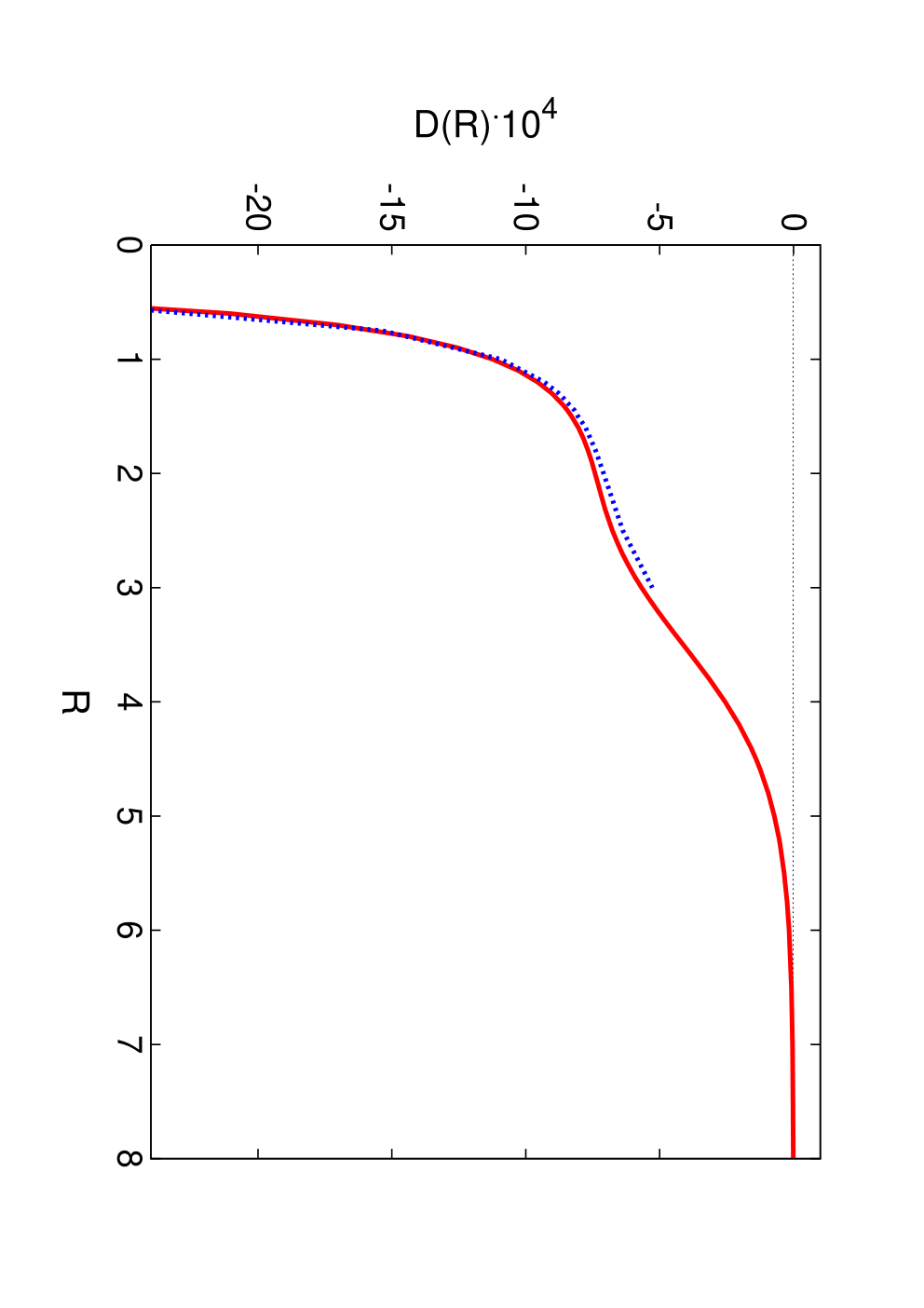
Numerical values of the D⁡(R)D(R) function are presented in Table 1

Table 1: D⁡(R)D(R)—the electric dipole moment (in 10−410^{-4}D) as a function of the internuclear distance RR. All digits are numerically significant.
R/auR/\mathrm{au} D⁡(R)D(R) R/auR/\mathrm{au} D⁡(R)D(R)
0.50.5 −27.6224-27.6224 3.23.2 −5.0893-5.0893
0.60.6 −21.0635-21.0635 3.33.3 −4.7735-4.7735
0.70.7 −17.0294-17.0294 3.43.4 −4.4482-4.4482
0.80.8 −14.3747-14.3747 3.53.5 −4.1182-4.1182
0.90.9 −12.5426-12.5426 3.63.6 −3.7882-3.7882
1.01.0 −11.2339-11.2339 3.83.8 −3.1468-3.1468
1.11.1 −10.2754-10.2754 4.04.0 −2.5552-2.5552
1.21.2 −9.5603-9.5603 4.24.2 −2.0342-2.0342
1.31.3 −9.0193-9.0193 4.44.4 −1.5928-1.5928
1.41.4 −8.6054-8.6054 4.54.5 −1.4022-1.4022
1.451.45 −8.4353-8.4353 4.64.6 −1.2307-1.2307
1.51.5 −8.2853-8.2853 4.84.8 −0.9409-0.9409
1.61.6 −8.0347-8.0347 5.05.0 −0.7137-0.7137
1.71.7 −7.8352-7.8352 5.25.2 −0.5381-0.5381
1.81.8 −7.6721-7.6721 5.255.25 −0.5010-0.5010
1.91.9 −7.5336-7.5336 5.55.5 −0.3495-0.3495
2.02.0 −7.4102-7.4102 5.755.75 −0.2428-0.2428
2.12.1 −7.2933-7.2933 6.06.0 −0.1682-0.1682
2.22.2 −7.1758-7.1758 6.56.5 −0.0804-0.0804
2.32.3 −7.0517-7.0517 7.07.0 −0.0384-0.0384
2.42.4 −6.9156-6.9156 7.57.5 −0.0184-0.0184
2.52.5 −6.7632-6.7632 8.08.0 −0.0089-0.0089
2.62.6 −6.5913-6.5913 8.58.5 −0.0044-0.0044
2.72.7 −6.3972-6.3972 9.09.0 −0.0022-0.0022
2.82.8 −6.1799-6.1799 9.59.5 −0.0012-0.0012
2.92.9 −5.9390-5.9390 10.010.0 −0.0006-0.0006
3.03.0 −5.6755-5.6755 11.011.0 −0.0002-0.0002
3.13.1 −5.3911-5.3911 12.012.0 −0.0001-0.0001

and plotted in Figure 1.

Refer to caption
Figure 1: (Color online) Electric dipole moment function D⁡(R)D(R) (in 10−410^{-4}D). Comparison to previous calculations by Ford and Browne [15] (dotted line). n→\vec{n} is directed from deuteron to proton. Negative D⁡(R)D(R) means that electrons are shifted toward the deuteron.

For comparison with previous calculations, the dipole moment function obtained by Ford and Browne [15] in the range of R∈⟨0.5,3.0⟩R\in\langle 0.5,3.0\rangle au is presented in the same Figure  1. The function D⁡(R)D(R) behaves as R−2R^{-2} at R→0R\to 0, and as R−4R^{-4} at R→∞R\to\infty. The singularity at R=0R=0 comes from the neglecting higher order terms in the unitary transformation and from the adiabatic approximation. At RR of the order me/μn≈0.03\sqrt{m_{\rm e}/\mu_{\rm n}}\approx 0.03 adiabatic approximation fails and our formula for D⁡(R)D(R) is not valid. At this region, however, nuclear wave function is negligible.

For the calculation of the electric dipole moments, the adiabatic potential of the nuclear Schrödinger equation (7) has been composed of the clamped nuclei energy EelE_{\mathrm{el}}, and the adiabatic correction ⟨ϕel|Hn|ϕel⟩\langle\phi_{\rm el}|H_{\mathrm{n}}|\phi_{\rm el}\rangle. For EelE_{\mathrm{el}} we used the energy points computed with nanohartree accuracy by Cencek from 1200-term ECG wave functions [20]. The adiabatic correction in Eq. (8) was evaluated by us using Eq. (40). The adiabatic potential curve was then obtained by means of piecewise polynomial interpolation. The radial Schrödinger equation has been solved numerically using the Le Roy’s code [21]. The obtained nuclear wave functions χ\chi of rovibrational levels were subsequently used in the evaluation of the dipole transition moments of Eq. (18) for the J→J+1J\to J+1 (branch RR) and for the J→J−1J\to J-1 transitions (branch PP).

IV Results and Discussion

Table 2: Experimental and theoretical electric dipole transition moments DfiD_{\rm fi} (in 10−410^{-4}D). Relative uncertainty of our results due to the nonadiabatic corrections to DfiD_{\rm fi} is about 10−310^{-3}.
Reference P⁡(3)P(3) P⁡(2)P(2) P⁡(1)P(1) R⁡(0)R(0) R⁡(1)R(1) R⁡(2)R(2) R⁡(3)R(3)
0-0
experiment [3] 9.36​(30)9.36(30) 8.00​(20)8.00(20) 9.79​(30)9.79(30)
experiment [4] 8.78​(2)8.78(2) 8.47​(2)8.47(2) 10.21​(2)10.21(2)
theory [14] 8.368.36 8.388.38 8.398.39 8.418.41
theory [15] 8.2828.282 8.2978.297 8.3068.306 8.3068.306 8.2978.297 8.2828.282 8.2628.262
theory [16] 8.4408.440 8.4558.455 8.4638.463 8.4638.463 8.4558.455 8.4408.440 8.4208.420
this work 8.5368.536 8.5518.551 8.5608.560 8.5608.560 8.5518.551 8.5368.536 8.5168.516
1-0
experiment [6] 0.330​(40)0.330(40) 0.405​(30)0.405(30) 0.450​(30)0.450(30) 0.515​(20)0.515(20) 0.550​(30)0.550(30) 0.615​(30)0.615(30) 0.655​(40)0.655(40)
experiment [7] 0.340​(22)0.340(22) 0.379​(12)0.379(12) 0.435​(11)0.435(11) 0.504​(12)0.504(12) 0.533​(14)0.533(14) 0.609​(13)0.609(13)
theory [14] 0.5980.598 0.6280.628 0.6560.656 0.6850.685
theory [15] 0.4010.401 0.4450.445 0.4850.485 0.5600.560 0.5940.594 0.6230.623 0.6500.650
theory [16] 0.3740.374 0.4210.421 0.4660.466 0.5520.552 0.5920.592 0.6300.630 0.6650.665
this work 0.37760.3776 0.42480.4248 0.47080.4708 0.55790.5579 0.59830.5983 0.63620.6362 0.67140.6714
2-0
experiment [6] 0.17​(2)0.17(2) 0.19​(2)0.19(2) 0.20​(2)0.20(2)
theory [14] 0.1600.160 0.1660.166 0.1700.170 0.1740.174
theory [15] 0.1560.156 0.1670.167 0.1760.176 0.1920.192 0.1990.199 0.2060.206 0.2100.210
theory [16] 0.1560.156 0.1670.167 0.1790.179 0.2000.200 0.2100.210 0.2190.219 0.2280.228
this work 0.15760.1576 0.16920.1692 0.18050.1805 0.20220.2022 0.21220.2122 0.22160.2216 0.23010.2301
3-0
experiment [6] 0.0795​(35)0.0795(35) 0.0800​(50)0.0800(50)
theory [14] 0.1000.100 0.1020.102 0.1030.103 0.1040.104
theory [15] 0.0680.068 0.0720.072 0.0760.076 0.0820.082 0.0840.084 0.0850.085 0.0870.087
theory [16] 0.06980.0698 0.07420.0742 0.07860.0786 0.08700.0870 0.09090.0909 0.09450.0945 0.09790.0979
this work 0.07050.0705 0.07490.0749 0.07940.0794 0.08780.0878 0.09180.0918 0.09550.0955 0.09890.0989
4-0
experiment [8] 0.0397​(26)0.0397(26) 0.0417​(24)0.0417(24) 0.0425​(21)0.0425(21) 0.0459​(26)0.0459(26) 0.0514​(53)0.0514(53)
theory [14] 0.0560.056 0.0560.056 0.0550.055 0.0530.053
theory [15] 0.0330.033 0.0350.035 0.0380.038 0.0390.039 0.0400.040 0.0420.042 0.0420.042
theory [16] 0.03240.0324 0.03450.0345 0.03650.0365 0.04050.0405 0.04250.0425 0.04420.0442 0.04580.0458
this work 0.03270.0327 0.03480.0348 0.03690.0369 0.04090.0409 0.04280.0428 0.04460.0446 0.04620.0462
5-0
experiment [9] 0.0105​(25)0.0105(25) 0.0124​(21)0.0124(21) 0.0143​(17)0.0143(17) 0.0181​(17)0.0181(17) 0.0200​(21)0.0200(21) 0.0219​(25)0.0219(25) 0.0238​(29)0.0238(29)
experiment [8] 0.0207​(20)0.0207(20) 0.0214​(14)0.0214(14) 0.0231​(21)0.0231(21)
theory [15] 0.0200.020 0.0210.021 0.0210.021 0.0230.023 0.0230.023 0.0240.024 0.0240.024
theory [16] 0.01630.0163 0.01730.0173 0.01840.0184 0.02050.0205 0.02150.0215 0.02250.0225 0.02330.0233
this work 0.01640.0164 0.01750.0175 0.01860.0186 0.02070.0207 0.02170.0217 0.02270.0227 0.02350.0235

Our electric dipole moments for the transitions between the lowest vibrational and rotational levels are listed in Table 2. Except for 0-0 transitions, they are in good agreement with the previous calculation by Thorson et al. For the lowest band all theoretical predictions differ slightly from each other. Our results are numerically accurate to all digits shown, but the last digit is uncertain due to the neglected O⁡(me/μn)≈8×10−4O(m_{\rm e}/\mu_{\rm n})\approx 8\times 10^{-4} higher order nonadiabatic corrections. These corrections have been also neglected in calculations of [15, 16], so in principle these calculations should agree with each other. Considering calculations presented in [14], we note that in the initial expression for D→fi\vec{D}_{\rm fi}, Wolniewicz uses Hn′′H^{\prime\prime}_{\rm n}, Eq. (26), as a perturbation, and assumes the adiabatic approximation for the wave function, but in the denominator he includes Hn′H^{\prime}_{\rm n} from Eq. (15). This expression, in comparison to our, involves some higher order terms, namely X1X_{1} of Eq. (37) from Appendix. However, we show in the Appendix the cancellation of significant contributions involving the second derivative of χ\chi between X1X_{1} and the other higher order contributions X2X_{2} (Eq. (38)) and X3X_{3} (Eq. (39)), which has been neglected in Wolniewicz calculations by assuming the adiabatic wave function. Therefore, we think, slight difference with results of Wolniewicz in [14] may come from less consistent treatment of higher order nonadiabatic effects.

In comparison to experimental values, we observe a moderate agreement for all transitions, but the 0-0 ones. Here, our results, as well as the other theoretical calculations, differ from the experiment by several standard deviations. We note however, that the measurements are most cumbersome for these transitions. As a consequence, experimental values significantly change with the rotational number JJ for v=0v=0, which can not be justified by theoretical analysis. Within the ground vibronic state, the nuclear wave functions corresponding to the lowest rotational levels are localized near the average internuclear distance R0R_{0}, and differ very little from each other. For this reason subsequent transition moments must change slowly with the rotational quantum number JJ, and are approximately equal to D⁡(R0)D(R_{0}), but the experimental results of [3, 4] are not consistent with theoretical predictions.

V Conclusions

We have derived a simple expression for the electric dipole transition rates, in terms of the dipole moment function D⁡(R)D(R), and performed precise calculations of D⁡(R)D(R) in a wide range of RR. The obtained formula, can easily be extended to other diatomic molecules, consisting of two isotopes of the same element. Our results for the dipole moments of HD molecule are numerically accurate to four digits, in moderate agreement with previous calculations in [14, 15, 16] and experimental results of [3, 4, 5, 6, 7, 8, 9] (see Table 2). We estimate, that the relativistic and nonadiabatic corrections are of relative order of 10−410^{-4} and 10−310^{-3}, correspondingly. As no other effect may alter the theoretical predictions, we suppose, that our results are even more accurate than the experimental values obtained so far.

Acknowledgments

We are indebted to L. Wolniewicz for valuable comments.

References

  • [1] G. Herzberg, Nature 166, 563 (1950).
  • [2] M. Trefler and H.P. Gush, Phys. Rev. Lett. 20, 703 (1968).
  • [3] J.B. Nelson and G.C. Tabisz, Phys. Rev. Lett. 48, 1393 (1982).
  • [4] J.B. Nelson and G.C. Tabisz, Phys. Rev. A 28, 2157 (1983).
  • [5] B. Bejar and H.P. Gush, Can. J. Phys. 52, 1669 (1974).
  • [6] A.R.W. McKellar, Can. J. Phys. 51, 389 (1973); Astrophys. J. 185, L53 (1973); Can. J. Phys. 52, 1144 (1974).
  • [7] N. H. Rich, J. W. C. Johns, and A. R. W. McKellar, J. Mol. Spectrosc. 95, 432 (1982).
  • [8] A.R.W. McKellar, W. Goetz, and D.A. Ramsay. Astrophys. J. 207, 663 (1976).
  • [9] F.W. Dalby and J. Vigué, Phys. Rev. Lett. 43, 1310 (1979).
  • [10] G.C. Wick, Atti Reale Accad. Lincei 21, 708 (1935).
  • [11] T.Y. Wu, Can. J. Phys. 30, 291 (1952).
  • [12] S.M. Blinder, J. Chem. Phys. 32, 105 (1960); 32, 582 (1960); 35, 974 (1961).
  • [13] P.R. Bunker, J. Mol. Spectrosc. 46, 119 (1973).
  • [14] L. Wolniewicz, Can. J. Phys. 53, 1207 (1975); 54, 672 (1976).
  • [15] A. L. Ford and J. C. Browne, Phys. Rev. A 16, 1992 (1977).
  • [16] W.R. Thorson, J.H. Choi, and S.K. Knudson, Phys. Rev. A 31, 22 (1985); 31, 34 (1985).
  • [17] H. Abgrall, E. Roueff, and Y. Viala, Astron. Astrophys. Supp. 50, 505 (1982).
  • [18] K. Pachucki and J. Komasa, J. Chem. Phys. 129, 034102 (2008).
  • [19] P.J. Mohr and B.N. Taylor, Rev. Mod. Phys. 77, 1 (2005).
  • [20] W. Cencek, private communication.
  • [21] R. J. Le Roy, University of Waterloo Chemical Physics Research Report CP-663, 2007.

Appendix

For the comparison with previous works [14, 15], which used the term

Hn′′=−12(1MB−1MA)∇→R⋅∑a∇→aH^{\prime\prime}_{\rm n}=-\frac{1}{2}\,\biggl(\frac{1}{M_{B}}-\frac{1}{M_{A}}\biggr)\,\vec{\nabla}_{R}\cdot\sum_{a}\vec{\nabla}_{a} (26)

as a perturbation, we derive the formula for D→fi\vec{D}_{\rm fi}, Eq. (17), using the nonadiabatic perturbation theory. For this, one has to abandon the assumption in Eq. (5) of a separation of the electronic wave function from the nuclear one. Namely, the total wave function

ϕ=ϕa+δ​ϕna=ϕel​χ+δ​ϕna\phi=\phi_{\rm a}+\delta\phi_{\rm na}=\phi_{\rm el}\,\chi+\delta\phi_{\rm na} (27)

will be the sum of the adiabatic solution and a nonadiabatic correction. The nonadiabatic correction δ​ϕna\delta\phi_{\rm na} is decomposed into two parts

δ​ϕna=ϕel​δ​χ+δ′​ϕna,\delta\phi_{\rm na}=\phi_{\rm el}\,\delta\chi+\delta^{\prime}\phi_{\rm na}, (28)

which obey the following orthogonality conditions

⟨δ′​ϕna|ϕel⟩el\displaystyle\langle\delta^{\prime}\phi_{\rm na}|\phi_{\rm el}\rangle_{\rm el} =\displaystyle= 0,\displaystyle 0\,, (29)
⟨δ​χ|χ⟩\displaystyle\langle\delta\chi|\chi\rangle =\displaystyle= 0,\displaystyle 0\,, (30)

with the normalization ⟨ϕ|ϕa⟩=1\langle\phi|\phi_{a}\rangle=1. In the leading order of perturbative treatment, the nonadiabatic corrections to the wave function are the following [18]

|δ′​ϕna(1)⟩\displaystyle|\delta^{\prime}\phi_{\rm na}^{(1)}\rangle =\displaystyle= 1(Eel−Hel)′​Hn​|ϕel​χ⟩,\displaystyle\frac{1}{(E_{\rm el}-H_{\rm el})^{\prime}}\,H_{\rm n}\,|\phi_{\rm el}\,\chi\rangle, (31)
|δ​χ⟩\displaystyle|\delta\chi\rangle =\displaystyle= 1[Ea−Eel−Hn−⟨Hn⟩el]′​⟨ϕel|Hn|δ′​ϕna⟩el,\displaystyle\frac{1}{\bigl[E_{\rm a}-E_{\rm el}-H_{\rm n}-\bigl\langle H_{\rm n}\bigr\rangle_{\rm el}\bigr]^{\prime}}\bigl\langle\phi_{\rm el}\bigl|H_{\rm n}\bigr|\delta^{\prime}\phi_{\rm na}\bigr\rangle_{\rm el},

where the prime in the denominator denotes subtraction of the reference state from the Hamiltonian inversion. For the calculation of D⁡(R)D(R) one needs also the second order correction

|δ′​ϕna(2)⟩\displaystyle|\delta^{\prime}\phi_{\rm na}^{(2)}\rangle =\displaystyle= 1(Eel−Hel)′​Hn​|ϕel​(χ+δ​χ)⟩+1(Eel−Hel)′\displaystyle\frac{1}{(E_{\rm el}-H_{\rm el})^{\prime}}\,H_{\rm n}\,|\phi_{\rm el}\,(\chi+\delta\chi)\rangle+\frac{1}{(E_{\rm el}-H_{\rm el})^{\prime}}
×[Hn+Eel−Ea]​1(Eel−Hel)′​Hn​|ϕel​χ⟩,\displaystyle\times[H_{\rm n}+E_{\rm el}-E_{\rm a}]\,\frac{1}{(E_{\rm el}-H_{\rm el})^{\prime}}\,H_{\rm n}\,|\phi_{\rm el}\,\chi\rangle,

where δ​χ\delta\chi is given by Eq. ().

The derivation of the formula (20) proceeds as follows. One takes Eq. (16) with perturbed wave functions,

D→fi\displaystyle\vec{D}_{\rm fi} =\displaystyle= ⟨ϕel​(χf+δ​χf)+δ′​ϕf,na|r→|ϕel​(χi+δ​χi)+δ′​ϕi,na⟩,\displaystyle\langle\phi_{\rm el}\,(\chi_{\rm f}+\delta\chi_{\rm f})+\delta^{\prime}\phi_{\rm f,na}|\vec{r}|\phi_{\rm el}\,(\chi_{\rm i}+\delta\chi_{\rm i})+\delta^{\prime}\phi_{\rm i,na}\rangle, (34)
=\displaystyle= D→fi(1)+D→fi(2)\displaystyle\vec{D}_{\rm fi}^{(1)}+\vec{D}_{\rm fi}^{(2)}
D→fi(1)\displaystyle\vec{D}_{\rm fi}^{(1)} =\displaystyle= ⟨ϕel​χf|r→​1Eel−Hel​Hn′′|ϕel​χi⟩\displaystyle\langle\phi_{\rm el}\,\chi_{\rm f}|\vec{r}\,\frac{1}{E_{\rm el}-H_{\rm el}}\,H^{\prime\prime}_{\rm n}|\phi_{\rm el}\,\chi_{\rm i}\rangle (35)
+⟨ϕel​χf|Hn′′​1Eel−Hel​r→|ϕel​χi⟩,\displaystyle+\langle\phi_{\rm el}\,\chi_{\rm f}|H^{\prime\prime}_{\rm n}\,\frac{1}{E_{\rm el}-H_{\rm el}}\,\vec{r}|\phi_{\rm el}\,\chi_{\rm i}\rangle\,,

and D→fi(2)\vec{D}_{\rm fi}^{(2)} is given in Eq. (). In the D→fi(1)\vec{D}_{\rm fi}^{(1)} one separates out the electronic matrix elements from the nuclear ones, namely

Dfi(1)​k\displaystyle D^{(1)k}_{\rm fi} =\displaystyle= −12(1MB−1MA)∫d3R{χf⋆χi\displaystyle-\frac{1}{2}\,\biggl(\frac{1}{M_{B}}-\frac{1}{M_{A}}\biggr)\,\int d^{3}R\,\biggl\{\chi^{\star}_{\rm f}\,\chi_{\rm i} (36)
×2​⟨ϕel|rk​1Eel−Hel​∇→R⋅∑a∇→a|ϕel⟩\displaystyle\times 2\,\langle\phi_{\rm el}|r^{k}\,\frac{1}{E_{\rm el}-H_{\rm el}}\,\vec{\nabla}_{R}\cdot\sum_{a}\vec{\nabla}_{a}|\phi_{\rm el}\rangle
+(χf⋆​∇Rjχi+χi​∇Rjχf⋆)\displaystyle+\bigl(\chi^{\star}_{\rm f}\,\nabla_{R}^{j}\chi_{\rm i}+\chi_{\rm i}\,\nabla_{R}^{j}\chi^{\star}_{\rm f}\bigr)
×⟨ϕel|rk1Eel−Hel∑a∇→aj|ϕel⟩},\displaystyle\times\langle\phi_{\rm el}|r^{k}\,\frac{1}{E_{\rm el}-H_{\rm el}}\,\sum_{a}\vec{\nabla}_{a}^{j}|\phi_{\rm el}\rangle\biggr\},

where the superscripts jj and kk are the Cartesian indices. The second term in braces is integrated by parts and Dfi(1)​kD^{(1)k}_{\rm fi} becomes

Dfi(1)​k\displaystyle D^{(1)k}_{\rm fi} =\displaystyle= −12(1MB−1MA)∫d3Rχf⋆χi\displaystyle-\frac{1}{2}\,\biggl(\frac{1}{M_{B}}-\frac{1}{M_{A}}\biggr)\,\int d^{3}R\,\chi^{\star}_{\rm f}\,\chi_{\rm i} (37)
×[⟨ϕ1k|∇Rjϕ2j⟩−⟨∇Rjϕ1k|ϕ2j⟩],\displaystyle\times\bigl[\langle\phi_{1}^{k}|\nabla_{R}^{j}\phi_{2}^{j}\rangle-\langle\nabla_{R}^{j}\phi_{1}^{k}|\phi_{2}^{j}\rangle\bigr],

where

|ϕ1k⟩\displaystyle|\phi_{1}^{k}\rangle =\displaystyle= 1Eel−Hel​rk​|ϕel⟩,\displaystyle\frac{1}{E_{\rm el}-H_{\rm el}}\,r^{k}|\phi_{\rm el}\rangle, (38)
|ϕ2j⟩\displaystyle|\phi_{2}^{j}\rangle =\displaystyle= ∑a∇aj|ϕel⟩\displaystyle\sum_{a}\nabla_{a}^{j}|\phi_{\rm el}\rangle (39)
=\displaystyle= −(Hel−Eel)​me​rj​|ϕel⟩.\displaystyle-(H_{\rm el}-E_{\rm el})\,m_{\rm e}\,r^{j}\,|\phi_{\rm el}\rangle.

One takes ∇→R\vec{\nabla}_{R} of the Schrödinger equation (6) to obtain

∇Rjϕel\displaystyle\nabla^{j}_{R}\phi_{\rm el} =\displaystyle= 1(Eel−Hel)′​∇Rj(V)​ϕel,\displaystyle\frac{1}{(E_{\rm el}-H_{\rm el})^{\prime}}\,\nabla^{j}_{R}(V)\,\phi_{\rm el}, (40)
∇Rjϕ1k\displaystyle\nabla^{j}_{R}\phi^{k}_{1} =\displaystyle= 1Eel−Hel[∇Rj(V−Eel)1Eel−Helrkϕel\displaystyle\frac{1}{E_{\rm el}-H_{\rm el}}\,\biggl[\nabla^{j}_{R}(V-E_{\rm el})\,\frac{1}{E_{\rm el}-H_{\rm el}}\,r^{k}\,\phi_{\rm el} (41)
+rk1(Eel−Hel)′∇Rj(V)ϕel],\displaystyle+r^{k}\,\frac{1}{(E_{\rm el}-H_{\rm el})^{\prime}}\,\nabla^{j}_{R}(V)\,\phi_{\rm el}\biggr],
∇Rjϕ2j\displaystyle\nabla^{j}_{R}\phi^{j}_{2} =\displaystyle= −∇Rj(V−Eel)​me​rj​ϕel\displaystyle-\nabla^{j}_{R}(V-E_{\rm el})\,m_{\rm e}\,r^{j}\,\phi_{\rm el}
+(Eel−Hel)​me​rj​1(Eel−Hel)′​∇Rj(V)​ϕel.\displaystyle+(E_{\rm el}-H_{\rm el})\,m_{\rm e}\,r^{j}\,\frac{1}{(E_{\rm el}-H_{\rm el})^{\prime}}\,\nabla^{j}_{R}(V)\,\phi_{\rm el}.

The gradient of the electronic functions with respect to the internuclear distance in Eq. (37) is replaced by Eqs. (41) and (). Among the four terms, two cancel out and the two other are the same, so the transition dipole moment takes the form

Dfi(1)​k\displaystyle D^{(1)k}_{\rm fi} =\displaystyle= (meMB−meMA)​∫d3​R​χf⋆​χi\displaystyle\biggl(\frac{m_{\rm e}}{M_{B}}-\frac{m_{\rm e}}{M_{A}}\biggr)\,\int d^{3}R\,\chi^{\star}_{\rm f}\,\chi_{\rm i} (43)
×⟨ϕel|rk​1Eel−Hel​r→⋅∇→R​(V−Eel)|ϕel⟩.\displaystyle\times\langle\phi_{\rm el}|r^{k}\,\frac{1}{E_{\rm el}-H_{\rm el}}\,\vec{r}\cdot\vec{\nabla}_{R}(V-E_{\rm el})\,|\phi_{\rm el}\rangle.

One notes that it differs from Eq. (20) only by the presence of ∇→R​Eel\vec{\nabla}_{R}E_{\rm{el}}. We show below, that this term cancels out with Dfi(2)​kD^{(2)k}_{\rm fi} given by

D→fi(2)\displaystyle\vec{D}_{\rm fi}^{(2)} =\displaystyle= ⟨ϕel​χf|​r→​1(Eel−Hel)′​[Hn+Eel−Ei,a]\displaystyle\langle\phi_{\rm el}\,\chi_{\rm f}|\vec{r}\,\frac{1}{(E_{\rm el}-H_{\rm el})^{\prime}}\,[H_{\rm n}+E_{\rm el}-E_{\rm i,a}]
×1(Eel−Hel)′​Hn​|ϕel​χi⟩\displaystyle\times\frac{1}{(E_{\rm el}-H_{\rm el})^{\prime}}\,H_{\rm n}\,|\phi_{\rm el}\,\chi_{\rm i}\rangle
+⟨ϕel​χf|​Hn​1(Eel−Hel)′​r→​1(Eel−Hel)′​Hn\displaystyle+\langle\phi_{\rm el}\,\chi_{\rm f}|\,H_{\rm n}\,\frac{1}{(E_{\rm el}-H_{\rm el})^{\prime}}\,\vec{r}\,\frac{1}{(E_{\rm el}-H_{\rm el})^{\prime}}\,H_{\rm n}
×|ϕel​χi⟩+⟨ϕel​χf|​Hn​1(Eel−Hel)′\displaystyle\times|\phi_{\rm el}\,\chi_{\rm i}\rangle+\langle\phi_{\rm el}\,\chi_{\rm f}|H_{\rm n}\,\frac{1}{(E_{\rm el}-H_{\rm el})^{\prime}}
×[Hn+Eel−Ef,a]​1(Eel−Hel)′​r→​|ϕel​χi⟩.\displaystyle\times[H_{\rm n}+E_{\rm el}-E_{\rm f,a}]\frac{1}{(E_{\rm el}-H_{\rm el})^{\prime}}\,\vec{r}\,|\phi_{\rm el}\,\chi_{\rm i}\rangle.

where we neglected δ​χ\delta\chi. For low lying rovibrational states δ​χ/χ\delta\chi/\chi is small, namely of O⁡(me/μn)O(m_{\rm e}/\mu_{\rm n}) and thus its magnitude is of order 10−310^{-3}, if not less, and thus negligible. HnH_{\rm n} is decomposed into the even Hn′H^{\prime}_{\rm n}, Eq. (15), and the odd Hn′′H^{\prime\prime}_{\rm n} parts Eq. (26). D→fi(2)\vec{D}_{\rm fi}^{(2)} involves the terms with a single power of Hn′H^{\prime}_{\rm n}. The resulting 6 terms in D→fi(2)\vec{D}_{\rm fi}^{(2)} we group into pairs as follows

D→fi(2)\displaystyle\vec{D}_{\rm fi}^{(2)} =\displaystyle= X→1+X→2+X→3,\displaystyle\vec{X}_{1}+\vec{X}_{2}+\vec{X}_{3}, (45)
X→1\displaystyle\vec{X}_{1} =\displaystyle= ⟨ϕel​χf|​r→​1(Eel−Hel)​[Hn′+Eel−Ei,a]\displaystyle\langle\phi_{\rm el}\,\chi_{\rm f}|\vec{r}\,\frac{1}{(E_{\rm el}-H_{\rm el})}\,[H^{\prime}_{\rm n}+E_{\rm el}-E_{\rm i,a}] (46)
×\displaystyle\times 1(Eel−Hel)​Hn′′​|ϕel​χi⟩+⟨ϕel​χf|​Hn′′​1(Eel−Hel)\displaystyle\frac{1}{(E_{\rm el}-H_{\rm el})}\,H^{\prime\prime}_{\rm n}\,|\phi_{\rm el}\,\chi_{\rm i}\rangle+\langle\phi_{\rm el}\,\chi_{\rm f}|H^{\prime\prime}_{\rm n}\,\frac{1}{(E_{\rm el}-H_{\rm el})}
×\displaystyle\times [Hn′+Eel−Ef,a]​1(Eel−Hel)​r→​|ϕel​χi⟩,\displaystyle[H^{\prime}_{\rm n}+E_{\rm el}-E_{\rm f,a}]\frac{1}{(E_{\rm el}-H_{\rm el})}\,\vec{r}\,|\phi_{\rm el}\,\chi_{\rm i}\rangle,
X→2\displaystyle\vec{X}_{2} =\displaystyle= ⟨ϕel​χf|Hn′​1(Eel−Hel)′​r→​1(Eel−Hel)​Hn′′|ϕel​χi⟩\displaystyle\langle\phi_{\rm el}\,\chi_{\rm f}|H^{\prime}_{\rm n}\,\frac{1}{(E_{\rm el}-H_{\rm el})^{\prime}}\,\vec{r}\,\frac{1}{(E_{\rm el}-H_{\rm el})}\,H^{\prime\prime}_{\rm n}\,|\phi_{\rm el}\,\chi_{\rm i}\rangle
+\displaystyle+ ⟨ϕel​χf|Hn′′​1(Eel−Hel)​r→​1(Eel−Hel)′​Hn′|ϕel​χi⟩,\displaystyle\langle\phi_{\rm el}\,\chi_{\rm f}|H^{\prime\prime}_{\rm n}\,\frac{1}{(E_{\rm el}-H_{\rm el})}\,\vec{r}\,\frac{1}{(E_{\rm el}-H_{\rm el})^{\prime}}\,H^{\prime}_{\rm n}\,|\phi_{\rm el}\,\chi_{\rm i}\rangle,
X→3\displaystyle\vec{X}_{3} =\displaystyle= ⟨ϕel​χf|r→​1(Eel−Hel)​Hn′′​1(Eel−Hel)′​Hn′|ϕel​χi⟩\displaystyle\langle\phi_{\rm el}\,\chi_{\rm f}|\vec{r}\,\frac{1}{(E_{\rm el}-H_{\rm el})}\,H^{\prime\prime}_{\rm n}\,\frac{1}{(E_{\rm el}-H_{\rm el})^{\prime}}\,H^{\prime}_{\rm n}\,|\phi_{\rm el}\,\chi_{\rm i}\rangle
+\displaystyle+ ⟨ϕel​χf|Hn′​1(Eel−Hel)′​Hn′′​1(Eel−Hel)​r→|ϕel​χi⟩.\displaystyle\langle\phi_{\rm el}\,\chi_{\rm f}|H^{\prime}_{\rm n}\,\frac{1}{(E_{\rm el}-H_{\rm el})^{\prime}}\,H^{\prime\prime}_{\rm n}\,\frac{1}{(E_{\rm el}-H_{\rm el})}\,\vec{r}\,|\phi_{\rm el}\,\chi_{\rm i}\rangle.

Hn′H^{\prime}_{\rm n} involves two derivatives over RR and Hn′′H^{\prime\prime}_{\rm n} a single derivative. Consider terms with three derivatives of χ\chi. Since χ\chi satisfies Eq. (7), the second derivative of χ\chi coming from Hn′H^{\prime}_{\rm n} cancels with Ea−Eel​(R)E_{\rm a}-E_{\rm el}(R), leaving a small term ⟨Hn′⟩el\langle H^{\prime}_{\rm n}\rangle_{\rm el} and the derivative of EelE_{\rm el}. Thus no term with three derivatives of χ\chi is present. We will show below that no terms involving any derivatives of χ\chi are present. Each X→i\vec{X}_{i} includes two derivatives terms

X1k\displaystyle X_{1}^{k} ≈\displaystyle\approx 12​μn(1MB−1MA)∫d3R[χf∗(∇Rl∇Rjχi)\displaystyle\frac{1}{2\,\mu_{n}}\,\biggl(\frac{1}{M_{B}}-\frac{1}{M_{A}}\biggr)\,\int d^{3}R\,\bigl[\chi^{*}_{\rm f}\,(\nabla_{R}^{l}\,\nabla_{R}^{j}\,\chi_{\rm i})
+χi(∇Rl∇Rjχf∗)]⟨ϕel|rk1Eel−Helrj|∇Rlϕel⟩,\displaystyle+\chi_{\rm i}\,(\nabla_{R}^{l}\,\nabla_{R}^{j}\,\chi^{*}_{\rm f})\bigr]\,\langle\phi_{\rm el}|r^{k}\,\frac{1}{E_{\rm el}-H_{\rm el}}\,r^{j}|\nabla_{R}^{l}\phi_{\rm el}\rangle,
X2k\displaystyle X_{2}^{k} ≈\displaystyle\approx 12​μn(1MB−1MA)∫d3R[(∇Rlχf∗)(∇Rjχi)\displaystyle\frac{1}{2\,\mu_{n}}\,\biggl(\frac{1}{M_{B}}-\frac{1}{M_{A}}\biggr)\,\int d^{3}R\,\bigl[(\nabla_{R}^{l}\chi^{*}_{\rm f})\,(\nabla_{R}^{j}\,\chi_{\rm i})
+(∇Rjχf∗)(∇Rlχi)]⟨ϕel|rjrk1Eel−Hel|∇Rlϕel⟩,\displaystyle+(\nabla_{R}^{j}\chi^{*}_{\rm f})\,(\nabla_{R}^{l}\,\chi_{\rm i})\bigr]\,\langle\phi_{\rm el}|r^{j}r^{k}\,\frac{1}{E_{\rm el}-H_{\rm el}}|\nabla_{R}^{l}\phi_{\rm el}\rangle,
X3k\displaystyle X_{3}^{k} ≈\displaystyle\approx −X1k−X2k,\displaystyle-X_{1}^{k}-X_{2}^{k}\,, (51)

but all of them cancel out in the sum. A single derivative of χ\chi has to be of the form ∇→R​(χf∗​χi)\vec{\nabla}_{R}(\chi^{*}_{\rm f}\,\chi_{\rm i}), what can be integrated by parts and transformed into derivatives of ϕel\phi_{\rm el} and the resolvent. Considering terms without derivatives of χ\chi all of them are of order O⁡[(me/mn)2]O[(m_{\rm e}/m_{\rm n})^{2}] but one, which involves ∇→R​Eel\vec{\nabla}_{R}E_{\rm el} which arised from the commutator [Hn′+Eel​(R)−Ea,∇→R][H^{\prime}_{\rm n}+E_{\rm el}(R)-E_{\rm a},\vec{\nabla}_{R}] in X1X_{1} in Eq. (46). It is of the form

D→fi(2)=(meMB−meMA)​⟨ϕel​χf|r→​1(Eel−Hel)′​r→⋅∇→R​(Eel)|ϕel​χi⟩\vec{D}_{\rm fi}^{(2)}=\biggl(\frac{m_{\rm e}}{M_{B}}-\frac{m_{\rm e}}{M_{A}}\biggr)\,\langle\phi_{\rm el}\chi_{\rm f}|\vec{r}\frac{1}{(E_{\rm el}-H_{\rm el})^{\prime}}\vec{r}\cdot\vec{\nabla}_{R}\,(E_{\rm el})|\phi_{\rm el}\chi_{\rm i}\rangle (52)

which together with D→fi(1)\vec{D}_{\rm fi}^{(1)} gives the leading correction to the transition dipole moment Eq. (17).