Stochastic Resonance in the Fermi-Pasta-Ulam Chain
Abstract
We consider a damped -Fermi-Pasta-Ulam chain, driven at one boundary subjected to stochastic noise. It is shown that, for a fixed driving amplitude and frequency, increasing the noise intensity, the system’s energy resonantly responds to the modulating frequency of the forcing signal. Multiple peaks appear in the signal to noise ratio, signalling the phenomenon of stochastic resonance. The presence of multiple peaks is explained by the existence of many stable and metastable states that are found when solving this boundary value problem for a semi-continuum approximation of the model. Stochastic resonance is shown to be generated by transitions between these states.
pacs
05.40.-a, 73.43.Lp, 05.45.-aSince its theoretical discovery [1, 2] and experimental verification [3, 4] stochastic resonance has become one of the most spread topics in many different branches of physics, biophysics and chemistry (see Ref. [5] for a review). It has a wide variety of applications, e.g. in semiconductors, in neuronal systems, electronic and magnetic systems and, recently, even in quantum physics. All these studies are unified by the common idea to represent a bistable system as particle motion in a double well potential. According to this simplification the system begins to jump from one well to the other, following the periodic forcing, when a resonant noise level is attained. These concepts have wide applications to optical systems. In the ring laser, bistability is due to the left-right propagation symmetry of the system, while in absorptive optical media it is a consequence of the existence of different output powers corresponding to the same input pump intensity [6]. This latter situation has some similarities with the system we discuss in this Letter.
This approach cannot be straightforwardly applied to spatially extended systems, where different stable and metastable excited regimes can coexist, expecially when the forcing is applied locally. As discussed in [7], the presence of metastable states does not hinder stochastic resonance. In this Letter, we show that stochastic resonance can be realized for the well-known Fermi-Pasta-Ulam (FPU) chain [8] of anharmonic oscillators. Up to now stochastic resonance in coupled one dimensional systems has been considered only when each element of the chain displays bistable properties [9, 10]. In our case, bistability characterizes the whole chain, being originated by the coexistence of different stationary regimes corresponding to a single driving amplitude. This coexistence is also at the basis of the nonlinear bistability effect [11, 12, 13] which appears when the chain is harmonically driven at one end with out-band frequency and is due to presence of breather like excitations [14] in the system.
The equations of motion for the -FPU chain (interparticle potential with quadratic and quartic terms) are


| (1) | |||||
where stands for the displacement of the -th unit mass of the chain in dimensionless units (); is the damping parameter (fixed throughout the paper to ) and is a zero average Gaussian white noise applied independently to each oscillator with the following autocorrelation function
| (2) |
We force the system at the left end as follows
| (3) |
while the right boundary condition is free
| (4) |
As commented below, the value of should not be too large, in all simulations presented here .
In Fig. 1 we display several characteristic features of stochastic resonance in the FPU chain. Let us first concentrate the attention on the top-right plot, where we show the signal to noise ratio in decibels. Those who are familiar with stochastic resonance may be surprised to observe multiple peaks in this plot while, usually, a bell shaped curve with a single maximum is found. We will explain below this observation, providing an analytical argument based on the continuum limit of the FPU model. The presence of multiple peaks derives from the existence of multiple stable and metastable states for a given forcing amplitute (the equivalent of having multiple wells in the potential). The forcing signal (3), shown in the central graph in Fig. 1, has a carrier frequency which is chosen slightly above the upper edge of the linear spectrum in order to excite breather type localisations, and is modulated with a much smaller frequency . This latter frequency plays the role of the forcing frequency appearing in standard stochastic resonance. There is a wide range of values of both and for which we can observe stochastic resonance in FPU, given that we respect the important condition . It must be however remarked that the amplitude should be in a range where a stable stationary state of the chain, discussed below, coexists with a metastable one. When this condition is met, we vary the noise strength until we observe the typical oscillations of the energy of the system shown in the lower graph of Fig. 1. The power Fourier spectrum of the energy signal shows a sharp peak at the driving frequency when the noise intensity is at resonance (top-left graph in Fig. 1).
We develop below our analytical approach. Let us begin by solving the boundary value problem for the FPU chain in the absence of damping and noise. It is well known that the FPU chain is characterized by the following linear dispersion relation , hence the spectrum has band edge frequency . In order to derive stationary weakly nonlinear solutions (see e.g. Ref. [15]) of Eq. (1), we seek for solutions of the following standard form [16, 17]:
| (5) |
where denotes the complex conjugated term and varies slowly with respect to both its arguments and . These solutions should be considered as modulations of upper band edge oscillations. The boundary value problem (3) can be rewritten for in the form
| (6) |
where the second condition derives from . Moreover, the condition must be satisfied for the function to be slowly varying with time.
Substituting then (5) into Eqs. (1), and assuming to be a continuous function of its variables, one gets, in the weakly nonlinear limit and neglecting higher order derivatives in and , the following nonlinear Schrödinger equation [16, 17]:
| (7) |
We now assume that the system synchronizes with the boundary (6) and define a new parameter
| (8) |
(where is a real function of ) and, as a result, we get the following relation
| (9) |

and its solution in terms of Jacobi elliptic functions [18, 12], which, after substitution into Eqs. (8) and (5) gives the following approximate solution for the relative displacements of the oscillators
| (10) |
where is the complete elliptic integral of the first kind with a modulus and all the constant are defined via the single free parameter as follows
| (11) |
The free parameter is defined by the condition of adaptation to the boundary (3), leading to the following consistency relation
| (12) |
From this equation one gets all compatible values of for a fixed driving amplitude . It turns out that there are multiple values of that solve Eq. (12), which in turn implies the existence of multiple compatible patterns of the type (10), which have correspondingly different energies. In Fig. 2 we display these energies as a function of the driving amplitude . Three branches of solutions are present. For instance, considering the forcing amplitude , five possible energy values are found: among these two are unstable, two are stable and one is metastable, as described in the caption of Fig. 2. For the type 1 and 2 solutions in Fig. 2, one has an excellent correspondence between the analytical expression (10) and the direct numerical simulations of the FPU chain. For type 3 solutions the approximation is not as good and, besides that, the solution is metastable: in numerical simulations it destabilizes and restabilizes during time evolution. We do not display in Fig. 2 solutions corresponding to higher energies, because the semi-continuouum approximation fails and one should use truncated wave approximations [19].
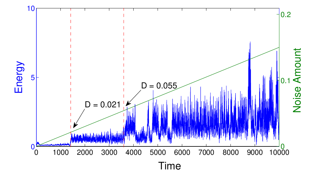
Summarizing, the system is characterized by several threshold amplitudes. When the driving amplitude exceeds the first threshold , the type 1 stable state jumps into the type 2 stable state. By further increasing the driving up to the second threshold , the transition to the type 3 metastable state occurs. In the presence of damping, when reducing the amplitude of the driving, the system does not remain in the higher energy states. Indeed, a lower threshold amplitude appears, , below which the system goes back to the lowest energy stable state. Afterwards, when we will consider stochastic resonance, we will modulate the driving signal in such a way that its amplitude remains above and below (typically ), in order to realize stochastic transitions between all states. Furthermore, we note that for a fixed driving amplitude the stable and metastable states are characterized by sufficiently far separated energies. The presence of these “energy levels” can be monitored by keeping the driving amplitude constant and changing the noise intensity, as shown in Fig. 3. It is clearly seen that for the fixed boundary driving amplitude the transition between type 1 and type 2 stable states occurs at the noise intensity , while at the system goes from a type 2 stable state to a type 3 metastable state. One should also observe that the averaged energies of each state well correspond to the ones derived from the approximate analytical solutions (10).

Now we are ready to discuss the main result of this paper. Simulating the FPU model (1) with the driving signal seed frequency and modulating frequency , such that the driving signal amplitude varies in the range , in the presence of both damping and noise, we monitor the time evolution of the system’s energy for increasing noise intensities , and then analyse the properties of its power spectrum . The signal to noise ratio (SNR) is defined as , where is the frequency at which the power spectrum displays a clear peak (see the top-left plots in Fig. 1) and is the power of the background noise at the same frequency. For low noise intensities there is no transition between the different states and the system’s energy oscillates around . For the noise intensity value (bottom graph in Fig. 1) one observes an oscillation between the state with energy and that with energy . Increasing further noise intensity, the SNR drops and the energy fluctuates around the value (middle plot in Fig. 4 for ). Finally, for the noise intensity , which corresponds to the second peak of the SNR in Fig. 1, we observe noisy transitions between the metastable state of energy and two stable states with energies and (see the bottom graph of Fig. 4). We do not discuss here the smooth third peak observed in Fig. 1, which should be connected to transitions with higher energy states, of which we do not possess a clear analytical characterization.
As remarked above, we have performed all our numerical analysis for short FPU chains (throughout the paper ), but the observation of this phenomenology is not restricted to this case. Indeed, it should be mentioned that, if in the equations for the -FPU chain (1) we would have rescaled the strength of the nonlinear coupling to , the semi-continuum approach developed here would have produced exactly the same solutions (10), provided that the number of particles would have been increased maintaining the ratio constant.
Concluding, we have considered a damped -FPU chain forced at one boundary with a modulated signal under the action of an increasing noise level. For specific values of the noise intensity, the power spectrum of the system’s energy displays sharp peaks at the modulating frequency. Correspondingly, also the signal to noise ratio shows pronounced peaks as a function of noise intensity. This is a clear observation of stochastic resonance in an extended system. In contrast to all previous studies, multiple peaks of the SNR are observed, instead of a single broad bump. In order to explain this feature, we have developed a semi-continuum analytical approach, which allows to point out the presence of multiple stable and metastable solutions for a given forcing amplitude. Stochastic resonance is shown to be generated by transition between these states. These studies could be readily extended to realistic physical systems with local forcing.
Acknowledgements.
R. Kh. acknowledges financial support of the Georgian National Science Foundation (Grant No GNSF/STO7/4-197) and the USA Civilian Research and Development Foundation (award No GEP2-2848-TB-06). This work is part of the PRIN07 project Statistical physics of strongly correlated systems at and out of equilibrium: exact results and quantum field theory methods.
References
- [1] R. Benzi, G. Parisi, A. Sutera, A. Vulpiani, Tellus 34, 10, (1982); R. Benzi, A. Sutera, A. Vulpiani, J. Phys. A, 14, L453, (1981).
- [2] C. Nicolis, Sol. Phys., 74, 473 (1981); C. Nicolis, G. Nicolis, Tellus 33, 225, (1981).
- [3] S. Fauve, F. Heslot, Phys. Lett., 97A, 5, (1983).
- [4] B. McNamara, K. Wiesenfeld, Phys. Rev. A, 39, 4854, (1989).
- [5] L. Gammaitoni, P. Hanggi, P. Jung, F. Marchesoni, Rev. Mod. Phys., 70, 223, (1998).
- [6] E. Arimondo, B.M. Dinelli, Opt. Commun. 44, 277, (1983).
- [7] A. Longtin, J. Stat. Phys. 70, 309, (1993).
- [8] E. Fermi, J. Pasta, S. Ulam, M. Tsingou, in The Many-Body Problems, edited by D.C. Mattis (World Scientific, Singapore, 1993 reprinted); G. Gallavotti (Ed.) The Fermi-Pasta-Ulam Problem: A status report, Springer (2008).
- [9] J. Lindner et al., Phys. Rev. Lett., 75, 3 (1995); M. Inchiosa, A. Bulsara, Phys. Rev. E, 52, 327 (1995); J.F. Lindner, S. Chandramouli, A.R. Bulsara, M. Locher, W.L. Ditto, Phys. Rev. Lett. 81, 5048 (1998).
- [10] M. Locher, G. A. Johnson, E. R. Hunt, Phys. Rev. Lett. 77, 4698 (1996).
- [11] R. Khomeriki, J. Leon, Phys. Rev. E., 71, 056620, (2005).
- [12] R. Khomeriki, J. Leon, Phys. Rev. Lett., 94, 243902, (2005)
- [13] R. Khomeriki, S. Lepri, S. Ruffo, Phys. Rev. E, 70, 066626 (2004).
- [14] T. Dauxois, R. Khomeriki, F. Piazza, S. Ruffo, Chaos 15, 015110 (2005).
- [15] S. Flach and C.R. Willis, Phys. Rep., 295, 181 (1998).
- [16] Yu. A. Kosevich, S. Lepri, Phys. Rev. B, 61, 299, (2000).
- [17] R. Khomeriki, Phys. Rev. E, 65, 026605, (2002).
- [18] P. F. Byrd, M. D. Friedman, Handbook of Elliptic Integrals for Engineers and Physicists, (Springer, Berlin, 1954).
- [19] Yu. A. Kosevich, Phys. Rev. Lett. 71, 2058 (1993) and Phys. Rev. B, 47, 3138, (1993).