Quantum phase transition in the one-dimensional period-two and uniform compass model

Recently, the quantum compass model was introduced to describe some Mott insulators with orbit degeneracy by a pseudospin[1, 2], where the coupling along one of bonds is an Ising type, but different spin components are active along other bond directions. The disorder effect in this model was also examined[3]. The protected qubit is formed if it is separated from the low-energy excitations by a pseudo-spin excited gap. So a high quality factor, scalable and error-free scheme of quantum computation can be designed[4]. The symmetry of pseudo-spin Hamiltonians is usually much lower than SU(2)[5], and the result of numerical calculation has been shown that its eigenstates are at least twofold degenerate or highly degenerate and disordered[6]. The quantum XX-ZZ model, also called one-dimensional (1D) compass model, is constructed by antiferromagnetic order of X and Z pseudo-spin components on odd and even bonds, respectively[7]. In addition, the 1D quantum compass model is exactly the same as the 1D reduced Kitaev model[8]. The analytic eigenspectra in the latter model have been obtained, and it was shown that this model has one gapless phase. But the characters of the quantum phase transition have never been well studied previously. The realistic models of the orbital degeneracy are more complicated.

For the compass model, the pseudo-spins may lead to enhanced quantum fluctuations near the quantum phase transitions (QPTs) and to entangled spin-orbital ground states. The numerical results have indicated that a first-order QPT occurs at $J_{x}=J_{z}$ between two different states with spin ordering along either x or z directions[6]. Recently, the ground-state (GS) fidelity [9, 10, 11, 12, 13, 14, 15] and entanglement [16, 17, 18, 19, 20, 22, 21, 23, 24] emerged from quantum information science have been used in signaling the QPTs. To calculate these quantities accurately, it is necessary to know the exact GS wave function. The derivatives of the GS energy are intrinsically related to the GS fidelity[13], both can be used to identify the QPTs. For the special case of two spin $-1/2$ system, the entanglement is given by the concurrence. Quantum entanglement is one of the most striking consequences of quantum correlation in many-body systems, shows a deep relation with the QPT[16]. Therefore understanding the entanglement is very important in QPTs[17, 18]. In the context of QPTs, the quantum entanglement have been the subject of considerable interests in the Dicke model [19, 20, 21] and the XY model [23, 22].

On the other hand, experimental works on quasicrystals [25] and quasiperiodic superlattices [26] have inspired theoretical interests in 1D quasiperiodic systems. Period-two chain can be regarded as the intermediate one between uniform periodic chain and quasiperiodic chain, which have exhibited some unusual physical properties. In this work, we study the one-dimensional compass model for both uniform and period-two cases by using transfer matrix method[24] and the method of Lieb, Schultz, and Mattis[27]. The exact solutions for two cases are obtained. The GS fidelity and the energy gap between uniform and period-two quantum spin chain are calculated. The behaviors of the pseudo-spin correlations with periodic boundary condition are given.

The paper is organized as follows: In Section II, we give the model and the exact solution with periodic boundary condition. The calculation methods of fidelity and concurrence are introduced in Section III. The correlation functions are analyzed in Section IV. The paper is summarized in Section V, where we give some discussions and conclusions.

The Hamiltonian of one-dimensional compass model is given by

where $J_{i}$ is the nearest-neighbor interaction, $\sigma_{i}^{x(z)}$ are the Pauli matrix on site $i$, $N=2N^{\prime}$ is the number of the sites, and $\beta$ is the coupling parameter which determines the phase transition point. For $J_{2i}=J$ and $J_{2i+1}=\alpha J$ , the model is a period-two case. By using the pseudo-spin (orbital) transformation method which is given by Brzezicki et al[7], we can define the modulated interactions for odd pairs of pseudo-spins $\{2i-1,2i\}$ as $-\tau_{i}^{z}\equiv\sigma_{2i-1}^{z}\sigma_{2i}^{z}$, and the spin-flip operators of $x$ direction are given by $\tau_{i}^{x}\equiv(-1)^{\sum_{k=1}^{i-1}s_{k}}\prod_{j=2i}^{2N^{\prime}}\sigma_{j}^{x}$. The two neighboring odd bonds can be expressed as the even $\{2i,2i+1\}$ bonds by a product $-\tau_{i}^{x}\tau_{i+1}^{x}$. Then the Hamiltonian of one-dimensional compass model can be written as follows

Note that it looks like but is different from the transverse field Ising model.

The vector $\vec{s}$ represents the state $(s_{1},\cdots,s_{N^{\prime}})$. Here $s_{i}=1$ ($s_{i}=0$) labels that the two pseudo-spins of the odd bond $\{2i-1,2i\}$ are parallel (antiparallel). $s=\sum_{i=1}^{N^{\prime}}s_{i}$ is the number of parallel odd pairs of spins. In this paper, we only discuss the ferromagnetic boundary condition of the quantum compass model, i.e. the case of the even $s$. The effective Hamiltonian (2) can be solved by using the Jordan-Wigner transformation for spin operators,

where $c_{i}$ and $c_{i}^{\dagger}$ are the anticommuting fermion operators. After this transformation, The effective Hamiltonian becomes

with

Because we assume that the parity of $s$ is even, it implies that only states with even numbers of Bogoliubov quasiparticles in the spectrum of the Hamiltonian (5). Under the periodic boundary condition $(c_{N^{\prime}+1}=c_{1})$, the number of $c$ fermions must be odd parity, as can easily be obtained from equation (6). Then the general form of the Hamiltonian is simplified to

For the period-two case, we can rewrite (7) as the following form by neglecting the last constant term,

where the nonzero elements of the matrices A and B are given by

Equation (8) can be diagonalized by using the Bogoliubov transformation

where $\psi_{ki}$ is the eigenvector of the matrix $(\textbf{A}+\textbf{B})(\textbf{A}-\textbf{B})$ and $\phi_{ki}$ is that of the matrix $(\textbf{A}-\textbf{B})(\textbf{A}+\textbf{B})$. The eigenvalues of both matrices are corresponding to $\Lambda_{k}^{2}$. We take $k=0,\pm\frac{2\pi}{N^{\prime}},\pm 2\frac{2\pi}{N^{\prime}},\ldots,\pi$. This relation is satisfied with the periodic boundary condition. In general, the two eigenvectors ($\phi_{ki}$ and $\psi_{ki}$) satisfy the following equations

where $\vec{\phi}_{k}$ and $\vec{\psi}_{k}$ are two column vectors. The diagonalized result takes the form

The excitation energies $\Lambda_{k}\geq 0$. At zero temperature, the QPT points are those parameters that satisfy the condition $\Lambda_{k}=0$, and the two coupled coefficients of the Bogoliubov transformation satisfy the following equations:

which can be derived from equation (10). For the period-two case, i.e. $J_{2i}=J$ and $J_{2i+1}=J\alpha$, if we take $J=1$ and assume that $\psi_{k,2n}=Ae^{i2nk}$ and $\psi_{k,2n+1}=Be^{i(2n+1)k}$, the exact results of $\Lambda_{k}$ can be obtained analytically from the coupled equations (12) by using the trace map method. The result is expressed as

The excitation energies have two branches ($\Lambda_{k-}$ and $\Lambda_{k+}$). For a special case $\alpha=1$, i.e., the uniform periodic chain, the excitation energies can be simplified as $2J\sqrt{1+\beta^{2}-2\beta\cos k}$, which is the same as that in Ref. [7]. The QPT point is determined by $\Lambda_{k-}$. At the critical point, the equation can be decoupled for $\Lambda_{k}=0$. One of equation (12) is rewritten as $\phi_{k,i+1}=\frac{1}{\beta}\phi_{k,i}$. Due to the periodic boundary condition, $(\frac{1}{\beta})^{N^{\prime}}=1$ should be satisfied. The only possibility is $\beta=1$, i.e., there is only one QPT point at $\beta=1$ in this case. On the other hand, the GS energy is expressed as $E_{0}=-\frac{1}{2}\sum_{k}\Lambda_{k}$ which includes the spectra of the $\pm$ branches. In thermodynamic limit, the summation can be replaced by an integral

The pseudo-spin excitation gap $\Delta$, which is energy difference between the first excited state and the ground state, is equal to $\Lambda_{0-}$, which disappears at $\beta=1$.

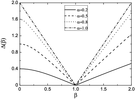
From the Fig.1, we can find that the symmetries of the pseudo-spin gaps are broken more obviously as $\beta$ is away from the QPT point in the period-two model. The symmetries remain for the uniform model. The quantum critical point is fixed at $\beta_{c}=1$ which separates the disorder phase. In the vicinity of the quantum critical point, the linear relation $\Delta=\sqrt{10(\alpha^{2}+1)-2\sqrt{25\alpha^{4}+14\alpha^{2}+25}}|1-\beta|$ is generally satisfied.

The exact GS wave function of the system must be obtained in order to calculate the fidelity and concurrence. Similar to the Bardeen, Cooper, and Schrieffer GS wave function, we can write the present GS wavefunction as[28]:

According to equation (9) and the definition of the fidelity[11]

where $\delta$ is a small quantity ($\delta=10^{-4}$ is taken in our calculation), the fidelity and its susceptibility can be given by

The numerical results for the GS fidelity and its susceptibility are plotted in Fig. 2. An abrupt jump occurs in the vicinity of the QPT point ($\beta_{c}=1$) as a consequence of the dramatic change of the structure of the GS. It agrees exactly with our analytical derivations. One can see level-crossing at $\beta=\beta_{c}$, indicating the first-order QPT in this model.

In recent years, the concept of concurrence is usually adopted as the measure of the entanglement in spin $-\frac{1}{2}$ systems. We will give the nearest-neighbor pseudo-spin two-point correlation functions to calculate the nearest-neighbor concurrence (NNC) of the system. Because of the reflection symmetry, the global phase flip symmetry, and the Hamiltonian being real, the nonzero elements are given by [18, 27]

where $G_{i,j}=-\sum_{k}\psi_{ki}\phi_{kj}$. The definition of concurrence is given by $C(i,j)=max[r_{1}(i,j)-r_{2}(i,j)-r_{3}(i,j)-r_{4}(i,j),0]$, where $r_{\alpha}(i,j)$ are the square roots of the eigenvalues of the product matrix $R=\rho_{ij}\tilde{\rho_{ij}}$ in descending order. The spin flipped matrix $\tilde{\rho_{ij}}$ is defined as $\tilde{\rho_{ij}}=(\sigma^{y}\otimes\sigma^{y})\rho_{ij}^{*}(\sigma^{y}\otimes\sigma^{y})$. The $\rho_{ij}$ is the density matrix for a pair of qubits from a multi-qubit state. In this way, we can calculate the NNC of pseudo-spins. For the period-two chain, the concurrence $C_{2i,2i+1}$ and $C_{2i+1,2i+2}$ are different. So we use the average concurrence $C=\frac{1}{2}(C_{2i,2i+1}+C_{2i+1,2i+2})$.

The numerical results for the concurrence as a function of $\beta$ are given in Fig. 3. It is shown that the maximum value of the concurrence gradually increases with the increase of parameter $\alpha$. If $\alpha$ is small enough, the entanglement of nearest-neighbor pseudo-spins disappears in the larger $\beta$ regime. A cusp of the first derivative of the concurrence occurs at the critical point $\beta=1$, similar to those in Ref. [16].

A gap is found in the curve of NNC versus $\beta$ at the QPT point $\beta_{c}$ in our calculation of the pseudo-spin concurrence. If the pseudo-spin chain goes to infinite, the gap has the critical behavior with $\Delta C\propto N^{-1}$, as shown in the inset of Fig.4. Obviously, it is the finite-size effect. The question then arises: what is the origin of the concurrence gap? The answer is the symmetry of system which has been assumed by the ferromagnetic even-pseudo-spin chains with periodic boundary condition in this paper. The QPT in the 1D compass model is of first-order[4, 7], the scaling behaviors at the critical point should be absent. But the discontinuousness of the concurrence at the QTP may exhibit the finite-size scaling behavior $N\to-1$[29], consistent with the present observation. Due to the concurrence gap, the value of $\partial_{\beta}C$ becomes minimum at the critical point. However, the maximum value of the concurrence occurs below $\beta_{c}$ is not related to the critical point. The present results for the concurrence are similar to those in the periodic quantum Ising chain model[18].

Firstly, we show the numerical results of the ground-state spin correlations on odd $\{2i-1,2i\}$ and even $\{2i,2i+1\}$ bonds as a function of $\beta$ with a periodic boundary condition. The value of $<\sigma_{2i-1}^{z}\sigma_{2i}^{z}>$ gradually increases with $\beta$ while $<\sigma_{2i}^{x}\sigma_{2i+1}^{x}>$ decreases with $\beta$, as shown in Fig. 5. The crossing points of $<\sigma_{2i-1}^{z}\sigma_{2i}^{z}>$ and $<\sigma_{2i}^{x}\sigma_{2i+1}^{x}>$ curves for the same $\alpha$ occur at the quantum critical point. Actually, the compass model is a kind of pseudo-spin Ising chains at $\beta=0$ and $\beta\to\infty$. As a result, the curves of spin correlations versus $\beta$ are asymmetric. So $<\sigma_{2i-1}^{z}\sigma_{2i}^{z}>\to 0$ and $<\sigma_{2i}^{x}\sigma_{2i+1}^{x}>\to-1$ as $\beta\to\infty$.

It is found that the correlation gradually increases with the decreasing $\alpha$. When $\alpha=1$, the numerical result at the critical point is the same as the analytical result by Brzezicki et al. [7].

Finally, we calculate the distance dependence of the pseudo-spin correlator $<\tau_{i}^{x}\tau_{i+r}^{x}>$ under the periodic boundary condition for the period-two and uniform cases. The the two-point correlation function is given by[27]

which has the form of Toeplitz determinant. When $r\to\infty$, the correlators gradually decrease and approach the asymptotic value for large $r$ in an algebraic way[7]. This correlator is positive for all $r$, indicating that there is the long-range ferromagnetic order. It is interesting to find that the oscillation occurs for $\alpha\neq 1$, i.e. for period-two chain, which can be attributed to the different coupling coefficients of odd and even bonds. However, the similar trend appears in both cases, as shown in Fig. 6.

By using the pseudo-spin transformation method and the trace map method, we obtain the exact solution of one-dimensional compass model with periodic boundary condition. The parameter $\alpha$ determines the symmetries of finite pseudo-spin excitation gap $\Delta$, but the phase transition point is still fixed at $\beta=1$. The quantum critical point separates the disorder phase. The pseudo-spin liquid disordered ground state is the universal features in the 1D compass model. The numerical methods to calculate the fidelity and concurrence are also given. We observe a first-order quantum phase transition between two different disordered phase. The concurrence gap $\Delta C$ displays the scaling property $N=-1$. The spin and pseudo-spin correlation functions are calculated. Curves for the two spin correlation function cross exactly at the critical point for any value of $\alpha$. It is observed that the distance dependence of $<\tau_{i}^{x}\tau_{i+r}^{x}>$ correlator displays oscillation in the period-two case, and a divergent correlation length at the critical point is observed in both uniform and period-two chains.

We acknowledge useful discussions with Peiqing Tong and Guang-Ming Zhang. This work was supported by National Natural Science Foundation of China, PCSIRT (Grant No. IRT0754) in University in China, National Basic Research Program of China (Grant No. 2009CB929104), Zhejiang Provincial Natural Science Foundation under Grant No. Z7080203, and Program for Innovative Research Team in Zhejiang Normal University.

^∗ Corresponding author. Email:qhchen@zju.edu.cn

References

- [1] B.Doucot, M. V. Feigel’man, L. B. Ioffe, and A. S. Ioselevich, Phys. Rev. B 71, 024505 (2005).
- [2] A. Mishra, M. Ma, F.-C. Zhang, S. Guertler, L.-H. Tang, S. L. Wan, Phys. Rev. Lett. 93, 207201 (2004).
- [3] T. Tanaka and S. Ishihara, Phys. Rev. Lett. 98, 256402 (2007).
- [4] H. D. Chen, C. Fang, J. P. Hu, and H. Yao, Phys. Rev. B 75, 144401 (2007).
- [5] J. van den Brink, New J. Phys. 6, 201 (2004).
- [6] J. Dorier, F. Becca, and F. Mila, Phys. Rev. B 72, 024448 (2005).
- [7] W. Brzezicki, J. Dziarmaga, A. M.Ole, Phys. Rev. B 75, 134415 (2007).
- [8] X. Y. Feng, G. M. Zhang, and T. Xiang, Phys. Rev. Lett. 98, 087204 (2007).
- [9] H. T. Quan, Z. Song, X. F. Liu, P. Zanardi, and C. P. Sun, Phys. Rev. Lett. 96, 140604 (2006).
- [10] W. L. You, Y. W. Li, and S. J. Gu, Phys. Rev. E 76, 022101 (2007); S. J. Gu, H. M. Kwok, W. Q. Ning, and H. Q. Lin, Phys. Rev. B 77, 245109(2008).
- [11] P. Buonsante and A. Vezzani, Phys. Rev. Lett. 98, 110601 (2007).
- [12] M. Cozzini, R. Ionicioiu, and P. Zanardi, Phys. Rev. B 76, 104420 (2007).
- [13] S. Chen, L. Wang, Y. J. Hao, and Y. P. Wang, Phys. Rev. A 77, 032111 (2008).
- [14] H. Q. Zhou, R. Orus, G. Vidal, Phys. Rev. Lett. 100, 080601 (2008); H. Q. Zhou, J. P. Barjaktarevic, arXiv:cond-mat/0701608.
- [15] T. Liu, Y. Y. Zhang, Q. H. Chen, and K. L. Wang, arXiv: 0812.0321.
- [16] A. Osterloh, L. Amico, G. Falci, and R. Fazio, Nature (London) 416, 608(2002); S. J. Gu, H. Q. Lin, and Y. Q. Li, Phys. Rev. A 68, 042330(2003).
- [17] P. Q. Tong and X. X. Liu, Phys. Rev. Lett. 97, 017201 (2006).
- [18] L. F. Zhang and P. Q. Tong, J. Phys. A 38, 7377 (2005).
- [19] N. Lambert, C. Emary, and T. Brandes, Phys. Rev. Lett. 92, 073602(2004).
- [20] G. Liberti, F. Plastina, and F. Piperno, Phys. Rev. A 74, 022324 (2006). J. Vidal and S. Dusuel, Europhys. Lett. 74, 817(2006)).
- [21] Q. H. Chen, Y. Y. Zhang, T. Liu, and K. L. Wang, Phys. Rev. A 78, 051801(R) (2008).
- [22] J. Reslen, L. Quiroga, and N. F. Johnson, Europhys. Lett. 69, 8(2005).
- [23] T. J. Osborne and M. A. Nielsen, Phys. Rev. A. 66, 032110(2002); G. Vidal, J. L. Latorre, E. Rico, and A. Kitaev, Phys. Rev. Lett. 90, 227902 (2003).
- [24] P. Q. Tong and M. Zhong, Phys. Rev. B 65, 064421 (2002).
- [25] D. Shechtman, I. Blech, D. Gratias, and J.W. Cahn, Phys. Rev. Lett. 53, 1951 (1984)
- [26] R. Merlin, K. Bajema, R. Clarks, F.Y. Juang, and P.K. Bhattacharya, Phys. Rev. Lett. 55, 1768 (1985)
- [27] E. Lieb, T. Schultz and D. Mattis, Ann. Phys., NY 16, 407 (1961).
- [28] M. C. Chung and I. Peschel, Phys. Rev. B 64, 064412 (2001).
- [29] T. M. Liaw, M. C. Huang, S. C. Lin and Y. P. Luo, cond-mat/0408393v1