Modeling the Decay of Entanglement for Electron Spin Qubits in Quantum Dots
Abstract
We investigate the time evolution of entanglement under various models of decoherence: A general heuristic model based on local relaxation and dephasing times, and two microscopic models describing decoherence of electron spin qubits in quantum dots due to the hyperfine interaction with the nuclei. For each of the decoherence models, we investigate and compare how long the entanglement can be detected. We also introduce filtered witness operators, which extend the available detection time, and investigate this detection time for various multipartite entangled states. By comparing the time required for detection with the time required for generation and manipulation of entanglement, we estimate for a range of different entangled states how many qubits can be entangled in a one-dimensional array of electron spin qubits.
pacs
03.65.Ud, 03.67.Mn, 73.21.LaI Introduction
Entanglement refers to non-classical correlations between two [1, 2, 3, 4] or more [6, 5] quantum particles, and the creation of multiparticle entangled states constitutes a key step towards quantum computation [7]. In this work, we investigate the evolution of entangled states under different models of decoherence: a heuristic model with a broad range of applications, and two microscopic models specific for electron spin qubits in quantum dots [8]. We show how entanglement can be detected, and how fast this needs to be done before the states become disentangled by decoherence. We also estimate for four different classes of multipartite entanglement which class survives the longest, and how many entangled qubits can be generated and detected with actual experimental means and currently known decoherence times.
We consider decoherence of a local nature, i.e. the qubits decohere in an uncorrelated way, as is the case in solid-state nanosystems such as electron spin qubits in quantum dots [8], various superconducting qubits [9] and other solid-state implementations [10]: In these systems, the decoherence can be characterized phenomenologically [11] by a relaxation time and a dephasing time . The microscopic origin of the decoherence is still a matter of intensive research: In this paper we discuss some microscopic models for electron spin qubits in quantum dots and compare them with this heuristic model.
Our proposed means to analyze entanglement are so-called witness
operators [12, 13, 14, 15, 16]: locally decomposable observables with a positive
expectation value for all separable states, and a negative expectation value for at least one
entangled state. The advantage of entanglement witnesses over other methods such as e.g. full
state tomography is that they require less measurements, and thus less experimental effort to
detect and prove the existence of entanglement for a given (mixed) state. Witnesses have
intensively been used in experiments with photons [17, 18] and trapped
ions [19], but so far only few theoretical proposals exist for using witness operators in
solid-state nanosystems [20].
This paper is organized as follows: in Sec. II we briefly summarize the mechanisms influencing the time scales and for electron spin qubits. We describe two theoretical models of dephasing for these qubits and compare them to the heuristic master equation model. We also show how we calculate the decoherence of a multipartite state of separated qubits using the Lindblad formalism. Next (Sec. III) we demonstrate our main ideas and methods using the simplest case of two qubits, compare the different models of decoherence and introduce our filtered witness operator. In Sec. IV we consider both GHZ- and W-states for three qubits. In Sec. V we do the same for four qubits and consider in addition the cluster and Dicke entanglement classes. We also discuss the dependence of the decay of entanglement on the initial state. Finally, in Sec. VI, we discuss the case of qubits: We show that the entanglement of a specific GHZ-state can theoretically be detected for any finite time, and discuss the feasibility of generating and detecting many-qubit entangled states of electron spin qubits based on decoherence and operation time scales that have been measured in recent experiments on single and double quantum dots.
II Decoherence model
Decoherence is caused by uncontrolled interactions between the qubit and the environment [21]. This effect is usually characterized by two time scales, the phase randomization time (“dephasing time”) and the time in which the excited state relaxes to the ground state by energy exchange with the environment (“relaxation time”) [11]. For electron spin qubits (as for most solid-state qubits) the dephasing time is much shorter than the relaxation time, , and is therefore the dominant time scale for the loss of quantum correlations. In this section, we consider both a simple exponential model of decoherence based on these two time scales, as well as use two microscopic descriptions of dephasing for electron spin qubits in quantum dots to derive more sophisticated time evolutions of decoherence.
We start by briefly discussing decoherence mechanisms for electron spin qubits.
The original idea by Loss and DiVincenzo [22] proposed to confine single electrons in a
quantum dot (an island of charge in a two-dimensional electron gas) and apply a magnetic field to
split the degeneracy of the spin-up and spin-down states, thus creating a two-level system serving
as carrier for quantum information: an electron spin qubit. Two electron spin qubits interact via a
Heisenberg coupling, and this interaction can be controlled by tuning the potential barrier between
two neighboring dots [23]. Single qubit operations rely on electron spin resonance and
can be performed by applying local electric or magnetic fields [24, 25].
Decoherence – interaction with the environment – is mainly
mediated by two processes, spin-orbit interaction and hyperfine interaction [8].
Spin-orbit interaction does not have a direct effect on the electron spin, since the electrons do
not move, but it leads to a mixing of spin and orbital degrees of freedom [26]. In GaAs
quantum dots, spin-orbit interaction is estimated to be small – both experimentally [27] and
theoretically [28] – compared to the hyperfine interaction with the nuclei, so that the
latter is the dominant source of dephasing.
If the atoms of the semiconductor material have a non-zero nuclear magnetic moment (as for example in GaAs; in other materials, such as purified SiC, this effect is not present), the electron spin interacts with the nuclear spins via the hyperfine interaction [29]: the Hamiltonian for such a system can be written as [31, 32]
| (1) |
Here, () is the electron (nuclear)
Zeeman splitting [calculated using the Bohr (nuclear) magneton (, where
) and the effective -factor of the electron (nuclei), (),
which in GaAs takes the value ]. Next, is
the sum over the -component of all nuclear spins , and denotes the quantum field of the nuclei acting on the electron
spin, where are the number of nuclei whose wave function overlaps with the electron’s wave
function ( for typical dots), denotes the coupling strength between the
-th nucleus and the electron. Since the electron’s wave function is zero outside the dot, there
is no overlap with the nuclei outside the quantum dot – thus each electron in the array couples to
a different bath of nuclei, and the decoherence is thus local, as stated above. Since hyperfine
interaction is the dominant source of noise, we can disregard other types of noise which might
induce some correlations between different qubits, as for example phonons.
For an intuitive semiclassical description of decoherence due to hyperfine interaction the quantum
field of the nuclear spins can be treated as an additional (classical) magnetic field – the
Overhauser field – by replacing . The maximum value this
field can reach in GaAs is about [30] T for fully polarized nuclei. In low
external magnetic fields, the Overhauser field undergoes Gaussian fluctuations around a
root-mean-square value [31, 32, 33] of . The electron thus feels
a total magnetic field which consists of the sum of the controlled external field and
the random Overhauser field . The field’s longitudinal component
(parallel to ) changes the precession frequency of the electron spin by . The transverse part changes the precession frequency even
only in quadratic order, . This random nuclear
magnetic field changes in time: two nuclei with different coupling strength can exchange
their spin, thus leading to a change in the Overhauser field ; these fluctuations appear on
a time scale of s (for a weak external field) [36], but could probably be
extended up to well more than several seconds to minutes (for the longitudinal nuclear field
in a strong external field ) [37].
The bulk dephasing time (at which the fluctuating nuclear magnetic field removes the
phase information) can be measured by rotating the spin in the -plane, let it evolve freely, and
then rotate it back along the -axis for measurement (so-called spin echo measurements). Each
data point then has to be averaged over many measurements, during which the nuclear field evolves.
This leads to an average dephasing time , which has been measured to be about
ns [38].
The dephasing time of a single electron, on the other hand, is very hard to measure, because
it is not possible to measure the initial orientation and strength of the nuclear field with
sufficient precision. Estimates in various regimes predict s: a good way to
estimate is by using a Hahn echo technique, where the free evolution of the spin due to the
initial magnetic field is undone by reversing the spin, but not the dephasing due to the change of
this nuclear field [41]. Assuming Gaussian fluctuations of the nuclear field on a time
scale of s and (a conservatively estimated) ns, a time s can be
extracted [8], which has been confirmed by measurements [23] providing a lower
bound on of s.
For a microscopic, quantum-mechanical treatment of , we rewrite in (1) in a parallel and transversal part [31, 32, 39, 40]
| (2) |
describes a flip-flop interaction between the electron and a nucleus, thus the operators are the raising and lowering operators for the spin () and a nucleus (). This perturbation is small as soon as there is some external magnetic field and the energy mismatch between the electron and the nuclear spin states suppresses it, as discussed above: expressed in numbers, this requires [39], or equivalently (using and low polarisation) , which is fulfilled in typical experiments (with an external field above T; in Refs. [35, 46], for example, fields of up to T are used). A first approximation is to completely neglect this term and only consider the change of precession frequency due to the nuclear field . Using the central limit theorem for a large number of nuclear spins results in a Gaussian distribution for . The transverse correlator, defined as the self correlation function of the transverse spin component, (here, is the initial density matrix of the combined system of electron and nuclei), is given by [39, 40]
| (3) |
As opposed to exponential decay of phase coherence with time scale , (3) represents superexponential decay with a characteristic time : for a GaAs dot with almost no polarization, , one can estimate , which is much faster than the experimentally observed -time. The second, imaginary part represents the coherent rotation induced by the total magnetic field. The value for depends on the initial state of the nuclei: for a pure state with each nucleus having probability for being in the excited state, it can directly be calculated as , where is the hyperfine coupling field.
A more sophisticated approach is to include the perturbation term in (2), and rewrite the von Neumann equation in the form of a Nakajima-Zwanzig generalized master equation (GME) [39]:
| (4) |
Here is the projector on the electron-subspace, the Liouville-operator ( for any operator ) and the self-energy superoperator. Using regular perturbation theory in the parameter (i.e. for a high magnetic field ), some (unphysical) secular terms arise; these terms do not occur by directly expanding in the GME. The latter results in a self correlation function for the transversal spin of the form [39] (in the frame oscillating with a frequency proportional to the Zeeman splitting)
| (5) |
where is the Markovian solution, and is the remainder term, i.e. the difference between the exponential and the non-markovian solution in Born approximation. This can be written as , and solved by iterating to leading order in the parameter (corresponding to a high external field, since ). The solution depends strongly on the wave function of the electron: we assume the electron to have a Gaussian wave function in two dimensions, resulting in
| (6) |
Here we have defined a characteristic time (s for GaAs quantum dots). In a realistic setting, this correction term is very small, since is very small: in GaAs typically . Nonetheless, we will calculate this correction for completeness.
Relaxation of an electron spin qubit is caused by the same two effects as dephasing: spin-orbit and hyperfine interaction. The required energy for the spin-orbit interaction to flip the spin of the electron is provided by the phonons in the lattice of the semiconductors forming the 2DEG, and can be calculated as a function of the external magnetic field [26]. The hyperfine contribution to relaxation manifests itself as flips of the electron spin through exchanging its spin state with a nuclear spin. For increasing external field, the energy mismatch between the nuclear spin states and the electron spin state grows, and more and more energy has to be absorbed by phonons – thus the relaxation can be suppressed by applying a higher external field. The relaxation time has been measured in experiments to range from ms (at ) to s () [34, 35].
In a phenomenological model of decoherence, the time scales and are incorporated into a master equation model for the density matrix with on the diagonal (describing the effect of relaxation) and on the off-diagonal (describing dephasing):
| (7) |
Qualitatively, the off-diagonal phase components decrease exponentially with a rate , and the ground state becomes populated at the expense of the excited state , where the normalization condition () has to be fulfilled at any time . (7) is a general phenomenological model to describe decoherence, and can thus be adjusted to describe decoherence for a wide range of systems, but it does not include microscopic information about the quantum processes causing the decoherence.
We now discuss how to extend these decoherence models [Eqs. (3), (5) and (7)] to more than one qubit. For the exponential decay, this is quite straightforward: we rewrite (7) in the Lindblad formalism [42] using the Lindblad operator :
| (8) | |||||
Here, and are products of the Pauli matrices. Comparing the density matrices resulting from Eqs. (7) and (8), we can identify and . The time evolution of a single qubit is then found by solving . To extend (8) to multipartite states, we write the Lindblad operator for the -th qubit as , where is the -th operator of a total of . The time evolution of the total -partite state is then given by solving as before with . By using this definition we implicitly assumed that the decoherence of each qubit is governed by the same and .
For the two other models, given in (3) and (5), we construct the density matrix of the entangled states in a similar manner. Since the decoherence of the various qubits is assumed to be independent, we can just multiply the corresponding single matrix entries. For statistically distributed quantities (as for example ), we have to consider the addition rules for distributions with the corresponding variances, and furthermore we have to take into account which contributions have to be conjugated (e.g. the precession terms due to the magnetic field).
III Two qubits
Let us first explain our methods and definitions for the simple case of two qubits. A separable state is defined as a state which can be written as a convex combination of product states [1, 2, 4]
| (9) |
where and are states in different subsystems and and the probabilities have to fulfill the normalization condition . If a state is not of this form, it is called entangled.
We use witness operators [12, 6, 13, 14, 15, 16] to investigate the entanglement of various states. An observable is called an entanglement witness if it fulfills the following two requirements:
- 1.
For any separable state , the expectation value of is larger than zero:
separable. - 2.
There must be at least one entangled state for which has a negative expectation value:
.
Therefore, a measured negative expectation value of the witness guarantees that the state is entangled. For the experimental implementation, entanglement witnesses can be decomposed into local measurements (see also below), and they usually require much fewer measurements than procedures such as full state tomography. Thus they are experimentally easier to implement. Finally, it should be noted that witnesses can be used to quantify entanglement, by giving lower bounds on entanglement measures [43].
The witnesses we use in this paper are derived from the so-called projector-like witness [17]:
| (10) |
with the constant standing for the maximum overlap between the state and any separable state. Physically, this witness encodes the fact that if a state has a fidelity larger than , then must be entangled.
We first investigate the time evolution of the Bell state [1, 3] . The choice of this Bell-state, the singlet state, is motivated by the fact that it is the ground state of the quantum system consisting of two electron spins in a double quantum dot [8], thus it is the simplest entangled state that can be created in quantum dots.
The density matrix of a singlet state under exponential decay can be found from Eqs. (7) and (8):
| (11) |
with the factors for relaxation and for dephasing. With that, the fidelity [7] is given by
| (12) |
and the expectation value of the projective witness for is then calculated using (10),
| (13) |
where is the witness for the singlet state, . Figure 1 shows the decay of entanglement for this exponential model of decay of the coherence.

For the other two models of decoherence [Eqs. (3) and (5)], we first have to construct the corresponding density matrix: for the relaxation, we keep the exponential terms , but for the dephasing we use the correlators presented in the previous section. The first model is based on the superexponential dephasing from (3) for each qubit, whose density matrix we label with . We have to calculate the entries and , therefore the conjugation reverses the phase in (3), so the off-diagonal dephasing terms (the star ∗ stands for complex conjugate) are given in terms of the correlators of the -th dot () by:
| (14) | |||||
where the second line is for identical statistics of the dots (thus with identical characteristic times ). Including the boundary condition we obtain the density matrix:
| (15) |
with as before and from (14). The witness operator for detecting (15) is thus the same as in (13) with the replacement . The evolution of the corresponding witness is shown in figure 2 a).
The third model uses the non-markovian Born approximation for the decay, Eqs. (5) and (6). The single electron decay is given by , where the first exponential term stems from the Markovian solution, and the remainder term is given in (6). In order to set up the density matrix in the non-markovian approximation, we replace in (11) by , in the same way as in the super-exponential case.


b) Decay of the entanglement witnesses for the non-markovian approximation, including the correction term to the Markovian solution, for characteristic time s, but an enhanced smallness parameter in order to underline the effect of the correction term.
In the next part we introduce a systematic method to enlarge the time interval during which entanglement can be detected by the witness operators. This method is based on applying local (so-called filtering) operators to the witness operator and analyzing the measurement results in a different way without requiring more measurements. Analyzing the witness (13), we see immediately that it becomes positive (and hence does not detect the entanglement anymore) when after some finite time becomes smaller than , though it can be shown (by virtue of the PPT-criterion [44], for example) that the state is entangled for any , i.e. for any .
Therefore, our goal is to construct a witness operator which is able to detect the entanglement in the state at any time. This can be achieved by a filter operator ,
| (16) |
where the are arbitrary invertible matrices acting on individual qubits. Since is local, application of such a filter operator on a state does not change its entanglement properties, i.e. is entangled, iff is entangled.
Equivalently, one can apply filter operators to witness operators , and the resulting filtered witness operator is then given by
| (17) |
As normalization, we choose , to make the witnesses’ mean values comparable.
Our goal is now to design a filter such that it increases the negativity of the witness, i.e. it should increase the weight of the terms and in (13), so that the filtered witness can be used to detect entanglement during longer times. This can be achieved by the following filter:
| (18) |
with a positive real number. The normalized filtered witness for the singlet state then takes the form
and the expectation value is given by
| (24) |
Clearly, is negative if is chosen large enough and time dependent and (thus ), and the negativity of the witness can be optimized by a suitable choice of for a given time . The remaining entanglement [which is not detected by , (13)] in the decohering state can then be detected by measuring this filtered witness operator. The effectiveness of the filter operator crucially depends on the choice of the singlet state as the initial state: it can easily be shown that for the other Bell states = , the filtered witness does not lead to any improvement over the regular witness operator. The decay of entanglement in our model thus strongly depends on the initial state, even within the same basis.
For the experimental implementation, the witness can be decomposed into single-qubit measurements [15]:
| (25) | ||||
This decomposition requires three measurement settings (namely with ) instead of the nine settings full state tomography would require [14, 45]. Similar decompositions exist for all other witnesses occurring in this paper [17, 47].
In Figs. 1 and 2, the evolution of the expectation values for both the regular witnesses (solid line) and the filtered witnesses (dashed line) are plotted. In the experimentally relevant limit (), the advantage of the filter operator in an experiment does not manifest itself as strongly as would be the case for ; however, the principle advantage that the entanglement can be detected for any finite time is demonstrated in the insets by a zoom into the region where the unfiltered witness becomes positive. The filtered witness remains negative, albeit with a small, exponentially decaying absolute value, for any finite time: this proves that the contains at least a very small amount of entanglement at any time under our decoherence models; however, it will not lead to a significant advantage in an experiment, since the noise due to imperfect state preparation and measurement fidelities will render it virtually impossible to measure the expectation value with such a high precision.
From this curve, one can conclude that it becomes difficult to detect entanglement after more than a few s under realistic conditions assuming any of the decay models we have considered (for the superexponential decay even after a few ns, but for all models the exact time also depends on the size of the error bars in a given experiment). Consequently, any generation scheme for the Bell states which requires a generation time longer than this time will probably not work in practice.
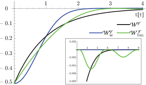
For short times, both the superexponential and the non-markovian approximation are decaying less strongly than the exponential model, but after some time, the witness assuming exponential decay has a greater negativity. The inset compares the longer-time behavior of the three models: the non-markovian approximation features a periodic recurrence of negative values (due to precession around the nuclear magnetic field), and the slowest long-time decay (disregarding the coherent precession).
Let us conclude this section by a comparison of the three models: The evolution of the expectation
values of the filtered witnesses is plotted in figure 3 (all in units of the respective
critical time for the comparison). In the non-markovian approximation, we have chosen the smallness parameter
such that the effect of the correction can be shown. This comparison reveals
benefits and drawbacks of each decay model: first, the filtered entanglement operators are all
negative for any finite time . The entanglement in the superexponential model decays
faster than in the other two, and in the non-markovian approximation, we see the effect of the power-law tail
[the second term in (6)] as a periodic rebouncing due to the precession around the
-component of the nuclear magnetic field, . As a result, the expectation value of this
witness operator is more negative than for the purely exponential decay. In the main plot showing
the short time evolution scaled by the critical time for each model, the differences between the
models are not as pronounced, and they behave roughly the same.
Let us consider a realistic experiment at this point: In an experiment, it is likely that errors
will arise due to imperfect read-out of the electron spin states [35, 46], which will
manifest themselves as error bars on the curves for the time evolution. This error will make it
unlikely to detect the entanglement at longer times in a realistic experiment. Regarding
figure 3 with these errors in mind, the evolution within the three models is
roughly equivalent. Another source of possible experimental inaccuracies is the preparation of the
initial state – in general it will not be the exact aimed-for state, but a mixture of states. This
mixture will influence the use of the witness and the filter operator, which as well strongly
depends on the nature of the mixture; though the precise influence is hard to predict, the filter
will always improve the witness operator to some degree. However, the creation of pure singlet
states in double quantum dots has already been experimentally achieved in a controllable manner and
with high probability of success [23]. Therefore we expect that our noiseless results can
nevertheless be used to give qualitative predictions of the decay of entanglement.
So far, we have considered two entangled qubits and found that their entanglement remains
detectable for about the same time for three decoherence models. When considering generalization to
many qubits, we note that the exponential model features a big advantage compared to the other two,
since for this model there is a general method for calculating the time evolution of the density
matrix for an arbitrary number of qubits (see also Sec. VI), whereas for the two other
models we have to construct the density matrix for each new state by hand. Therefore, in the
following sections, we will use the exponential model for the generalization to multiple qubits.
IV Three Qubits
For three or more particles, the situation is more complicated, since different classes of multiparticle entanglement exist [50, 48, 49].
Let us first discuss the notion of partial separability. A state can be partially separable, meaning that some of the qubit states are separable, but not all. An example for three particles is the state
| (26) |
where is a (possibly entangled) state of two qubits (defined on subsystems and ), and a state of the third qubit (defined on subsystem ). The state is separable with respect to a certain bipartite split, so it is called biseparable. A mixed state is biseparable, if it can be written as mixture of biseparable pure states.
If a state is not biseparable, it is genuinely multipartite entangled. There exist different classes of multipartite entangled states [48] and the number of entanglement classes increases with the number of qubits [51]. An entanglement class can be defined by the following question: given a single copy of two pure states and , is it possible, at least in principle, to transform into (and vice versa) using local transformations only? Even if the probability of success is small? For three qubits, for example, two entanglement classes exist, the GHZ and the W-class. Every genuine multipartite entangled three-qubit state can be transformed into one of the two states [48]
| (27) | |||||
| (28) |
but, remarkably, these two states cannot (not even stochastically) be transformed into each other, and are therefore representatives of different entanglement classes.
Let us now investigate the lifetime of these two states using our exponential decoherence model, described below (8). After calculating the time evolution of the two states, we obtain for the corresponding fidelities:
| (29) | |||||
| (30) |
From these fidelities, the expectation values of the witnesses can directly be determined as for the GHZ state, and for the W state.

Our next step is to apply the filter operators to the witnesses. This yields the following values for the expectation value of the filtered witness operators:
| (31) | |||||
| (32) |
These witness operators can be measured by four (for the GHZ state) or five (for the W state) measurement settings [47], compared to the 27 measurement settings required for full state tomography. In principle, the witness for the W state can be improved by taking the projector onto the subspace with at most two excitations [16], ( instead of ). However, in the present case this does not give any improvement, since the state is not populated. The time evolution of the witness expectation values (31) and (32) are plotted in figure 4 (for s-1 and s-1).
V Four Qubits
The more qubits are added, the more distinct classes of entangled states arise. For four qubits, we investigate the following four classes:
| (33) | ||||
| (34) | ||||
| (35) | ||||
| (36) |
All of these states have been realized in various experiments for different physical systems [52], but so far not in solid-state nanosystems. Also, some of their decoherence properties have been investigated from different theoretical perspectives [54, 53]. The states and are the four-qubit versions of the states we have investigated for three qubits in the previous section. is a representative of the so-called cluster class [55], important in the context of one-way quantum computing [56]. The Dicke state [57] is an extension of the W-state and consists of all possible permutations of states containing 2 excitations. The fidelity of these states evolves as:
| (37) | |||||
| (38) | |||||
| (39) | |||||
| (40) |
The corresponding projective witnesses can be found, as before, using , with for the cluster and GHZ-states, for the W-state, and for the Dicke state [58].
Again, filter operations can be applied: the resulting formulas are lengthy and therefore not given here. The improvement over the regular witness again shows (as for the general case of qubits) that the GHZ-state contains in theory entanglement for any finite time – but so little, that this result is of a theoretical nature and not experimentally relevant. For the other classes of states, the filter can lead to a slightly higher negativity, but not to an extension of the time where the expectation value will become positive. So what is left is to compare the differences in the evolution of the expectation values of these witness operators for the four classes, and to see which one is the most stable, i.e. detectable for the longest time. This is done in figure 5.

At this point the same question can be asked as for the two-qubit state that we investigated in Sec. III: how does the available detection time depend on the exact state chosen as representative of a class? Or, equivalently, the fidelity of which state decoheres most slowly? In fact, writing the states above in a different basis leads to different decay rates.
This is illustrated in figure 6, where the evolution of the witness expectation value of four different cluster states is plotted: from (34), is the original cluster state from Ref. [59] containing 16 terms, and the two additional representations
| (41) | |||||
| (42) | |||||
with 4 and 8 terms, respectively (the first one is a representation with the minimal number of terms, which will be used again in the next section, the second one a rotated version of the original cluster state). As can be seen in figure 6, the detection time decreases as the number of terms increases, though the effect is not very large for four and more terms. The representations with the minimal number of terms thus decohere more slowly. This is not surprising, since one can prove for a similar decoherence model that states with the minimal number of terms are most robust [53]. For representations with the same number of terms, the number of excitations in each term can influence the detectability: which one of the two is easier to detect then depends on the ratio of and .

VI N qubits
Let us now consider the general situation of qubits. We concentrate on three types of entangled states for which there exist proposals how to generate them using available single- and two-qubit operations in quantum dots [60]: GHZ-, W-, and cluster states. Our goal is to calculate the time evolution of the normal (unfiltered) witness for arbitrary and compare this with the time necessary to generate and measure the state. The representatives of the first two classes can be written down straightforwardly (for even ):
| (43) | ||||
| (44) |
Calculating the expectation value of the witness operators leads to (for even ):
| (45) | ||||
| (46) |
The general form of the cluster state – the one we consider here containing the minimal number of terms, namely – is more complicated; it can be written as [61]
| (47) |
where this formula should be understood as an iteration, with the operator acting on the Bell state of the next two qubits. For four qubits, this results exactly in the representation from (41), the evolution of which is plotted in figure 6. To calculate the time evolution of the fidelity, we represent the cluster state (47) as [56]
| (48) |
with a product of Pauli matrices. We incorporate the effects of dephasing (disregarding the relaxation of the qubits, i.e. setting , which leads to an error of less than ‰ for four qubits) in every term in the sum of the expanded (48). The resulting fidelity of the cluster state can then easily be calculated numerically up to qubits.

Figure 7 shows the time at which the expectation value of the (unfiltered) projective witness for each of the three states [Eqs. (45), (46) and (48)] becomes positive as a function of the qubit number , as well as a rough estimate of the time necessary to generate and measure these states. For electron spin qubits in quantum dots the generation times are taken from Ref. [60]: for both the cluster and the W-states the time required to produce these states is independent of the number of qubits, whereas the production time of states of the GHZ-class scales linearly with the number of qubits. The measurement times are composed as follows: measurement distinguishes between spin-up and spin-down (defined along the z-axis [35]) and measuring the components and then requires a rotation of the spins by , which takes about ns [24]. The sum of the generation and the measurement time is given by the lines in the plot.
We see in figure 7 that (as in Figs. 4 and 5) the entanglement of the GHZ-state can be detected for the longest times, but it is more time-consuming to generate than the other two entangled states. Based on the estimates in figure 7, generation and detection of GHZ states should be possible for up to 14 qubits (with the standard projective witness and assuming current operation and decoherence times for electron spin qubits). The cluster state is the state which can be detected for the largest number of qubits, although for up to 12 qubits the “time reserve” (i.e. the difference between the time needed for generation and measurement and the time when the expectation value of the witness operator becomes positive) for the GHZ state is somewhat larger than for the cluster state. The W-state is the least suitable, the largest state would contain about qubits.
Our results for the cluster state show that one-way quantum computing [55] is not really feasible in quantum dots with current dephasing times: we expect that up to maximally qubits could be entangled under the presented preparation scheme, which is far too few for exploiting the advantages of a quantum computer.
Based on our assumptions, thus, the simplest state to generate and prove it’s entanglement would be the GHZ-state for up to twelve qubits, and the cluster state for more than twelve and up to twenty qubits, though the remaining entanglement becomes very small. The same holds for the filtered witness for the GHZ state for an arbitrary number of qubits.
VII Conclusion
In conclusion, we have investigated entanglement and its detectability in a linear array of electron spin qubits which locally undergo decoherence. We have considered three different phenomenological models for the dephasing of the qubits based on exponential and superexponential decay. Using witness operators as detectors of entanglement and introducing a specific class of filtered witness operators, we estimated the maximum available detection time for entanglement of two electrons using each of the models and found that the time during which entanglement is detectable is independent of the model chosen. We then expanded the exponential model to the case of multipartite entanglement: For three and four qubits, we compared the decay of entanglement for different classes of entangled states with each other, namely the GHZ-, W-, cluster and Dicke classes. We also gave limits on the maximum number of entangled qubits that can be created and measured based on currently known decoherence times for electron spin qubits. The most suitable entangled state turns out to be the GHZ-state for up to a few qubits. Our results can help to make a choice as to which state to prepare in experiments. Since local decoherence is characteristic for many types of solid-state qubits, our model and the filtered operator technique are applicable to a variety of these qubits.
This work has been supported by The Netherlands Organisation for Scientific Research (NWO), the FWF (START prize) and the EU (SCALA, OLAQUI, QICS).
References
- [1] A. Einstein, B. Podolski, and N. Rosen, Phys. Rev. 47, 777 (1935).
- [2] E. Schrödinger, Naturwissenschaften 23, 807 (1935).
- [3] J. S. Bell, Physics 1, 195 (1964).
- [4] R. F. Werner, Phys. Rev. A 40, 4277 (1989).
- [5] R. Horodecki, P. Horodecki, M. Horodecki, and K. Horodecki, arXiv:quant-ph/0702225.
- [6] M. Horodecki, P. Horodecki, and R. Horodecki, Phys. Lett. A 223, 1 (1996).
- [7] M. A. Nielsen and I. L. Chuang, Quantum Computation and Quantum Information, (Cambridge University Press, Cambridge, UK, 2000).
- [8] R. Hanson, L. P. Kouwenhoven, J. R. Petta, S. Tarucha, and L. M. K. Vandersypen, Rev. Mod. Phys. 79, 1217 (2007).
- [9] G. Wendin and V. S. Shumeiko, in the Handbook of Theoretical and Computational Nanotechnology, 1, 129; see also arXiv:cond-mat/0508729.
- [10] For a recent overview of more solid-state qubit systems such as e.g. nitrogen-vacancy centers in diamond, see R. Hanson and D. D. Awschalom, Nature 453, 1043 (2008) and references therein.
- [11] See e.g. H.-A. Engel and D. Loss, Phys. Rev. B 65, 195321 (2002).
- [12] B. M. Terhal, Phys. Lett. A 271, 319 (2000).
- [13] M. Lewenstein, B. Kraus, J. I. Cirac, and P. Horodecki, Phys. Rev. A 62, 052310 (2000); B. M. Terhal, Phys. Lett. A 271, 319 (2000).
- [14] O. Gühne, P. Hyllus, D. Bruß, A. Ekert, M. Lewenstein, C. Macchiavello, and A. Sanpera, Phys. Rev. A 66, 062305 (2002).
- [15] O. Gühne, P. Hyllus, D. Bruss, A. Ekert, M. Lewenstein, C. Macchiavello, and A. Sanpera, J. Mod. Opt. 50, 1079 (2003).
- [16] O. Gühne and G. Tóth, Physics Reports 474, 1 (2009).
- [17] M. Bourennane, M. Eibl, C. Kurtsiefer, S. Gaertner, H. Weinfurter, O. Gühne, P. Hyllus, D. Bruß, M. Lewenstein, and A. Sanpera, Phys. Rev. Lett. 92, 087902 (2004).
- [18] C.-Y. Lu, X.-Q. Zhou, O. Gühne, W.-B. Gao, J. Zhang, Z.-S. Yuan, A. Goebel, T. Yang, and J.-W. Pan, Nature Physics 3, 91 (2007).
- [19] D. Leibfried et al., Nature 438, 639 (2005); H. Häffner et al., Nature 438, 643 (2005).
- [20] M. Blaauboer and D. P. DiVincenzo , Phys. Rev. Lett. 95, 160402 (2005); L. Faoro and F. Taddei, Phys. Rev. B 75, 165327 (2007).
- [21] M. Schlosshauer, Rev. Mod. Phys. 76, 1267 (2005).
- [22] D. Loss and D. P. DiVincenzo, Phys. Rev. A 57, 120 (1998).
- [23] J.R. Petta et al., Science 309, 2180 (2005).
- [24] F. H. L. Koppens, C. Buizert, K. J. Tielrooij, I. T. Vink, K. C. Nowack, T. Meunier, L. P. Kouwenhoven, and L. M. K. Vandersypen, Nature 442, 766 (2006).
- [25] K.C. Nowack et al., Science 318, 1430 (2007).
- [26] A. V. Khaetskii and Yu. V. Nazarov, Phys. Rev. B 64, 125316 (2001).
- [27] D. M. Zumbühl, J. B. Miller, C. M. Marcus, K. Campman and A. C. Gossard, Phys. Rev. Lett. 89, 276803 (2002), J. B. Miller, D. M. Zumbühl, C. M. Marcus, Y. B. Lyanda-Geller, G. Goldhaber-Gordon, K. Campman and A. C. Gossard, Phys. Rev. Lett. 90, 076807 (2003).
- [28] V. N. Golovach, A. Khaetskii, and D. Loss, Phys. Rev. Lett. 93, 016601 (2004).
- [29] A. Abragam, The Principles of Nuclear Magnetism, (Oxford University Press, 1961).
- [30] D. Paget, G. Lampel, B. Sapoval, and V. I. Safarov, Phys. Rev. B 15, 5780 (1977).
- [31] A. V. Khaetskii, D. Loss, and L. Glazman, Phys. Rev. Lett. 88, 186802 (2002).
- [32] I. A. Merkulov, A. L. Efros, and M. Rosen, Phys. Rev. B 65, 205309 (2002);
- [33] P.-F. Braun et al., Phys. Rev. Lett. 94, 116601 (2005); A. C. Johnson, J. R. Petta, J. M. Taylor, A. Yacoby, M. D. Lukin, C. M. Marcus, M. P. Hanson, and A. C. Gossard, Nature 435, 925 (2005); F. H. L. Koppens, J. A. Folk, J. M. Elzerman, R. Hanson, L. H. Willems van Beveren, I. T. Vink, H. P. Tranitz, W. Wegscheider, L. P. Kouwenhoven, L. M. K. Vandersypen, Science 309, 1346 (2005); J.M. Taylor et al, Phys. Rev. B 76, 035315 (2007).
- [34] R. Hanson, B. Witkamp, L. M. K. Vandersypen, L. H. Willems van Beveren, J. M. Elzerman, and L. P. Kouwenhoven, Phys. Rev. Lett. 91, 196802 (2003).
- [35] J. M. Elzerman, R. Hanson, L. H. Willems van Beveren, B. Witkamp, L. M. K. Vandersypen, and L. P. Kouwenhoven, Nature 430, 431 (2004).
- [36] R. G. Shulman, B. J. Wyluda, and H. J. Hrostowski, Phys. Rev. 109, 808 (1958).
- [37] This is not confirmed experimentally, but the very slow decay of nuclear spin polarization of up to several minutes is an indication for slow change of ; see e.g. A. K. Hüttel, J. Weber, A. W. Holleitner, D. Weinmann, K. Eberl, and R. H. Blick, Phys. Rev. B 69, 073302 (2004).
- [38] J. M. Kikkawa and D. D. Awschalom, Phys. Rev. Lett. 80, 4313 (1998).
- [39] W.A. Coish and D. Loss, Phys. Rev. B 70, 195340 (2004).
- [40] L. Chirolli and G. Burkard, Advances in Physics 57, 225 (2008), see also arXiv:0809.4716 .
- [41] B. Herzog and E. L. Hahn, Phys. Rev. 103, 148 (1956).
- [42] G. Lindblad, Commun. Math. Phys. 48, 119 (1976).
- [43] F. G. S. L. Brandão, Phys. Rev. A 72, 022310 (2005); D. Cavalcanti and M. O. Terra Cunha, Appl. Phys. Lett. 89, 084102 (2006); O. Gühne, M. Reimpell, and R. F. Werner, Phys. Rev. Lett. 98, 110502 (2007); J. Eisert, F. Brandão, and K. Audenaert, New J. Phys. 9, 46 (2007).
- [44] A. Peres, Phys. Rev. Lett. 77, 1413 (1996); M. Horodecki, P. Horodecki, and R. Horodecki, Physics Letters A 223, 1 (1996).
- [45] G. Tóth and O. Gühne, Phys. Rev. Lett. 94, 060501 (2005).
- [46] R. Hanson, L. H. Willems van Beveren, I. T. Vink, J. M. Elzerman, W. J. M. Naber, F. H. L. Koppens, L. P. Kouwenhoven, and L. M. K. Vandersypen, Phys. Rev. Lett. 94, 196802 (2005).
- [47] O. Gühne and P. Hyllus, Int. J. Theor. Phys. 42, 1001 (2003).
- [48] W. Dür, G. Vidal, and J. I. Cirac, Phys. Rev. A 62, 062314 (2000).
- [49] A. Acín, D. Bruß, M. Lewenstein, and A. Sanpera, Phys. Rev. Lett. 87, 040401 (2001).
- [50] Daniel M. Greenberger, Michael A. Horne, Anton Zeilinger: Bell’s theorem, Quantum Theory, and Conceptions of the Universe, pp. 73-76, (Kluwer Academics, Dordrecht, The Netherlands, 1989), see also arXiv:0712.0921; D. M. Greenberger, M. A. Horne, A. Shimony, and A. Zeilinger, Amer. J. Phys. 58, 1131-43 (1990).
- [51] F. Verstraete, J. Dehaene, B. De Moor, and H. Verschelde, Phys. Rev. A 65, 052112 (2002); L. Lamata, J. León, D. Salgado, and E. Solano, Phys. Rev. A 75, 022318 (2007).
- [52] See e.g. Refs. [17, 18] and [19] for realizations of GHZ, W, and cluster states of up to 8 qubits using photons and ions, respectively, and N. Kiesel, C. Schmid, G. Tóth, E. Solano, and H. Weinfurter, Phys. Rev. Lett. 98, 063604 (2007) for a four-qubit Dicke photon state.
- [53] O. Gühne, F. Bodoky, and M. Blaauboer, Phys. Rev. A 78, 060301(R) (2008).
- [54] C. Simon and J. Kempe, Phys. Rev. A 65, 052327 (2002); W. Dür and H.J. Briegel, Phys. Rev. Lett. 92, 180403 (2004); L. Aolita, R. Chaves, D. Cavalcanti, A. Acín, and L. Davidovich, Phys. Rev. Lett. 100, 080501 (2008); A. Borras, A. P. Majtey, A. R. Plastino, M. Casas, and A. Plastino, Phys. Rev. A 79, 022108 (2009).
- [55] R. Raussendorf and H.-J. Briegel, Phys. Rev. Lett. 86, 5188 (2001), R. Raussendorf, D. E. Browne and H.-J. Briegel, Phys. Rev. A 68, 022312 (2003).
- [56] M. Hein, W. Dür, J. Eisert, R. Raussendorf, M. Van den Nest, and H.-J. Briegel: in Proceedings of the International School of Physics Enrico Fermi on Quantum Computers, Algorithms and Chaos, (Varenna, Italy, 2005); see also arXiv:quant-ph/0602096.
- [57] R. H. Dicke, Phys. Rev. 93, 99 (1954).
- [58] G. Tóth, J. Opt. Soc. Am. B 24, 275 (2007).
- [59] See (2) in H.-J. Briegel and R. Raussendorf, Phys. Rev. Lett. 86, 910 (2001).
- [60] F. Bodoky and M. Blaauboer, Phys. Rev. A 76, 052309 (2007).
- [61] In general, a cluster state is defined as an eigenstate of certain local observables [55, 56]; here we choose them as ; ; ; ; . This is locally equivalent to the definition as in [55, 56]; however, the state given in (47) contains the minimal number of terms; see Ref. [53].