The Approximate Capacity of the Many-to-One and One-to-Many Gaussian Interference Channels

We first introduce the multi-user Gaussian interference channel. For notational simplicity in the sequel, we assume there are $K+1$ users, labeled $0,1,\dots,K$. The channel outputs are related to the inputs by

where for $0\leq i\leq K$, $x_{i}\in\mathbb{C}$ is subject to a unit average power constraint $\frac{1}{N}E||x_{i}^{N}||^{2}\leq P_{i}$ and the noise processes $z_{i}\sim\mathcal{CN}(0,N_{0})$ are i.i.d. over time. The channel gain between input $i$ and output $j$ is denoted by $h_{ji}\in\mathbb{C}$. The signal-to-noise and interference-to-noise ratios are defined as $\mathtt{SNR}_{i}=|h_{ii}|^{2}P_{i}/N_{0}$ for $0\leq i\leq N$, and $\mathtt{INR}_{ij}=|h_{ji}|^{2}P_{i}/N_{0}$ for $0\leq i,j\leq N$, $i\neq j$. Each receiver attempts to decode the message from its corresponding receiver. The remaining (standard) definitions can be found in [2], and generalize naturally to an arbitrary number users.

In this paper we consider two special cases of the Gaussian IC. In the first half we study the Gaussian many-to-one IC, where all gains are zero except $h_{ii}$, $0\leq i\leq K$, and $h_{i0}$, $1\leq i\leq K$. The channel is depicted in Figure 1. In the second half of the paper we treat the Gaussian one-to-many IC, which is obtained from the many-to-one IC by reversing the roles of transmitters and receivers. The one-to-many IC has all gains equal to zero except for $h_{ii}$, $0\leq i\leq K$, and $h_{0i}$, $1\leq i\leq K$.

In the two-user Gaussian IC a simple Han-Kobayashi scheme with Gaussian codebooks was shown to be nearly optimal [2]. A natural question: is the same type of scheme, a (generalized) Han and Kobayashi scheme with Gaussian codebooks, nearly optimal with more than 2 users? We answer this question by way of an example 3-user Gaussian many-to-one channel. This example goes to the heart of the problem and captures the salient features of the many-to-one channel. In particular, the approach used for the two-user interference channel is demonstrated to be inadequate for three or more users, while a simple strategy that aligns interference on the signal scale is shown to be asymptotically optimal.

The example channel is depicted in Figure 2. The power constraints are $P_{0}=P_{1}=P_{2}=1$ and the gains are $h_{00}=h_{01}=h_{02}=\beta$ and $h_{11}=h_{22}=\sqrt{\beta}$.

We first describe the Han-Kobayashi scheme with Gaussian codebooks for the three-to-one channel. In the many-to-one channel each user’s signal causes interference only at receiver 0, so the signals from users 1 and 2 are each split into common and private parts as in the two-user scheme (see [2], [11], for details on the two-user scheme). Each user $i=1,2$ employs a superposition of Gaussian codebooks

with power $P_{U_{i}}+P_{W_{i}}=1$ and rates $R_{U_{i}},R_{W_{i}}$. The “private” signal $U_{i}$ is treated as noise by receiver 0, while the “common” signal $W_{i}$ is decoded by receiver 0. User 0 selects a single random Gaussian codebook with power $P_{0}$ and rate $R_{0}$.

There are two equivalent ways of interpreting the effect of the interference to receiver 0 from users 1 and 2: the first asks how “noisy” is the interference, while the second asks how much of the information content within the interference is available to receiver 0. Both viewpoints are related by the entropy $h(\beta x_{1}+\beta x_{2}+z_{0})$. For the first, we may expand the mutual information relevant to user 0 as $I(x_{0};y_{0})=h(y_{0})-h(\beta x_{1}+\beta x_{2}+z_{0})$. If the second entropy term is large, i.e. the interference is “noisy”, then the rate of user 0 must be small.

Consider now the second viewpoint. Note that the interference to noise ratios $\mathtt{INR}_{1}=\mathtt{INR}_{2}=\beta$ are much larger than the signal-to-noise ratios $\mathtt{SNR}_{1}=\mathtt{SNR}_{2}=\sqrt{\beta}$. Let us momentarily recall a similar situation in the context of the two-user channel: the so-called strong interference regime occurs when the cross-gains are stronger than the direct gains. Hence, after decoding the intended signal, each receiver can decode the interfering signal as well, and thus each signal consists entirely of common information. This means the interference is quite damaging, since it contains the full information content of the intended signal.

Returning to our example channel, let us examine the output at receiver 0, ignoring the intended signal from transmitter 0. The information on $x_{1}$ and $x_{2}$ at receiver 0 is then $I(y_{0};x_{1},x_{2}|x_{0})=h(\beta x_{1}+\beta x_{2}+z_{0})-h(z_{0})$. For our example channel it turns out that when $x_{1}$ and $x_{2}$ are Gaussian distributed, the entropy $h(\beta x_{1}+\beta x_{2}+z_{0})$ is large enough to allow user 0 to decode both of the signals $x_{1}$ and $x_{2}$. Thus, the signals from users 1 and 2 are entirely common information. When all of the signals are common information, it is easy to bound the sum-rate $r_{\text{sum}}^{HK}=r_{0}+r_{1}+r_{2}$, since the rates must lie within the MAC capacity region formed by receiver 0 and the three transmitters. This reasoning yields the following claim.

We now propose a different scheme that achieves a rate point within a constant of the optimal sum-rate of approximately $3\log\beta$ for any $\beta=2^{2n}$, where $n$ is a positive integer. The restriction of $\beta$ to even powers of two allows to simplify the analysis of the scheme; the scheme itself, as well as the general scheme presented in Section 5, works for arbitrary real-valued channel gains. Consider first only the real-valued channel (assume that $z_{i}\sim\mathcal{N}(0,1)$ and inputs are real-valued). Each user generates a random codebook from a discrete distribution

where the bits $x_{i}(k)\sim\text{Bernoulli}\left(\frac{1}{2}\right)$ are i.i.d. over time. In order to show an achievable rate we calculate the single time-step mutual information between input and output for each user,

Let $\tilde{y}_{i}$ denote the noiseless output

It is shown in Appendix A.1 of [13] that when using inputs such that the outputs $\tilde{y}_{i}$ are integer-valued, the additive Gaussian noise $z_{i}$ causes a loss in mutual information of at most 1.5 bits, i.e.

Intuitively, this is because $\tilde{y}_{i}$ can be recovered from $y_{i}$ by knowing the value of $[z_{i}]$, where $[\,\cdot\,]$ is the nearest integer function; the estimate $H([z_{i}])\leq 1.5$ allows to show the inequality (4).

Note the following key observation: it is possible to perfectly recover the signal $x_{0}$ from $\tilde{y}_{0}$. This follows from writing

and the fact that $\sqrt{\beta}x_{0}<\sqrt{\beta}$ . Hence

and for $i=0,1,2$,

For the complex-valued channel the same strategy works independently in the complex and real dimension, giving an achievable rate of

The sum-rate achieved,

is therefore arbitrarily larger than the approximately $2\log\beta$ achieved by the strategy employing Gaussian codebooks. The achievable region for large $\beta$, normalized by $\log\beta$, is depicted in Figure 3.

Before proceeding we reflect on why random Gaussian codebooks are suboptimal for the many-to-one channel. Note that the aggregate interference at receiver 0 has support equal to the sumset of the supports of codebooks 1 and 2. As illustrated in Figure 5, the sumset of two random (continuously distributed) codebooks fills the space, leaving no room for user 0 to communicate. If each of codebooks 1 and 2 have $m$ points, the sumset can have up to $m^{2}$ points. In contrast, as illustrated in Figure 5, the sum of two codebooks that are subsets of a lattice looks essentially like one of the original codebooks (and in particular has cardinality $Cm$, where $C$ is a constant independent of $m$). Thus, the cost to user 0 is the same as though due to only one interferer, i.e. the interference is aligned on the signal scale. This theme will reappear throughout the paper.

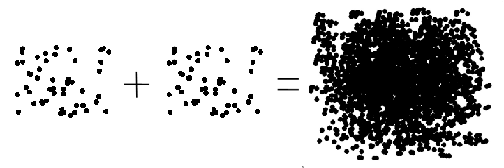
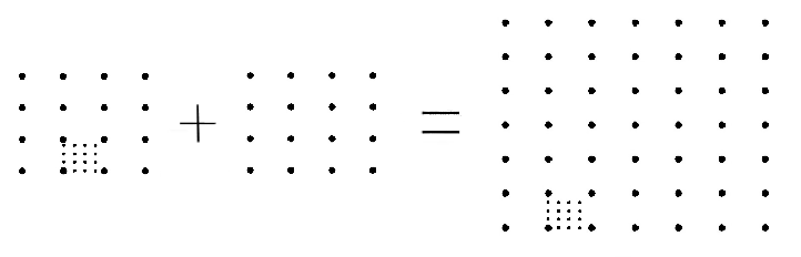
In order to generalize the intuition gained from this example and provide the framework for finding the capacity of the many-to-one channel to within a constant gap we make use of a deterministic channel model, described in the next section.

We proceed with the deterministic interference channel model. Note that the model is completely determined by the model for the MAC. There are $K+1$ transmitter-receiver pairs (links), and as in the Gaussian case, each transmitter wants to communicate only with its corresponding receiver. The signal from transmitter $j$, as observed at receiver $i$, is scaled by a nonnegative integer gain $n_{ij}$. The channel may be written as

where, as before, addition is performed on each bit (modulo two) and $\lfloor\,\cdot\,\rfloor$ is the integer-part function.

Alternatively, at each time $t$, we may view the input and output, respectively, at link $i$ to be $x_{i}(t),y_{i}(t)\in\mathbb{F}_{2}^{q}$, where $q=\max_{ij}n_{ij}$. The channel output at receiver $i$, $0\leq i\leq K$, is given by

where summation and multiplication are in $\mathbb{F}_{2}$ and $\mathbf{S}$ is a $q\times q$ shift matrix (8). The standard definitions of achievable rates and the associated notions are omitted.

The deterministic interference channel is relatively simple, yet retains two essential features of the Gaussian interference channel: the loss of information due to noise, and the superposition of transmitted signals at each receiver. The modeling of noise can be understood through the point-to-point channel above. The superposition of transmitted signals at each receiver is captured by taking the modulo 2 sum of the incoming signals at each level.

The relevance of the deterministic model is greatest in the high-$\mathtt{SNR}$ regime, where communication is interference—rather than noise—limited; however, we shall see that even for finite signal-to-noise ratios the deterministic channel model provides significant insight towards the more complicated Gaussian model.

As in the approach for the Gaussian interference channel, we consider only special cases of the deterministic interference channel: the many-to-one and one-to-many ICs. In the many-to-one IC interference occurs only at receiver 0 (see Figure 8 for an example), and in the one-to-many IC interference is caused by only one user.

The achievable strategy consists of allocating each level separately, by choosing either user 0 to transmit on a given level, or all users interfering with user 0 to transmit on the level. This scheme aligns the interference as observed by receiver 0, so that several users transmitting on a level inflict the same cost to user 0 as one user transmitting on the same level. Because the scheme considers each level separately, the structure of the achievable region is remarkably simple. The region is next described in more detail.

First, note that by transmitting on levels that appear above the signal of user 0 or below the noise level as observed by receiver 0, each user can transmit at rate

where $f_{\text{free}}(i)=(n_{0i}-n_{ii})^{+}+(n_{0i}-n_{00})^{+}$, without causing any interference to user 0. We have that users $\{1,\dots,K\}$ can use rates in the region

without causing any interference to user 0.

For a subset of users $U_{k}\subseteq\{1,\dots,K\}$, let ${\mathcal{C}}_{k}$ denote the capacity region of a deterministic many-to-one IC with only one level, and users $U_{k}$ interfering at receiver 0. Users not in $U_{k}$, i.e. $\{1,\dots,K\}\setminus U_{k}$, are not present. It is easy to see that ${\mathcal{C}}_{k}$ is given by the intersection of the individual rate constraints

and the pair-wise rate constraints

The capacity ${\mathcal{C}}_{k}$ is achieved by time-sharing between two rate points: 1) User 0 transmits a uniformly random bit, while all other users are silent, or 2) User 0 is silent while each user in $U_{k}$ transmits a uniformly random bit. This is done for each level $1\leq k\leq{n_{00}}$.

Let $\underline{{\mathcal{C}}}$ be the set of rate points achieved by our scheme. Since the achievable scheme treats each level separately, the achievable region is the sum of the regions for each level and the set of points achievable without causing any interference:

We now turn to the outer bound, first rewriting the constraints on each level. Consider some level $k$, $1\leq k\leq{n_{00}}$. For any set of users ${\mathcal{S}}\subseteq\{1,\dots,K\}$, we can form a sum-rate constraint on the users ${\mathcal{S}}\cup\{0\}$ by adding a single pairwise constraint on $r_{0}+r_{i}$ for some $i\in{\mathcal{S}}$ together with individual rate constraints on users ${\mathcal{S}}\setminus\{i\}$ (11):

where

The following lemma gives an outer bound $\overline{{\mathcal{C}}}$ to the capacity region. Thus the capacity region, ${\mathcal{C}}_{D}$, of the $K+1$ user deterministic many-to-one IC, is bounded as

The bound in the lemma is tight, as shown in the following theorem. Thus, the capacity region is equal to the sum of the capacities of the sub-channels.

We first prove the constraints in equations (16) and (17) characterizing $\overline{{\mathcal{C}}}$, and then show that the region coincides with the achievable region $\underline{{\mathcal{C}}}$ of equation (13).

The preceding lemmas give algebraic characterizations of $\underline{{\mathcal{C}}}$ and $\overline{{\mathcal{C}}}$; therefore, the result of Theorem 3 is essentially an algebraic property. We begin the proof by taking another look at the achievable region.

As outlined above, the achievable strategy consists of allocating each level $k,1\leq k\leq{n_{00}}$, entirely to user 0 or to all users in $U_{k}$ (recall that $U_{k}$ is the set of users potentially causing interference to user 0 on level $k$). Now, the sum-rate constraint (17) on a single set of users ${\mathcal{S}}$ can be met with equality by 1) having each user in ${\mathcal{S}}$ transmit on levels not causing interference to user 0, and 2) if $|U_{k}\cap{\mathcal{S}}|\geq 2$, then users in ${\mathcal{S}}$ transmit on level $k$ while user 0 is silent, if $U_{k}\cap{\mathcal{S}}=\varnothing$, then user 0 transmits on level $k$ while all other users are silent, and if $|U_{k}\cap{\mathcal{S}}|=1$ then either user 0 or the interfering user transmits on level $k$.

These rules for allocating levels can be understood through a bipartite graph (see Figure 10). The left-hand set of vertices is indexed by the subsets ${\mathcal{S}}\cup\{0\}$ for each nonempty ${\mathcal{S}}\subseteq\{1,\ldots,K\}$ and also a vertex for each user $0,1,\ldots,K$; the right-hand set of vertices is indexed by the levels $k,1\leq k\leq{n_{00}}$. There is a solid edge between ${\mathcal{S}}\cup\{0\}$ and $k$ if $|U_{k}\cap{\mathcal{S}}|\geq 2$, signifying that for our scheme to achieve the constraint on ${\mathcal{S}}\cup\{0\}$ with equality, it is required that all users in ${\mathcal{S}}$ other than user 0 transmit on level $k$. There is a dashed edge between ${\mathcal{S}}\cup\{0\}$ and $k$ if $U_{k}\cap{\mathcal{S}}=\varnothing$, signifying that no users other than user 0 may transmit on level $k$. There is no edge if $|U_{k}\cap{\mathcal{S}}|=1$. Finally, for each of the $K+1$ individual constraints (on user $i$, $0\leq i\leq K$), the vertex labeled $i$ has solid edges to those $k$ with $i\in U_{k}$ (and no other edges), signifying that user $i$ must fully use all available levels.

For a vertex $v$ on the left-hand side, let $N_{\text{solid}}(v)$ be the set of (right-hand side) vertices connected by solid edges to $v$, and similarly, let $N_{\text{dashed}}(v)$ be the set of (right-hand side) vertices connected by dashed edges to $v$.

The next lemma is immediate from the definitions.

To finish the proof of Theorem 3, we show in the next lemma that if a collection of constraints is consistent, then it is also compatible. In other words, the corner points of the outer bound polyhedron are compatible, and hence by Lemma 6 achievable.

The proof of Theorem 3, which gives the capacity region of the many-to-one deterministic IC, now requires only a straightforward application of the previous lemmas.

Consider any corner point of the outer bound polyhedron. It is located at the intersection of $K+1$ consistent constraints, and this point is achievable by the previous two lemmas. Hence all corner points of the outer bound polyhedron are achievable, and because it is convex, the polyhedron defined by all the constraints is the capacity region of the channel.

The achievable strategy mimics the strategy for the deterministic channel, generalizing the scheme proposed for the example channel in Section 2. It can be summarized in a few key steps. First, the range of power-to-noise ratios at receiver 0 is partitioned into intervals to form levels, like in the deterministic channel. There is an independent lattice code for each level, chosen in such a way that the levels do not interact. The scheme then reduces to the achievable scheme for the deterministic channel (with different rates on each level).

We now describe the achievable scheme in detail. The power range as observed at receiver 0 is partitioned according to the values $\mathtt{INR}_{i}$ and $\frac{\mathtt{INR}_{i}}{\mathtt{SNR}_{i}}$ for all users $i$, $1\leq i\leq K$. More precisely, let $\mathtt{SNR}_{0}=v_{1}$ and for $1\leq i\leq K$ let $v_{2i}=\mathtt{INR}_{i}$ and $v_{2i+1}=\frac{\mathtt{INR}_{i}}{\mathtt{SNR}_{i}}$. Next, remove elements of $\{v_{1},\dots,v_{2K+1}\}$ of magnitude less than 1, i.e. let $\{u_{1},\dots,u_{M}\}=\{v_{i}:v_{i}>1\}$. Denote by $u_{(k)}$ the $k$th smallest value among $\{u_{1},\dots,u_{M}\}$, and let $q_{k}=u_{(k)}$ for $k\geq 1$, and $q_{-1}=0$, $q_{0}=1$. The highest endpoint is $q_{M}=\max(\mathtt{SNR}_{0},\max_{k}\mathtt{INR}_{k})$. The resulting intervals are $[q_{k-1},q_{k}]$, $0\leq k\leq M$. The partition of power ranges into intervals plays the role of levels in the deterministic channel.

A signal power $\theta_{k}$, to be specified later, is associated with each level. Each user $i$, $0\leq i\leq K$, decomposes the transmitted signal into a sum of independent components

component $X_{i}(k)$ being user $i$’s input to the $k$th level. The signal $X_{i}(k)$ has power $\theta_{k}/|h_{0i}|^{2}$, so is observed by receiver 0 to be of power $\theta_{k}$. Of course, each user must satisfy an average power constraint, so does not transmit on higher levels than the power constraint allows: $X_{i}(k)\equiv 0$ for $k>k_{\text{max}}(i)$, where $q_{k_{\text{max}}(i)}=\mathtt{INR}_{i}$ for $1\leq i\leq K$ and $q_{k_{\text{max}}(0)}=\mathtt{SNR}_{0}$. Also, user 0 does not transmit on level 0, losing at most 1 bit.

For each interval $[q_{k-1},q_{k}]$, a lattice code is selected, as in [14]: the spherical shaping region has average power per dimension $\theta_{k}$ and the lattice is good for channel coding. The rate $R_{k}$ of the lattice is chosen to allow decoding. All users transmitting on a given level use the same code (with independent dithers). As in the deterministic channel, for each level, either user 0 transmits or all of the interfering users transmit.

We next describe the decoding procedure at receiver 0. Decoding occurs from the top level downwards, treating the signals from lower levels as Gaussian noise. When the signal on a level is decoded, it is subtracted off completely, and decoding proceeds with the next highest level. Therefore, in describing the decoding procedure, we inductively assume all higher levels have been correctly decoded. On levels where user 0 is silent and interfering users transmit, only the aggregate interfering signal on the level is decoded. This is accomplished by decoding to the nearest lattice point.

The probability of error analysis is simple, because the sum of subsets of an infinite lattice constellation results in a subset of the same infinite constellation. Furthermore, the probability of decoding error when using lattice decoding does not depend on the transmitted codeword. Thus, because each user transmitting on a level uses a subset of the same infinite lattice, it suffices to consider the decoding of an arbitrary codeword from the lattice. Theorem 7 of [14] shows that if the rate (density of lattice points) is not too high, then receiver 0 is able to decode the sum. The following is a special case discussed immediately following the more general result of Theorem 7:

It remains to specify the powers, $\theta_{k}$, and the rates, $R_{k}$, for each level. Denote by $N_{0}(k)$ the variance of all signals on levels $0,\dots,k-1$ plus the additive Gaussian noise as observed at receiver 0:

The rates achieved by each user transmitting on level $k$ will be

so that the probability of decoding error vanishes by Theorem 11. We must choose $\theta_{k}$ in order that the average power constraint is satisfied. Let

User 0 uses power $\theta_{k}/|h_{00}|^{2}$ to transmit on level $k\geq 0$ with $q_{k}\leq\mathtt{SNR}_{0}$, so that the received power is $\theta_{k}$. By the definitions, the total power used by user 0 is at most $P_{0}$. Similarly, to transmit on level $k$ user $i$ uses power

Thus, the signals $X_{i}(k)$, $1\leq i\leq K$ are observed at receiver 0 at power $\theta_{k}$. Now, we can upper bound $N_{0}(k)$ by assuming all users other than user $0$ transmit on all levels of lower index. This gives the crude bound $N_{0}(1)\leq(K+1)N_{0}$ and for $k>1$

It must be noted that users other than $0$ will in general have the Gaussian noise at some other power than $N_{0}/|h_{0i}|^{2}$; however, since these users only transmit at levels above the noise level, the only source of noise when decoding the lowest level is the additive Gaussian noise. Hence for a user $i\neq 0$ it holds that

Recall that we have assumed that for all users $1\leq i\leq K$, $\mathtt{INR}_{i}>1$. From this, the choice of powers $\theta_{k}$ (21) and (22), and the estimates (23) and (24), we have that the rate of the codebook for level $k>1$ can be taken as

To compare with the achievable region for the deterministic channel, we make the correspondence

Let $l_{k}$ be the ordered version of the set of endpoints of intervals $\left\{\{n_{0i},n_{0i}-n_{ii}\}_{i=1}^{K},0,n_{00}\right\}$, i.e. $l_{k}=\log q_{k}$. Recall the notation $k_{\text{max}}(0)$ is the highest level that user $0$ can use, so that $q_{k_{\text{max}}(0)}=\mathtt{SNR}_{0}$, and also $M$ is the total number of levels.

We can now finish describing the achievable strategy for the Gaussian channel. On levels without user 0 present, i.e. $k=0$ or $k>k_{\text{max}}(0)$, all users use the full available rate, i.e. for $k=0$ user $i$ gets rate at least

and on the levels $k>k_{\text{max}}(0)$ user $i$ gets rate

In other words, the region

is achievable without any further constraints on the rates of users on levels $1\leq k\leq k_{\text{max}}(0)$.

Now, each level $k$ with $1\leq k\leq k_{\text{max}}(0)$ (user 0 is present on these levels) can support the rate points $(R_{k},0,\dots,0)$ and $\{r_{i}=R_{k}:i\in U_{k}\}\cup\{r_{i}=0:i\notin U_{k}\}$, i.e. restricting attention to level $k$, the region

is achievable, where $C_{j}$ is the capacity of a deterministic many-to-one IC with a single level, restricted to users $\{0\}\cup U_{j}$, given in (11) and (12). Note that by the definition of $\{l_{k}\}$, the regions $C_{j}$ are the same for $l_{k-1}<j\leq l_{k}$. Thus, rewriting the rate $R_{k}$ (25) as

the achievable region restricted to levels $1\leq k\leq k_{\text{max}}(0)$ is

Adding to the region from the previous paragraph, we see that the achievable region contains the region

which is exactly the deterministic capacity region (13), up to a gap of at most $(M+1)\log K$ bits per user. But $M\leq 2K+1$ since there are $2K+2$ total endpoints including those of user 0’s signal, so the gap is no greater than $(2K+1)\log K$ bits per user.

References

- [1] G. Bresler, A. Parekh, and D. Tse, “The approximate capacity of the many-to-one and one-to-many Gaussian interference channels,” in Allerton Conference on Communication, Control, and Computing, (Monticello, IL), September 2007.
- [2] R. Etkin, D. Tse, and H. Wang, “Gaussian interference channel capacity to within one bit,” IEEE Trans. Information Theory. Submitted.
- [3] S. Avestimehr, S. Diggavi, and D. Tse, “Wireless Network Information Flow,” in Allerton Conference on Communication, Control, and Computing, (Monticello, IL), September 2007.
- [4] M. A. Maddah-Ali, A. S. Motahari, and A. K. Khandani, “Communication over MIMO X channel: Signalling and performance analysis,”
- [5] V. R. Cadambe and S. A. Jafar, “Interference Alignment and the Degrees of Freedom for the K User Interference Channel,”
- [6] B. Nazer and M. Gastpar, “Computation Over Multiple-Access Channels,” IEEE Trans. Information Theory, 2007. To appear.
- [7] T. Philosoph, A. Khisti, U. Erez, and R. Zamir, “Lattice Strategies for the Dirty Multiple Access Channel,” in Proc. Int. Symp. Inform. Theory, pp. 386–390, June 2007.
- [8] V. Cadambe, S. Jafar, and S. S. (Shitz), “Interference Alignment on the Deterministic Channel and Application to Fully Connected AWGN Interference Networks,” in Information Theory Workshop, May 2008.
- [9] S. A. Jafar and S. Vishwanath, “Generalized degrees of freedom of the symmetric Gaussian k user interference channel,” IEEE Trans. Information Theory. To appear.
- [10] A. Jovicic, H. Wang, and P. Viswanath, “On Network Interference Management,” in Information Theory Workshop, pp. 307–312, September 2007.
- [11] T. S. Han and K. Kobayashi, “A New Achievable Rate Region for the Interference Channel,” IEEE Trans. Information Theory, vol. 27, pp. 49–60, January 1981.
- [12] H. Sato, “The capacity of the Gaussian interference channel under strong interference,” IEEE Trans. Information Theory, vol. 27, pp. 786–788, November 1981.
- [13] G. Bresler and D. Tse, “The two-user Gaussian interference channel: a deterministic view,” Euro. Trans. Telecomms. To appear.
- [14] H. A. Loeliger, “Averaging Bounds for Lattices and Linear Codes,” IEEE Trans. Information Theory, vol. 43, p. 1767, November 1997.
- [15] D. N. C. Tse and P. Viswanath, Fundamentals of Wireless Communication. Cambridge University Press, 2005.
- [16] B. Rimoldi and R. Urbanke, “A rate-splitting approach to the Gaussian multiple access channel,” IEEE Trans. Information Theory, vol. 42, no. 2, pp. 364–375, 1995.