Quantum Impurity Problems in Condensed Matter Physics[1]
Abstract
Impurities are ubiquitous in condensed matter. Boundary Conformal Field Theory (BCFT) provides a powerful method to study a localized quantum impurity interacting with a gapless continuum of excitations. The results can also be implied to nanoscopic devices like quantum dots. In these lecture notes, I review this field, including the following topics:
I. General Renormalization Group (RG) framework for quantum impurity problems: example of simplest Kondo model
II. Multi-channel Kondo model
III. Quantum Dots: experimental realizations of one and two channel Kondo models
IV. Impurities in Luttinger liquids: point contact in a quantum wire
V. Quantum impurity entanglement entropy
VI. Y-junctions of Luttinger liquids
VII. Boundary condition changing operators and the X-ray edge problem
I Quantum Impurity Problems and the Renormalization Group
A remarkable property of nature, that has intriqued physicists for many years, is universality at critical points.[2] An impressive example is the critical point of water. By adjusting the temperature and pressure, a critical point is reached where the correlation length diverges and the long distance physics becomes the same as that of the Ising model. A microscopic description of water is very complicated and bears very little connection with the Ising model; in particular, there is no lattice, no spin operators and not even any symmetry. Nonetheless, various experimentally measured critical exponents appear to be exactly the same as those of the Ising model. Furthermore, the best description of this universal long distance behaviour is probably provided by the field theory at its critical point. Our understanding of universality is based upon the RG. For a system at or near a critical point with a diverging correlation length, it is convenient to consider an effective free energy (or Hamiltonian), used only to describe long distance properties, which is obtained by integrating out short distance degrees of freedom. It is found that the same long-distance Hamiltonian, characterizing an RG fixed point, is obtained from many different microscopic models. These fixed point Hamiltonians are universal attractors for all microscopic models.[2]
The same features hold for quantum models of many body systems at low temperature. In many cases such models can exhibit infinite correlation lengths and vanishing excitation energy gaps. In this situation one again expects universality. Important examples are the Fermi liquid fixed point for interacting electrons in 3 dimensions (D=3),[3] its cousin, the Luttinger liquid fixed point in D=1 and various models of interacting quantum spins.[4, 5]
In these lectures, I will be concerned with a single quantum impurity embedded in such a critical system. The quantum impurity can be of quite a general form, possibly comprising several nearby impurities. If we study its behaviour at long length scales (compared to all microscopic lengths including the spatial extent of the impurity and the range of its interactions with the host) and at low energies compared to all microscopic energy scales, then universality again emerges. These single impurity models, while simplified, have the attractive feature that such powerful methods as BCFT can be used to tackle them. They provide quite non-trivial examples of quantum critical phenomena and, in some cases, appear to be good descriptions of experimental reality.
An important example is provided by the simplest version of the Kondo model.[7, 8, 6] This is a model invented to describe a single magnetic impurity (such as an iron atom) in a non-magnetic metal (such as copper). Traditional experiments in this field always involve a finite density of impurities, but if this density is low enough, we may consider only one of them; technically this gives the first term in a virial expansion in the impurity density. Furthermore, these models can be applied to situations where the single impurity is a nanostructure device like a quantum dot. A simple Hamiltonian to describe this system can be written:
| (1) |
Here annihilates an electron of wave-vector and spin and is normalized so that:
| (2) |
Repeated spin indices are summed over. is the dispersion relation for the electrons, which we will usually approximate by the free electron form:
| (3) |
where is the Fermi energy. (So this is actually .) is an impurity spin operator, of magnitude . measures the strength of a Heisenberg type exchange interaction between the electron spin density and the impurity spin. Usually . Note that this form of interaction is a -function in position space:
| (4) |
Here we have suppressed the spin indices completely. Actually, this model is ultra-violet divergent unless we truncate the integral over , in the interaction term. Such a truncation is assumed here but its details will not be important in what follows. The dimensionless measure of the strength of the Kondo interaction is
| (5) |
where is the density of states, per unit energy per unit volume per spin. For free electrons this is:
| (6) |
where is the Fermi wave-vector. Typically, .
This model is a considerable simplification of reality. In particular, electrons in metals interact with each other via the Coulomb interaction and this is neglected. This can be justified using Fermi liquid ideas. Since , the Kondo interaction only affects electrons close to the Fermi surface. The Coulomb interactions become increasingly ineffective for these electrons, as can be seen from phase space arguments, after taking into account screening of the Coulomb interactions. The free electron Hamiltonian (with an appropriate effective mass) represents the fixed point Hamiltonian, valid at low energies. Treating the Kondo interaction as a -function is another approximation; a more realistic model would give it a finite range. Again, if we are concerned with the long distance, low energy physics, we might expect this distinction to be unimportant. The spherical symmetry of the dispersion relation and Kondo interaction will considerably simplify our analysis, but again can be seen to be inessential.
Due to the absence of bulk interactions, the -function form of the Kondo interaction and the spherical symmetry of , we may usefully expand the electron operators in spherical harmonics, finding that only the s-wave harmonic interacts with the impurity. (See, for example, Appendix A of [9].) This gives us an effectively one-dimensional problem, defined on the half-line, , with the impurity sitting at the beginning of the line, . Thus we write:
| (7) |
Next we restrict the integral over in the Hamiltonian to a narrow band around the Fermi wave-vector:
| (8) |
This is justified by the fact that . To be more accurate, we should integrate out the Fourier modes further from the Fermi surface, renormalizing the Hamiltonian in the process. However, for small this only generates small corrections to which we simply ignore. Actually, this statement is only true if is chosen to be small but not too small. We want it to be . However, if it becomes arbitrarily small, eventually the renormalized starts to blow up, as we discuss below. Thus, we assume that is chosen judiciously to have an intermediate value. We can then approximate the dispersion relation by:
| (9) |
We now define the following position space fields:
| (10) |
Note that these obey the boundary condition:
| (11) |
Furthermore, they obey approximately the anti-commutation relations:
| (12) |
[This is only approximately true at long distances. The Dirac -function is actually smeared over a distance of order . Note also the unconventional normalization in Eq. (12).] The Hamiltonian can then be written:
| (13) |
The “higher harmonics” terms in are non-interacting and we will generally ignore them. This is a (1+1) dimensional massless Dirac fermion (with 2 “flavours” or spin components) defined on a half-line interacting with the impurity spin. The velocity of light is replaced by the Fermi velocity, . We shall generally set . Note that in a space-imaginary time representation, the model is defined on the half plane and there is an interaction with the impurity spin along the edge, . Since the massless Dirac fermion model is a conformal field theory, this is a type of conformal field theory (CFT) with a boundary. However, it is a much more complicated boundary than discussed in John Cardy’s lectures at this summer school. There he considered CFT’s with conformally invariant boundary conditions. If we set then we have such a model since the boundary condition (BC) of Eq. (11) is conformally invariant. More precisely, we have a boundary conformal field theory (BCFT) and a decoupled spin, sitting at the boundary. However, for , we do not have merely a BC but a boundary interaction with an impurity degree of freedom. Nonetheless, as we shall see, the low energy fixed point Hamiltonian is just a standard BCFT.
Although the form of the Hamiltonian in Eq. (13) makes the connection with BCFT most explicit, it is often convenient to make an “unfolding” transformation. Since is a function of only and is a function of only, the boundary condition, of Eq. (11) implies that we may think of as the analytic continuation of to the negative axis:
| (14) |
and the Hamiltonian can be rewritten:
| (15) |
We have reflected the outgoing wave to the negative -axis. In this representation, the electrons move to the left only, interacting with the impurity spin as they pass the origin.
The phrase “Kondo problem”, as far as I know, refers to the infrared divergent property of perturbation theory, in , discovered by Kondo in the mid-1960’s. In the more modern language of the RG, this simply means that the renormalized coupling constant, , increases as the characteristic energy scale, , is lowered. The “problem” is how to understand the low energy behaviour given this failure of perturbation theory, a failure which occurs despite the fact that the original coupling constant . The -function may be calculated using Feynman diagram methods; the first few diagrams are shown in Fig. (1). The dotted line represents the impurity spin. The simplest way to deal with it is to use time-ordered real-time perturbation theory and to explicitly evaluate the quantities:
| (16) |
(For a detailed discussion of this approach and some third order calculations, see, for example, [10].) Since the non-interacting part of the Hamiltonian is independent of , these products are actually time-independent, up to some minus signs arising from the time-ordering. For instance, for the case:
| (17) |
Here is the sign function, for positive or negative respectively. Using the spin commutation relations and it is possible to explicitly evaluate the expectation values of any of the spin products occuring in perturbation theory. We are then left with standard fermion propogators. These are simplified by the fact that all fermion fields occuring in the Kondo interaction are at ; we suppress the spatial labels in what follows. For instance, the second order diagram is:
| (18) |
which can be reduced, using Wick’s theorem to:
| (19) |
The free fermion propogator is simply:
| (20) |
This gives a correction to the effective coupling constant:
| (21) |
Integrating symmetrically, Eq. (19) would give zero if the factor sgn , coming from the impurity spin Green’s function, were absent. This corresponds to a cancellation between particle and hole contributions. This is as it should be. If we have a simple non-magnetic scatterer, with no dynamical degrees of freedom, there is no renormalization. The Kondo problem arises entirely from the essentially quantum-mechanical nature of the impurity spin. Including the sgn factor, the integral in Eq. (19) is infrared and ultra-violet log-divergent. In an RG transformation, we only integrate over a restricted range of wave-vectors, integrating out modes with . We then obtain:
| (22) |
The corresponding -function, to this order is then:
| (23) |
Solving for the effective coupling at scale , in terms of its bare value at scale we obtain:
| (24) |
If the bare coupling is ferromagnetic, , then is well-behaved, getting smaller in magnitude at lower energy scales. However, if it is antiferromagnetic, continues to increase as we reduce the energy scale until it gets so large that lowest order perturbation theory for the -function breaks down. We may estimate the energy scale where this happens as:
| (25) |
The scale , which plays the role of the ultra-violet cut-off, is of order the band width or Fermi energy and where is the cut-off in momentum units.
After many years of research by many theorists, a very simple picture immerged for the low energy behaviour of the Kondo model, due in large part to the contributions of PW Anderson,[11] K Wilson,[12] P Nozières[13] and collaborators. We may think of as renormalizing to . What is perhaps surprising is that the infinite coupling limit is actually very simple. To see this, it is very convenient to consider a lattice model,
| (26) |
The strong coupling limit corresponds to . It is quite easy to solve this limit exactly. One electron sits at site 0 and forms a spin singlet with the impurity, which I assume to have for now. . (Here the double arrow refers to the impurity spin and the single arrow to the spin of the electron at site zero.) The other electrons can do anything they like, as long as they don’t go to site 0. Thus, we say the impurity spin is “screened”, or more accurately has formed a spin singlet. To understand the low energy effective Hamiltonian, we are more interested in what the other electrons are doing, on the other sites. If we now consider a small but finite , the other electrons will form the usual free fermion ground state, filling a Fermi sea, but with a modified boundary condition that they cannot enter site 0. It is as if there were an infinite repulsion at site 0. The single particle wave-functions are changed from to . In the particle-hole (PH) symmetric case of a half-filled band, , the phase shift at the Fermi surface is . In this one-dimensional case, we take the continuum limit by writing:
| (27) |
For , in the PH symmetric case, the open boundary condition for the lattice model corresponds to
| (28) |
in the continuum model, just as in D=3. On the other hand, the strong coupling BC is:
| (29) |
The strong coupling fixed point is the same as the weak coupling fixed point except for a change in boundary conditions (and the removal of the impurity). We describe the strong coupling fixed point by the conformally invariant BC of Eq. (29).
This simple example illustrates the main ideas of the BCFT approach to quantum impurity problems. In general, we consider systems whose long-distance, low energy behaviour, in the absence of any impurities, is described by a CFT. Examples include non-interacting fermions in any dimension, or interacting fermions (Luttinger liquids) in D=1. We then add some interactions, involving impurity degrees of freedom, localized near . Despite the complicated, interacting nature of the boundary in the microscopic model, the low energy long distance physics is always described by a conformally invariant BC. The impurity degrees of freedom always either get screened or decouple, or some combination of both. Why should this be true in general? Some insight can be gained by considering the behaviour of arbitrary Green’s functions at space-(imaginary) time points , , Very close to the boundary we expect non-universal behaviour. If all points are very far from the boundary, , then we expect to recover the bulk behaviour, unaffected by the boundary interactions. This behaviour is conformally invariant. However, if the time-separations of some of the points are larger than or of order of the distances from the boundary, which are themselves large compared to microscopic scales, then the boundary still affects the Green’s functions. We expect it to do so in a conformally invariant way. We have a sort of conformally invariant termination of the bulk conformal behaviour, which is influenced by the universality class of the boundary, encoded in a conformally invariant boundary condition. Note that the RG flow being discussed here is entirely restricted to boundary interactions. The bulk terms in the effective Hamiltonian do not renormalize, in our description; they sit at a bulk critical point. We do not expect finite range interactions, localized near to produce any renormalization of the bulk behaviour. All of the RG flows, which play such an important role in these lectures, are boundary RG flows.
It actually turns out to be extremely important to go slightly beyond merely identifying the low energy fixed point, and to consider in more detail how it is approached, as the energy is lowered. As is usual in RG analyses, this is controlled by the leading irrelevant operator (LIO) at this fixed point. This is a boundary operator, defined in the theory with the conformally invariant boundary condition (CIBC) characteristic of the fixed point. It is important to realize that, in general, the set of boundary operators which exist depends on the CIBC.
In the case at hand, the simplest version of the Kondo model, the boundary operators are simply constructed out of the fermion fields, which now obey the BC of Eq. (29). It is crucial to realize that the impurity spin operator cannot appear in the low energy effective Hamiltonian because it is screened. Thus the LIO is constructed from fermion fields only. It must be SU(2) invariant. In general, the operator might appear. This has dimension 1 and is thus marginal. Note that 1 is the marginal dimension for boundary operators in a (1+1) dimensional CFT since these terms in the action are integrated over time only, not space. If we restrict outselves to the PH symmetric case, then this operator cannot appear since it is odd under the PH transformation, . Thus we must turn to 4-fermion operators, of dimension 2, which are irrelevant. There are 2 operators allowed by SU(2) symmetry, and , where the charge and spin currents are defined as:
| (30) |
Here I am suppressing , indices. I work in the purely left-moving formalisim so all operators are left-movers. I will argue below that, since the Kondo interaction involves the spin degrees of freedom, the term in the effective Hamiltonian has a much larger coefficient that does the term. More precisely, we expect that coefficient of the term to be of order . By power counting, it must have a coefficient with dimensions of inverse energy. is the largest possible coefficient (corresponding to the lowest characteristic energy scale) that could occur and there is no reason why it should not occur in general. Another way of looking at this is that the low energy effective Hamiltonian has a reduced cut-off of order (or in wave-vector units). The coefficient of is of order the inverse cut-off. By contrast, I shall argue below that the coeffient of is of order . Thus, this term can be ignored. The precise value of the coefficient of is not known; but neither have I yet given a precise definition of . Unfortunately, there are a large number of definitions of characteristic energy scales in use, referred to as among other things. One possibility is to fix a definition of from the coupling constant of the LIO.
| (31) |
The factor of is inserted for convenience. The fact that the sign is negative has physical significance and in principle can only be deduced from comparison to other calculations (or experiments). Note that this Hamiltonian is defined with the low energy effective BC of Eq. (29). This means that the unfolding transformation used to write Eq. (31) is changed by a minus sign. i.e. Eq. (14) is modified to:
| (32) |
With this effective Hamiltonian in hand, we may calculate various physical quantities in perturbation theory in the LIO, i.e. perturbation theory in . This will be discussed in detail later but basic features follow from power counting. An important result is for the impurity magnetic susceptibility. The susceptibility is:
| (33) |
where is the total spin operator including both impurity and electron spin operators. The impurity susceptibility is defined, motivated by experiments, as the difference in susceptibilities of samples with and without the impurity. In practice, for a finite density of impurities, it is the term in the virial expansion of the susceptibility of first order in the impurity density :
| (34) |
Ignoring the LIO, vanishes at low . This follows because the Hamiltonian of Eq. (31) is translationally invariant. A simple calculation, reviewed later, shows that, to first order in the LIO:
| (35) |
This is the leading low result; corrected by a power series in . On the other hand, the high result at , in the scaling limit of small , is:
| (36) |
the result for a decoupled impurity spin. Our RG, BCFT methods only give the susceptibility in the low and high limits. More powerful machinery is needed to also calculate it throughout the crossover, when is of order . Such a calculate has been done accurately using the Bethe ansatz solution,[14, 15] giving
| (37) |
where is a universal scaling function. The asymptotic results of Eqs. (35) and (36) are obtained. While the RG, BCFT methods are generally restricted to low energy and high energy limits (near the RG fixed points) they have the advantages of relative simplicity and generality (i.e. they are not restricted to integrable models). The impurity entropy (or equivalently the impurity specific heat) has similar behavior, with a contribution in first order in the LIO:
| (38) |
Again, is a universal scaling function of , approaching , the result for a decoupled impurity, at high . It is also possibly to calculate the impurity contribution to the electrical resistivity due to scattering off a dilute random array of impurities, using the Kubo formula. In this case, there is a contribution from the fixed point Hamiltonian itself, [i.e. from the modified BC of Eq. (29)] even without including the LIO. This modified BC is equivalent to a phase shift in the s-wave channel (in the PH symmetric case). We may simply take over standard formulas for scattering from non-magnetic impurities, which make a contribution to the resistivity expressed entirely in terms of the phase shift at the Fermi energy. A phase shift of gives the maximum possibly resistivity, the so-called unitary limit:
| (39) |
The correction to the unitary limit can again be calculated in perturbation theory in the LIO. In this case the leading correction is second order:
| (40) |
Again, at we can calculate in perturbation theory in the Kondo interaction:
| (41) |
In between a scaling function of occurs. It has so far not been possible to calculate this from the Bethe Ansatz but fairly accurate results have been obtained using Numerical Renormalization Group methods. For a review see [16].
This perturbation theory in the LIO is referred to as “Nozières local Fermi liquid theory” (FLT). This name is highly appropriate due to the close parallels with Fermi liquid theory for bulk (screened) Coulomb interactions.
II Multi-Channel Kondo Model
In this lecture, I will generalize the BCFT analysis of the simplest Kondo model to the multi-channel case.[17] I will give a fairly sketchy overview of this subject here; more details are given in my previous summer school lecture notes [6]. One now imagines identical “channels” all interacting with the same impurity spin, preserving an symmetry. In fact, it is notoriously difficult to find physical systems with such symmetry, so the model is an idealization. Much effort has gone into finding (or creating) systems realizing the case, with recent success. Jumping immediately to the continuum limit, the analogue of Eq. (13)
| (42) |
The repeated index is summed from to ; the spin indices are not written explicitly. The same “bare” BC, Eq. (11) is used. The RG equations are only trivially modified:
| (43) |
The factor of in the term follows from the closed loop in the third diagram in Fig. (1). We again conclude that a small bare coupling gets larger under the RG. However, for general choices of and the impurity spin magnitude, , it can be readily seen that the simple strong-coupling BC of Eq. (29) does not occur at the infrared fixed point. This follows from Fig. (2). If the coupling flowed to infinity then we would expect electrons, one from each channel, to go into a symmetric state near the origin (at the first site in the limit of a strong bare coupling). They would form a total spin . The antiferromagnetic coupling to the impurity of spin would lead to a ground state of size . It is important to distinguish 3 cases: , overscreened, , underscreened and exactly screened. It turns out this strong coupling fixed point is stable in the underscreened and exactly screened cases only. In the exactly screened case this follows from the same considerations as for , , discussed in the previous lecture, which is the simplest exactly screened case. Otherwise, further considerations of this strong coupling fixed point are neccessary. This effective spin will itself have a Kondo coupling to the conduction electrons, obeying the strong coupling BC of Eq. (29). This is clearest in the lattice model discussed in the previous lecture. The effective spin is formed between the impurity spin and the electrons on site . If , electrons from site can make virtual transitions onto site , producing a high energy state. Treating these in second order gives an effective Kondo coupling to site with
| (44) |
The sign of is clearly crucial; if it is ferromagnetic, then it would renormalize to zero. In this case, the strong coupling fixed point is stable. [Note that corresponds to the original .] However, if it is antiferromagnetic then gets larger as we lower the energy scale. This invalidates the assumption that the strong coupling fixed point is stable. [ getting larger corresponds to getting smaller.] It is not hard to see that for the overscreened case and for the underscreened case. [This calculation can be done in two steps. First, consider the sign of the exchange interaction between the electron spin on site and on site . This is always antiferromagnetic, as in the Hubbard model. Then consider the relative orientation of the electron spin on site and . These are parallel in the overscreened case but anti-parallel in the underscreened case.] So, in the underscreened case, we may apply the results of the previous lecture with minor modifications. There is an impurity spin of size in the low energy Hamiltonian but it completely decouples at the infrared fixed point. The overscreened case is much more interesting. It is a “non-Fermi liquid” (NFL).

To solve this case I introduce the idea of a conformal embedding (CE). This is actually useful for various other BCFT problems. It is a generalization of the idea of bosonization, a powerful technique in (1+1) dimensions.
We start by considering a left-moving single component (no channels, no spin) fermion field with Hamiltonian density:
| (45) |
Define the current (=density) operator,
| (46) |
(Henceforth we generally drop the subscripts “L” and the time argument. The double dots denote normal ordering: creation operators on the right.) We will reformulate the theory in terms of currents (the key to bosonization). Consider:
| (47) |
By Fermi statistics the 4-Fermi term vanishes as
| (48) |
The second term becomes a derivative,
| (49) |
Now consider the commutator, . The quartic and quadratic terms cancel. We must be careful about the divergent c-number part,
| (50) | |||||
Here is an ultraviolet cut-off.
Now consider the free massless boson theory with Hamiltonian density (setting ):
| (51) |
We can again decompose it into the left and right-moving parts,
| (52) |
where
| (53) |
Consider the Hamiltonian density for a left-moving boson field:
| (54) |
Comparing to the Fermionic case, we see that:
| (55) |
since the commutation relations and Hamiltonian are the same. That means the operators are the same with appropriate boundary conditions.
This equivalence becomes especially powerful when the fermions have several components. Consider the case at hand with 2 spin components and channels. Clearly we can write the free fermion Hamiltonian in this case as:
| (56) |
It turns out to be very useful to use simple algebraic identifies to rewrite this in terms of charge, spin and channel current operators:
| (57) |
Here the ’s are generators of , i.e. a set of traceless Hermitian matrices obeying the orthonormality condition:
| (58) |
and hence the completeness relation:
| (59) |
They obey the commutation relations:
| (60) |
where the numbers are the structure constants of . In the case, we may choose:
| (61) |
It is now straight forward to prove the following identity:
| (62) |
The cofficients of each term are chosen so that the normal ordered products and have zero coefficients. The current operators now obey the current algebras:
| (63) |
The currents of different types (charge, spin, flavour) commute with each other. Thus the Hamiltonian is a sum of three commuting terms, for charge, spin and flavour, each of which is quadratic in currents and each of which is fully characterized by the current commutation relations. Upon including the right-moving degrees of freedom, we may define three independent field theories, for spin, charge and flavour with the corresponding Hamiltonians. The charge Hamiltonian is simply a free boson, with:
| (64) |
The spin and channel Hamiltonians are Wess-Zumion-Witten (WZW) non-linear -models (NLM)[20, 22] labelled and . These can be written in terms of and bosonic matrix fields and respectively. (These fields are Lorentz scalars; i.e. they have zero conformal spin.) The corresponding current operators can be written in a form quadratic in these matrix fields. In the particular case, , the corresponding WZW is simply equivalent to a free boson. The connection between the multi-component free fermion model and the sum of spin, charge and channel bosonic models is an example of a conformal embedding. All conformal towers in the free fermion finite size spectrum (FSS), with various BC’s can be written as sums of products of conformal towers from the 3 constitutent models. Likewise, each local operator in the free fermion model is equivalent to a product of charge, spin and flavour local operators in the bosonic models. [Actually, this statement needs a little qualification. It is literally true for free fermion operators which contain even numbers of fermion fields and have zero conformal spin. It is only true for the fermion fields themselves if we are allowed to define chiral components of the WZW matrix fields.]
We now adopt the purely left-moving representation of the Kondo model, in Eq. (15). This has the advantage that the Kondo interaction can be written in terms of the spin current operators at the origin only. Thus, remarkably, the Kondo interaction is entirely in the spin sector:
| (65) |
Here the represents the charge and channel parts of the Hamiltonian which are non-interacting, decoupled from the impurity. An immediate consequence of this spin-charge-channel separated form of the Kondo Hamiltonian is that the Kondo interaction only appears in the spin sector. It is then reasonable to expect that the LIO at the Kondo fixed involves the spin operators only, corresponding to Eq. (31). If we took Eq. (65) at face value this would appear to be exactly true. In fact, since Eq. (65) is only a low energy effective Hamiltonian, we can generate other operators, in the charge (and channel) sectors during intermediate stages of the RG. However, we expect all such operators to have much smaller coefficients, with the scale set by rather than . This is the reason we ignored the irrelevant operator in the previous lecture. The marginal operator which could be added to the effective Hamiltonian when particle-hole symmetry is broken, is now seen to be purely a charge operator: . Because it is linear in the charge boson its effects are easy to include and it is strictly marginal. Assuming it is small, we can simply ignore it. It leads to a line of fixed points.
It is interesting to observe that this Hamiltonian can be formally diagonalized, for a special value of by redefining the spin currents:
| (66) |
It can readily be checked that the obey the same commutation relations as in Eq. (63). Furthermore, for , the interacting Hamiltonian reduces to:
| (67) |
This suggests that there might be an infrared stable fixed point of the RG at an intermediate value of corresponding to a BCFT. To make this idea more quantitative, we must use the full apparatus of BCFT. See J. Cardy’s lecture notes from this Summer School for a review of this subject.[18]
A central idea of Cardy’s BCFT is that one should represent CI BC’s by boundary states.[19] These states contain all low energy information about a BCFT. From them one can construct the finite size spectrum (with any pair of CI BC’s at the two ends of a finite system), OPE coefficients, boundary operator content, and all other universal properties. To each CFT there is a set of possible boundary states (i.e. a set of possible CIBC’s). In general, a complete classification of all (conformally invariant) boundary states is not available. However, in the case of rational CFT’s, with a finite number of conformal towers, a complete classification is available. The boundary states are in one-to-one correspondance with the conformal towers, i.e. with the primary operators. One can obtain the complete set of boundary states, from a reference state by a process of fusion with primary operators. Our strategy for finding the low energy fixed point of the general Kondo models (and various other quantum impurity probems) is to first identify the boundary state corresponding to the trivial boundary conditions of Eq. (11). We then obtain the CIBC corresponding to the low energy fixed point by fusion with an appropriate primary operator. The choice of primary operator is inspired by the mapping in Eq. (66).
The conformal towers of the WZW model are labelled by the spin of the “highest weight state” (i.e. the lowest energy state).[22, 24, 23] There is one conformal tower for each spin with:
| (68) |
These primary fields have zero conformal spin and left and right scaling dimensions:
| (69) |
We may associate them with the spin part of the fermion operators . The largest possible spin we can get this way, from , anti-symmetrized with respect to flavour, is . The fusion rules are:
| (70) |
Note that this generalizes the ordinary angular momentum addition rules in a way which is consistent with the conformal tower structure of the theories (i.e. the fact that primaries only exist with ).
Based on Eq. (66), we expect that the infrared stable fixed point of the -channel Kondo model with a spin impurity corresponds to fusion with the spin primary operator, whenever . Note that the spin quantum numbers of the conformal towers match nicely with the over/under screening paradigm. For we obtain the infrared stable fixed point by fusion with the maximal spin primary operator of spin . Thus the boundary state at the infrared (“Kondo”) fixed point is related to the free fermion boundary state by:[18, 19]
| (71) |
Here the boundary states are expanded in the Ishibashi states corresponding to the Kac-Moody conformal towers of spin and labels the ground state of the spin conformal tower. is the modular S-matrix[28] for :
| (72) |
This “fusion rule hypothesis” leads immediately to various predictions about the low energy behaviour which can be tested against numerical simulations, Bethe Ansatz calculations and experiments. One important comparison involves the finite size spectrum. With the free BC’s of Eq. (11) the FSS can be written as a sum of direct products of conformal towers from spin, charge and channel sectors, . Here is the charge of the highest weight state (measured from the charge of the ground state) and is a shorthand notation for the quantum numbers of the highest weight state of the WZW model for the channel degrees of freedom. In the important example it corresponds literally to a second set of “pseudo-spin” quantum numbers. To obtain the spectrum at the infrared fixed point, one replaces the spin- conformal tower by a set of spin conformal towers using the fusion rules of Eq. (70) with replaced by , the impurity spin magnitude, in the over and exactly screened cases. (In the underscreened case, should be replaced by .) Since the full spectrum of each conformal tower is easily constructed, the “fusion rule hypothesis” predicts an infinite number of finite size energy levels. These can be compared to the results of Numerical Renormalization Group (NRG) calculations. These calculations give the spectrum of a finite chain of length , with the impurity spin at one end, like the tight-binding model of Eq. (26). These spectra reveal an interesting cross-over behaviour. For a weak Kondo coupling and a relatively short chain length the spectrum is essentially that of the zero Kondo coupling model: i.e. the conformal spectrum with the BC of Eq. (11) factored with the decoupled impurity spin. However, as the chain length increases this spectrum shifts. The characteristic cross-over length is
| (73) |
For longer chain lengths the FSS predicted by the our BCFT methods is observed, for the low energy part of the spectrum. (In principle, the smaller the bare Kondo coupling and the longer the chain length the more states in this conformal BCFT spectrum are observed.) In [31], for example, the first 6 energy levels (most of which are multiply degenerate) were compared, for the case, obtaining excellent agreement.
II.1 Impurity Entropy
We define the impurity entropy as:
| (74) |
where is the free fermion entropy, proportional to , in the absence of the impurity. Note that, for zero Kondo coupling, simply reflecting the groundstate degeneracy of the free spin. In the case of exact screening, (), . For underscreening,
| (75) |
where . What happens for overscreening? Surprisingly, we will obtain, in general, the log of a non-integer, implying a sort of “non-integer groundstate degeneracy”.
To proceed, we show how to calculate from the boundary state. All calculations are done in the scaling limit, ignoring irrelevant operators, so that is a constant, independent of , and characterizing the particular boundary condition. It is important, however, that we take the limit first, as specified in Eq. (74), at fixed, non-zero . i.e. we are interested in the limit, . Thus it is convenient to use the expression for the partition function,[18, 19] :
| (76) |
Here labels the groundstate in the conformal tower of the operator and is the corresponding character. is the conformal anomaly. Thus the free energy is:
| (77) |
The first term gives the specific heat:
| (78) |
and the second gives the impurity entropy:
| (79) |
This is a sum of contributions from the two boundaries,
| (80) |
Thus we see that the “groundstate degeneracy” , associated with boundary condition A is:
| (81) |
Here we have used our freedom to choose the phase of the boundary state so that . For our original, anti-periodic, boundary condition, . For the Kondo problem we expect the low T impurity entropy to be given by the value at the infrared fixed point. Since this is obtained by fusion with the spin-s (or k/2) operator, we obtain from Eq. (72),
| (82) |
This formula agrees exactly with the Bethe ansatz result[25] and has various interesting properties. Recall that in the case of exact or underscreening () we must replace by in this formula, in which case it reduces to 1. Thus the groundstate degeneracy is 1 for exact screening. For underscreening we must multiply by to account for the decoupled, partially screened impurity. Note that, in the overscreened case, where , we have:
| (83) |
so . In the case with s held fixed, , i.e. the entropy of the impurity spin is hardly reduced at all by the Kondo interaction, corresponding to the fact that the critical point occurs at weak coupling. In general, for underscreening:
| (84) |
i.e. the free spin entropy is somewhat reduced, but not completely eliminated. Furthermore, is not, in general, an integer. For instance, for and , . Thus we may say that there is a non-integer “groundstate degeneracy”. Note that in all cases the groundstate degeneracy is reduced under renormalization from the zero Kondo coupling fixed point to the infrared stable fixed point. This is a special case of a general result: the groundstate degeneracy always decreases under renormalization. This is related to Zamolodchikov’s c-theorem[26] which states that the conformal anomaly parameter, c, always decreases under renormalization. The intuitive explanation of the c-theorem is that, as we probe lower energy scales, degrees of freedom which appeared approximately massless start to exhibit a mass. This freezes out their contribution to the specific heat, the slope of which can be taken as the definition of c. In the case of the “g-theorem” the intuitive explanation is that, as we probe lower energy scales, approximately degenerate levels of impurities exhibit small splittings, reducing the degeneracy.
II.2 Resistivity/Conductance
In this subsection I consider the resistivity, due to scattering from a dilute array of -channel Kondo impurities,[29] and the closely related conductance through a single -channel impurity. This latter quantity, in the case, was recently measured in quantum dot experiments, as I discuss in the next lecture. Using the Kubo formula, these quantities can be expressed in terms of the single-electron Green’s function. Due to the -function nature of the Kondo interaction, the exact retarded Green’s function (in 1, 2 or 3 dimensions) with a single impurity at can be written as:
| (85) |
Here is the non-interacting Green’s function. The function , which depends on the frequency only, not the spatial co-ordinates, is known as the -matrix. Note that I am using a mixed space-frequency representation of the Green’s function, which is invariant under time-translations, but not space-translations. The only thing which distinguishes the dimensionality of space is .
In the case of a dilute random array of impurities, in D=3, the Green’s function, to first order in the impurity concentration, , can be written exactly as:
| (86) |
where the self-energy is given by:
| (87) |
(Translational invariance is restored after averaging over impurity positions.) The single-electron life-time is given by:
| (88) |
and the finite temperature resistivity, , can be expressed in terms of this life-time by the standard formula:
| (89) |
where is the Fermi distribution function:
| (90) |
At low temperatures, this integral is dominated by low energies so our field theory results can be used. A similar calculation, reviewed in the next lecture, expresses also the conductance through a single impurity in terms of Im .
Thus, our task is to calculate the electron Green’s function in the low energy 1-dimensional effective field theory. In the zero temperature limit we may simply evaluate it at the Kondo fixed point. At low finite temperatures we consider the correction from the LIO. At the fixed point, the chiral Green’s functions, , are unaffected by the Kondo interaction. We only need to consider . By general methods of BCFT this behaves as a two-point function of left-movers with the right-mover reflected to the negative axis, :
| (91) |
Only the constant, , depends on the particular CIBC. For instance, if the BC is of free fermion type, , then . In general, can be expressed in terms of the boundary state.[21] Since the fermion field has spin , the general expression is:
| (92) |
By comparing to the free fermion BC where and obtaining the Kondo BC by fusion, using Eq. (71), it follow that is given in terms of the modular -matrix:
| (93) |
The zero temperature -matrix can be expressed directly in terms of :
| (94) |
In this limit, is independent of and purely imaginary. This result follows from the definition, Eq. (85) of the -matrix upon using the free Green’s function:
| (95) |
where is the step function together with the analytic continuation to real frequency:
| (96) |
In the exactly or underscreened case where we set , Eq. (93) gives , the free fermion result with a phase shift. This is the unitary limit resisitivity of Eq. (39), which I now define divided by a factor of since we have parallel channels. In general, at the non-Fermi liquid fixed points,
| (97) |
To calculate the leading corrections at low temperature (or frequency) we must do perturbation theory in the LIO. The LIO must be a boundary operator which exists under the CIBC’s characterizing the fixed point and which, furthermore, respects all symmetries of the Hamiltonian. The set of boundary operators (for any CIBC) is a subset of the set of chiral operators in the bulk theory. This follows from the “method of images” approach to BCFT which expresses any local operator with left and right moving factors as a bilocal product of left-movers. In the limit where the operator is taken to the boundary, we may use the OPE to express it in terms of local left-moving operators. The set of boundary operators which actually exist, for a given CIBC is in one-to-one correspondance with the set of conformal towers in the finite size spectrum with the corresponding boundary condition imposed at both ends of a finite system. This can be obtained by “double fusion” from the operator content with free fermion BC’s. The boundary operators with free BC’s all have integer dimensions and include Kac-Moody descendants of the identity operator, such as the current operators. Double fusion, starting with the identity operators corresponds to applying Eq. (70) twice starting with and . This gives operators of spin , , min. While this only gives back the identity operator for the exact or underscreened case, where it always gives (and generally higher integer spins) for the overscreened case. We see from the dimensions, Eq. (69), that the spin-1 primary is the lowest dimension one that occurs with dimension
| (98) |
None of these non-trivial primary operators can appear directly in the effective Hamiltonian since they are not rotationally invariant, having non-zero spin. However, we may construct descendant operators of spin 0. The lowest dimension spin zero boundary operator for all overscreened cases is where is the spin-1 primary operator. This is a first descendent, with scaling dimension . This is , the dimension of the Fermi liquid operator, which can also occur. This is the LIO in the exact and underscreened cases, Eq. (31). Thus the effective Hamiltonian, in the overscreened case, may be written:
| (99) |
Here is the WZW Hamiltonian with the appropriate BC. As usual, we assume that the dimensionful coupling constant multiplying the LIO has its scale set by , the crossover scale determined by the weak coupling RG. We may take Eq. (99) as our precise definition of (with the operator normalized conventionally). As in the Fermi liquid case, many different physical quantities can be calculated in lowest order perturbation theory in the LIO giving various generalized “Wilson ratios” in which cancels. One of the most interesting of these perturbative calculations is for the single-fermion Green’s function, giving the -matrix. In the Fermi liquid case, the first order perturbation theory in the LIO gives a correction to the -matrix which is purely real. Only in second order do we get a correction to Im , leading to the correction to the resistivity of O in Eq. (40). On the other hand, a detailed calculation shows that first order perturbation theory in the non-Fermi liquid LIO of Eq. (99), gives a correction to the -matrix with both real and imaginary parts and hence a correction to the resistivity of the form:
| (100) |
Here is a constant which was obtained explicitly from the detailed perturbative calculation, having the value for the 2-channel case (for which ). Also note that the sign of the coupling constant in Eq. (99) is not determined a priori. If we assumed the opposite sign, the -dependent term in the resisitivy, Eq. (100) would switch. It is reasonable to expect this negative sign, for a weak bare coupling, since the resistivity is also a decreasing function of at where it can be calculated perturbatively in the Kondo coupling. An assumption of monotonicity of leads to the negative sign in Eq. (99). In fact, this negative sign has recently been confirmed by experiments, as I will discuss in the next lecture.
A number of other low energy properties of the non-Fermi liquid Kondo fixed points have been calculated by these methods, including the -dependence of the entropy and susceptibility and space and time dependent Green’s function of the spin density, but I will not take the time to review them here.
III Quantum Dots: experimental realizations of one and two channel Kondo models
In this lecture I will discuss theory and experiments on quantum dots, as experimental realizations of both single and two channel Kondo models.
III.1 Introduction to quantum dots
Experiments on gated semi-conductor quantum dots begin with 2 dimensional electron gases (2DEG’s) in semi-conductor heterostructures, usually GaAs-AlGaAs. (These are the same types of semi-conductor wafers used for quantum Hall effect experiments.) A low areal density of electrons is trapped in an inversion layer between the two different bulk semiconductors. Great effort goes into making these 2DEG’s very clean, with long scattering lengths. Because the electron density is so low compared to the inter-atomic distance, the dispersion relation near the Fermi energy is almost perfectly quadratic with an effective mass much lower than the free electron’s. The inversion layer is located quite close to the upper surface of the wafer (typically around 100 nm. below it). Leads are attached to the edges of the 2DEG to allow conductance measurements. In addition several leads are attached to the upper surface of the wafer, to apply gate voltages to the 2DEG, which can vary on distances of order .1 microns. Various types of quantum dot structures can be built on the 2DEG using the gates. A simple example is a single quantum dot, a roughly circular puddle of electrons, with a diameter of around .1 . The quantum dot is separated from the left and right regions of the 2DEG by large electroscatic barriers so that there is a relatively small rate for electrons to tunnel from the dot to the left and right regions of the 2DEG. In simple devices, the only appreciable tunnelling path from electrons from left to right 2DEG regions is through the quantum dot. Because the electron transport in the 2DEG is essentially ballistic, the current is proportional to the voltage difference (source-drain voltage) between the leads, for small , rather than the electric field. The linear conductance,
| (101) |
(and also non-linear conductance) is measured versus and the various gate voltages.
An even simpler device of this type does not have a quantum dot, but just a single point contact between the two leads. (The quantum dot devices have essentially two point contacts, from left side to dot and from dot to right side.) As the barrier height of the point contact is raised, so that it is nearly pinched off, it is found that the conductance, at sufficiently low , has sharp plateaus and steps with the conductance on the plateaus being , for integer . is the conductance of an ideal non-interacting one-dimensional wire, with the factor of arising from electron spin. This can be seen from a Landauer approach. Imagine left and right reservoirs at different chemical potentials, and , with each reservoir emitting electrons to left and right into wires with equilibrium distributions characterized by different chemical potentials:
| (102) |
where I have inserted a factor of , previously set equal to one, in the last step. Thus, provided that , for an ideal one-dimensional conductor. A wider non-interacting wire would have partially occupied bands and a conductance of . As the point contact is progressively pinched off, it is modelled as a progressively narrower quantum wire with fewer channels, thus explaining the plateaus. Because the gate voltage varies gradually in the 2DEG, backscattering at the constriction is ignored; otherwise the conductance of a single channel would be where is the transmission probability.
The tunnel barriers separating the quantum dot from the left and right 2DEG regions are modeled as single channel point contacts. Nonetheless, as the temperature is lowered the conductance through a quantum dot often tends towards zero. This is associated with the Coulomb interactions between the electrons in the quantum dot. Although it may be permissable to ignore Coulomb interactions in the leads this is not permissable in the quantum dot itself. A simple and standard approach is to add a term to the Hamiltonian of the form where is the charge on the quantum dot and is its capacitance. In addition, a gate voltage, , is applied to the dot, so that the total dot Hamiltonian may be written:
| (103) |
where is the number operator for electrons on the dot and . An important dimensionless parameter is where is the tunnelling amplitude between leads and dot. If then the charge on the dot is quite well-defined and will generally stay close to with virtual fluctuations into higher energy states with . (An important exception to this is when is a half-integer. ) It is possible to actually observe changes in the behaviour of the conductance as is varied by a single step. For close to an integer value the conductance tends to become small at low . This is a consequence of the fact that, for an electron to pass through the dot it must go temporarily into a high energy state with , an effect known as the Coulomb blockade. At the special values of the gate voltage where is a half-integer, the Coulomb blockade is lifted and the conductance is larger.
III.2 Single channel Kondo effect
At still lower temperatures, a difference emerges between the case where is close to an even or odd integer; this is due to the Kondo effect. When is near an odd integer the dot must have a non-zero (half-integer) spin, generally . At energy scales small compared to , we may disregard charge fluctuations on the dot and consider only its spin degrees of freedom. Virtual processes, of second order in , lead to a Kondo exchange interaction between the spin on the quantum dot and the spin of the mobile electrons on the left and right side of the 2DEG. A simplified and well-studied model is obtained by considering only a single energy level on the quantum dot, the one nearest the Fermi energy. Then there are only four states available to the quantum dot: zero or two electrons or one electron with spin up or down. The corresponding model is known as the Anderson Model (AM):
| (104) |
where
| (105) |
creates an electron in the single energy level under consideration on the dot. Note that I am now treating the conduction electrons as one-dimensional. This is motivated by the fact that the point contacts between the 2DEG regions and the dot are assumed to be single-channel. However, the actual wave-functions of the electrons created by are extended in two dimensions on the left and right sides of the dot. The conventional label , doesn’t really label a wave-vector anymore. An important assumption is being made here that there is a set of energy levels, near the Fermi energy, which are equally spaced and have equal hybridization amplitudes, , with the -level on the quantum dot. This is expected to be reasonable for small quantum dots with weak tunnelling amplitudes, and smooth point contacts. I assume, for convenience, that these wave-functions are parity symmetric between the left and right 2DEG’s. As the gate voltage is varied, passes through . Provided that , where is the (1-dimensonal) density of states, we can obtain the Kondo model as the low energy effective theory at scales small compared to , with an effective Kondo coupling:
| (106) |
Thus we again expect the spin of the quantum dot to be screened at by the conduction electrons in the leads.
A crucial, and perhaps surprising point is how the Kondo physics affects the conductance through the dot. This is perhaps best appreciated by considering a tight binding version of the model, where we replace the left and right leads by 1D tight-binding chains:
| (107) |
The Kondo limit gives:
| (108) |
with
| (109) |
Note that the only way electrons can pass from the right to the left lead is via the Kondo interaction. Thus if the Kondo interaction is weak, the conductance should be small. The renormalization of the Kondo coupling to large values at low energy scales implies a dramatic characteristic increase of the conductance upon lowering the temperature. In the particle-hole symmetric case of half-filling, it is easy to understand the low temperature limit by simply taking the bare Kondo coupling, to infinity . Now the spin of the quantum dot (at site ) forms a singlet with an electron in the parity-symmetric state on sites and :
| (110) |
The parity-antisymmetric orbital
| (111) |
is available to conduct current past the screened dot. The resulting low-energy effective Hamiltonian:
| (112) |
has resonant transmission, at the Fermi energy in the particle-hole symmetric case of half-filling. This leads to ideal conductance from the Laudauer formula. Thus we expect the conductance to increase from a small value of order at to the ideal value at . Thus, the situation is rather inverse to the case of the resistivity due to a dilute random array of Kondo scatterers in 3 (or lower) dimensions. For the quantum dot geometry discussed here lowering leads to an increase in conductance rather than an increase in resistivity. Actually, it is easy to find another quantum dot model, referred to as “side-coupled” where the behaviour is like the random array case. In the side coupled geometry the tight-binding Hamiltonian is:
| (113) |
Now there is perfect conductance at due to the direct hopping from sites to to . On the other hand, in the strong Kondo coupling limit, an electron sits at site to form a singlet with the impurity. This completely blocks tranmission since an electron cannot pass through without destroying the Kondo singlet.
At arbitrary temperatures, the conductance throught the quantum dot may be expressed exactly in terms of the -matrix, . This is precisely the same function which determines the resistivity for a dilute random array of Kondo scatterers. To apply the Kubo formula, it is important to carefully distinguish conduction electron states in the left and right leads. Thus we write the Kondo Hamiltonian in the form:
| (114) |
The Kondo interaction only involves the symmetric combination of left and right leads. On the other hand, the current operator, which appears in the Kubo formula for the conductance, is:
| (115) |
where are the number operators for electrons in the left and right leads:
| (116) |
Introducing symmetric and anti-symmetric combinations:
| (117) |
the Kondo interaction only involves but the current operator is:
| (118) |
which contains a product of symmetric and anti-symmetric operators. The Kubo formula:
| (119) |
then then be expressed as a product of the free Green’s function for and the interacting one for . Expressing the Green’s function in terms of the -matrix, by Eq. (85), it is not hard to show that the conductance is given by:
| (120) |
For a perturbative calculation of the -matrix gives:
| (121) |
It can be checked that the higher order terms replace the Kondo coupling, , by its renormalized value at scale of (whichever is higher), leading to the conductance:
| (122) |
On the other hand, at , , , corresponding to the phase shift, leading to ideal conductance. By doing second order perturbation theory in the LIO, Nozières Fermi liquid theory gives:
| (123) |
The calculation of at intermediate temperatures and frequencies of order is a difficult problem. It goes beyond the scope of our RG methods which only apply near the high and low energy fixed points. It is also not feasible using the Bethe ansatz solution of the Kondo model. The most accurate results at present come from the Numerical Renormalization Group method.
III.3 Two channel Kondo effect
Quite recently, the first generally accepted experimental realization of an overscreened Kondo effect, in the two-channel, case, was obtained in a quantum dot device. To realize the difficulty in obtaining a two-channel situation, consider the case discussed above. In a sense there are two channels in play, corresponding to the left and right leads. However, the problem is that only the even channel actually couples to the spin of the quantum dot. In Eq. (114) it is the left-right cross terms in the Kondo interaction that destroy the two-channel behaviour. If such terms could somehow be eliminated, we would obtain a two-channel model. On the other hand, the only thing which is readily measured in a quantum dot experiment is the conductance, and this is trivially zero if the left-right Kondo couplings vanish.
A solution to this problem, proposed by Oreg and Goldhaber-Gordon[30], involves a combination of a small dot, in the Kondo regime, and a “large dot”, i.e. another, larger puddle of conduction electrons with only weak tunnelling from it to the rest of the system, as shown in figure (3). This was then realized experimentally by Goldhaber-Gordon’s group.[33] The key feature is to adjust the size of this large dot to be not too large and not too small. It should be chosen to be large enough that the finite size level spacing is negligibly small compared to the other relevant energy scales: and which may be in the mili-Kelvin to kelvin range. On the other hand, the charging energy of the dot, effectively the parameter discussed above, must be relatively large compared to these other scales. In this case, the charge degrees of freedom of the large dot are frozen out at low energy scales. An appropriate Kondo type model could be written as:
| (124) |
Here corresponds to the left lead, corresponds to the right lead and corresponds to the large dot. is the charging energy for the small/large dot respectivly, are the corresponding tunelling amplitudes onto the small dot being the total number of electrons on the large dot. is the lowest energy electron number for the large dot, which is now a rather large number. (It is actually unimportant here whether is an integer or half-integer because the Kondo temperature for the large dot is assumed to be negligibly small.) If is sufficiently large, the - and - cross terms in the Kondo interaction can be ignored, since they takes the large dot from a low energy state with to a high energy state with . Dropping these cross terms, assuming as before, and replacing by , as before, we obtain a two-channel Kondo model, but with different Kondo couplings for the two channels:
| (125) |
Finally, by fine-tuning it is possible to make the two Kondo couplings equal, obtaining precisely the standard two-channel Kondo Hamiltonian.
Using our BCFT methods it is easily seen that this type of channel anisotropy, with , is a relevant perturbation.[31] The relevant operator which now appears at the low energy fixed point is
| (126) |
Here is a primary field in the channel sector. Since the associated channel WZW model is also for we may label channel fields by their corresponding pseudo-spin. This primary field has pseudo-spin 1, and scaling dimension . It must be checked that it occurs in the boundary operator spectrum at the Kondo fixed point. This follows from the fact that , the product of channel and spin primaries occurs for free fermion BC’s. This dimension 1 operator occurs in the non-abelian bosonization formula:
| (127) |
(Note that both sides of this equation have the same scaling dimensions and the same symmetries.) We get the boundary operator spectrum at the Kondo fixed point by double fusion with the primary in the spin sector. The first fusion operation maps the spin primary into and the second one maps into (and ). Therefore, the , primary is in the boundary operator spectrum at the (overscreened) Kondo fixed point. Since this operator exists and is allowed by all symmetries once the channel symmetry is broken, we expect it to be generated in the low energy effective Hamiltonian. It thus destablizes the fixed point since it is relevant. It is not hard to guess what stable fixed point the system flows to. Suppose . The stable fixed point corresponds to flowing to zero and flowing to large values. The more strongly coupled channel screens the impurity while the more weakly coupled channel decouples. This fixed point is characterized by simple phase shifts of for channel and for channel . Such behaviour is consistent with the weak coupling RG equations:
| (128) |
Once gets larger than , these equations predict that the growth of is arrested and it starts to decrease. This RG flow is also consistent with the -theorem: at the symmetric fixed point but at the stable fixed point. The implications of this RG flow for the conductance in the quantum dot system is also readily deduced.[32] From Eq. (94) using for the , Kondo fixed point, we see that has half the value it has in the Fermi liquid case, and therefore the conductance through the quantum dot has half the value for the single-channel fixed point, . Let’s call the Kondo coupling to the large dot and the coupling to the symmetric combination of left and right leads, . The conductance when is , due to the phase shift in the -matrix for the channel. On the other hand, if , the conductance is zero since the -channel phase shift is zero. For bare couplings that are close to each other, the system will flow towards the NFL critial point, before diverging from it at low . i.e. there is a “quantum critical region” at finite for near . The basic scaling properties follow from the fact the relevant operators destabilizing the NFL critical point has dimension 1/2, together with the fact that the LIO at the NFL critical point has dimension 3/2. Right at the critical point, the finite correction to the conductance, of first order in the LIO is:
| (129) |
(The prefactor was also determined exactly here, but this is only useful if some independent measure of can be made experimentally.) We define as the crossover scale, at which the RG flow starts to deviate from the NFL critical point. This defines the energy scale occuring in the relevant perturbation in the effective Hamiltonian:
| (130) |
where I have included both the LIO (last term) and the relevant operator, which is present when with a sign for the coupling constant . For almost equal bare couplings, this will be , the scale at which the renormalized couplings become large. At , we can calculate the correction to the NFL conductance to first order in , giving:
| (131) |
Here:
| (132) |
We may also estimate[32] in terms of and the average bare Kondo coupling:
| (133) |
The weak coupling RG equations (to second order only) are:
| (134) |
The solution to the first of these can be written:
| (135) |
for . The second of these RG equations then can be written:
| (136) |
Integrating this equation gives:
| (137) |
where and are the bare couplings. At energy scales below we may write the RG equation for :
| (138) |
reflecting the fact that has scaling dimension at the NFL fixed point. Thus:
| (139) |
for . By definition, the crossover scale, is the energy scale where becomes of order 1. Thus:
| (140) |
Using Eq. (137) for , we finally determine the crossover scale in terms of and the bare parameters:
| (141) |
Another interesting quantity is the dependence of the conductance, at on the temperature and the source-drain voltage. defines another energy scale, in addition to so we expect:
| (142) |
where is some universal scaling function. A theoretical calculation of remains an open problem. These theoretical predictions, in particular the occurance of the critical exponent 1/2, are in good agreement with the experiments of the Goldhaber-Gordon group.[33]

IV Quantum Impurity problems in Luttinger liquids
The Kondo models considered so far in these lectures all have the property that the electrons are assumed to be non-interacting, except with the impurity. The validity of this approximation, is based on Fermi liquid theory ideas, as mentioned in the first lecture. Although our model become 1 dimensional after s-wave projection, it is probably important that it was originally 2 or 3 dimensional, to justify ignoring these interactions, since in 1 dimensional case, Fermi liquid theory definitely fails. Now interactions are important leading, at low energies, to “Luttinger liquid” (LL) behaviour. We will now find interesting boundary RG phenomena for a potential scatterer, even without any dynamical degrees of freedom at the impurity.[35, 34] The physical applications of this theory include a point contact in a quantum wire, or a carbon nano-tube, a constriction in a quantum Hall bar or impurities in spin chains.
I will just give a lightening review of LL theory here, since it has been reviewed many other places (for example [4, 5]) and is not the main subject of these lectures. We are generally interested in the case of fermions with spin, but no additional “channel” quantum numbers (). A typical microscopic model is the Hubbard model:
| (143) |
where is the total number operator (summed over spin directions) on site . (More generally, we might consider “ladder” models in which case we would also get several “channels” and a plethora of complicated interactions.) Non-abelian bosonization is again useful, leading to a separation of spin and charge degrees of freedom. But now we must consider the various bulk interactions. These fall into several classes:
- •
: An interaction term of this form, which is proportional to , in the Lagrangian density, can be eliminated by rescaling the charge boson field: . Here the Luttinger parameter, , has the value in the non-interacting case. (Unfortunately there are numerous different conventions for the Luttinger parameter. I follows here the notation of [46].) This leaves the Hamiltonian in non-interacting form, but the rescaling changes the scaling dimensions of various operators.
- •
+h.c.: This can be bosonized as a pure charge operator. Depending on the value of the Luttinger parameter, it can be relevant in which case it produces a gap for charge excitations. However, this “Umklapp” term is accompanied by oscillating factors so it can usually be ignored unless , corresponding to half-filling. It produces a charge gap in the repulsive Hubbard model at half-filling. The low energy Hamiltonian then involves the spin degrees of freedom only. In particular, it may correspond to the WZW model. In the large limit of the Hubbard model, we obtain the S=1/2 Heisenberg model, with antiferromagnetic coupling , as a low energy ) lattice model. The low energy Hamiltonian for the Heisenberg model is again the WZW model.
- •
Marginal terms of non-zero conformal spin. The only important affect of these is assumed to be to change the velocities of spin and charge degrees of freedom, making them, in general, different.
- •
: has a quadratic -function at weak coupling; it flows to zero logarithimically if it is initially positive, as occurs for the repulsive, Hubbard model. It is often simply ignored, but, in fact, it leads to important logarithmic corrections to all quantities.
- •
Spin anisotropic interactions of zero conformal spin: Often spin symmetry is a good approximation in materials but it is generally broken to some extent, due to spin-orbit couplings. If a spin symmetry is preserved then, depending on parameters, the spin degrees of freedom can remain gapless. It is then usually convenient to use ordinary abelian bosonization. The spin boson then also also gets rescaled where in the isotropic case. This leads to further changes in scaling dimensions of various operators.
- •
Various higher dimensional operators of non-zero conformal spin: Some of these have very interesting and non-trivial effects and are the subject of current research. However, these effects generally go away at low energies.
Let us begin with an interacting spinless fermion model with impurity scattering at the origin only, corresponding to a point contact in a quantum wire. A corresponding lattice model would be, for example:
| (144) |
The hopping term between sites and has been modified from to ; we might expect for a point contact or constriction. Upon bosonizing and rescaling the boson, the bulk terms in the action just give:
| (145) |
The impurity term, in terms of continuum limit fermions,
| (146) |
is:
| (147) |
(Note that we ignore the small variation of the continuum limit fields over one lattice spacing here. Including this effect only leads to irrelevant operators. This continuum limit Hamiltonian is appropriate for small , since we have taken the continuum limit assuming .) Using the bosonization formulas:
this becomes:
| (148) |
for a constant depending on . While the first term is always exactly marginal, the second term, which arises from “backscattering” () has dimension
| (149) |
It is marginal for free fermions, where but is relevant for , corresponding to repulsive interactions, . It is convenient to go a basis of even and odd channels.
| (150) |
The fields obey Neumann (N) and Dirichlet (D) BC’s respectively:
| (151) |
Then the action separates into even and odd parts, with:
| (152) |
where , the forward and backward scattering amplitudes, are both . The interaction term can be eliminated from by the transformation:
| (153) |
On the other hand, is the well-known boundary sine-Gordon model which is not so easily solved. It is actually integrable[36] and a great deal is known about it, but here I will just discuss simple RG results. For , when backscattering is relevant, it is natural to assume that renormalizes to infinity thus changing the N boundary condition on to D, . This has the effect of severing all communication between left and right sides of the system, corresponding to a cut chain. If the forward scattering, then we have independent D boundary conditions on left and right sides:
| (154) |
For non-zero , left and right side are still severed but the D BC’s are modified to:
| (155) |
The simple D BC of Eq. (154) or (155) correspond, in the original fermion language to:
| (156) |
The right moving excitations on the axis are reflected at the origin picking up a phase shift which depends on , and likewise for the left moving excitations on .
Of course, we have made a big assumption here that renormalizes to giving us this simple D BC. It is important to at least check the self-consistency of the assumption. This can be done by checking the stability of the D fixed point. Thus we consider the Hamiltonian of Eq. (144) with . To take the continuum limit, we must carefully take into account the boundary conditions when . Consider the chain from to with open boundary conditions (OBC). This model is equivalent to one where a hopping term, of strength , to site is included but then a BC is imposed. From Eq. (146) we see that this corresponds to . Using the bosonization formulas of Eq. (IV) we see that this corresponds to a D BC, constant, as we would expect from the previous discussion. A crucial point is that imposing a D BC changes the scaling dimension of the fermion fields at the origin. Setting constant, Eq. (IV) reduces to:
| (157) |
The dimension of this operator is itself affected by the D BC. Decomposing and into left and right moving parts:
| (158) |
we see that the D BC implies:
| (159) |
Thus to evaluate correlation functions of with D BC we can use:
| (160) |
The bulk correlation functions of exponentials of decay as:
| (161) |
On the other hand, at a boundary with a D BC,
| (162) |
The RG scaling dimension of the operator doubles at a boundary with a D BC to . Thus the fermion field at a boundary with D BC, Eq. (157), has a scaling dimension . The weak tunnelling amplitude in Eq. (144) couples together two independent fermion fields from left and right sides, both obeying D BC’s. Therefore the scaling dimension of this operator is obtained by adding the dimension of each independent fermion fields, and has the value . This is relevant when , the case where the weak backscattering is irrelevant, and is irrelevant for the case where the weak backscattering is relevant. Thus our bold conjecture that the backscattering, renormalizes to for has passed an important consistency test. The infinite back-scattering, cut chain, D BC fixed point is indeed stable for . On the other hand, and perhaps even more remarkably, it seems reasonable to hypothesize that even a weak tunnelling between two semi-infinite chains flows to the N BC at low energies. This is a type of “healing” phenomena: Translational invariance is restored in the low energy, long distance limit.
The conductance is clearly zero at the D fixed point. At the N fixed point we may calculate it using a Kubo formula. One approach is to apply an AC electric field to a finite region, , in the vicinity of the point contact:
| (163) |
(independent of ). Here the current operator is . Using:
| (164) |
for the infinite length system, it is straightforward to obtain
| (165) |
(While this is the conductance predicted by the Kubo formula, it is apparently not neccessarily what is measured experimentally.[37] For various theoretical discussions of this point see [38].) Low temperature corrections to this conductance can be obtained by doing perturbation theory in the LIO, as usual. At the cut chain, D, fixed point, for , the LIO is the tunnelling term, in Eq. (144). This renormalizes as:
| (166) |
Since the conductance is second order in we predict:
| (167) |
Here is the lowest characteristic energy scale in the problem. If the bare is small then will be of order the band width, . However, if the bare model has only a weak back-scattering then can be much smaller, corresponding to the energy scale where the system crosses over between N and D fixed points, analgous to the Kondo temperature. (Note that there is no Kondo impurity spin in this model, however.) On the other hand, near the N fixed point, where the backscattering is weak we may do perturbation theory in the renormalized back scattering; again the contribution to is second order. Now, for ,
| (168) |
and hence:
| (169) |
Again is the lowest characteristic energy scale; it is a small cross over scale if the microscopic model has only a small tunnelling .
A beautiful application[39, 40] of this quantum impurity model is to tunnelling through a constriction in a quantum Hall bar, as illustrated in fig. (4). Consider a 2DEG in a strong magnetic field at the fractional quantum Hall effect plateau of filling factor . Due to the bulk excitation gap in the Laughlin ground state there is no current flowing in the bulk of the sample. However, there are gapless edge states which behave as a chiral Luttinger liquid. Now the currents are chiral with right movers restricted to the lower edge and left movers to the upper edge in the figure. Nonetheless, we may apply our field theory to this system and the Luttinger parameter turns out to have the value . (Furthermore, the edge states are believed to be spin-polarized, making the spinless model discussed here appropriate. ) Right and left movers interact at the constriction, with a finite probability of back scattering, which in this case takes quasi-particles between upper and lower edges. The entire cross over function for the conductance can be calculated, either by quantum Monte Carlo (together with a delicate analytic continuation to zero frequency) or using the integrability of the model. The results agree fairly well with experiments.

A number of other interesting quantum impurity problems have been studied in Luttinger liquids. These include the generalization of the model discussed above to include electron spin.[35] Four simple fixed points are found which are obvious generalizations of the two discussed in the spinless case. We may now have D or N BC for both charge and spin bosons, corresponding to perfect reflection/transmission for charge/spin. Interestingly, additional fixed points occur, for certain ranges of the charge and spin Luttinger parameters, which have charge and spin conductances which are universal non-trivial numbers. A general solution for these fixed points remains an open problem. A simpler situation occurs in spin chains.[34] Again, I give only a telegraphic reminder of the field theory approach to the S=1/2 Heisenberg antiferromagnetic chain with Hamiltonian:
| (170) |
One method, is to start with the Hubbard model at 1/2-filling, where the charge excitations are gapped due to the Umklapp interaction. We may simply drop the charge boson from the low energy effective Hamiltonian which then contains only the spin boson or, equivalently, an WZW model. The low energy degrees of freedom of the spin operators occur at wave-vectors and :
| (171) |
where the staggered component, of scaling dimension 1/2, can be written either in terms of a free boson, and its dual , with or else in terms of the primary field of the WZW model:
| (172) |
The spin boson Hamiltonian contains the marginally irrelevant interaction, , with a bare coupling constant , of O(1). By including a second neighbour coupling, , in the microscopic Hamiltonian the bare value of can be varied. At , a phase transition occurs with the system going into a gapped spontaneously dimerized phase. In the low energy effective Hamiltonian the phase transition corresponds to the bare passing through zero and becoming marginally relevant rather than marginally irrelevant.
A semi-infinite spin chain, with a free BC corresponds to a D bc on , just as for the fermionic model discussed above.[34] Then the staggered spin operator at zero becomes:
| (173) |
All 3 components now have scaling dimension 1, and, it is easily seen, taking into account symmetry that:
| (174) |
The D BC also implies , so that both uniform and staggered spin components at reduce to . Now consider the effect of a Kondo type coupling between a spin chain and one additional “impurity spin”. In the simplest case where the impurity spin is also of size S=1/2, it makes an enormous difference exactly how it is coupled to the other spins. The simplest case where is where it is coupled at the end of a semi-infinite chain:
| (175) |
with the impurity coupling . For small a low energy Hamiltonian description is appropriate, and since , we obtain the continuum limit of the Kondo model with a bare Kondo coupling . [34, 41] Thus we can take over immediately all the RG results on the Kondo effect except that we must beware of logarithmic corrections arising from the bulk marginal coupling constant, , which are absent for the free fermion Kondo model. The correspondance with the free fermion Kondo model becomes nearly perfect when a bulk second neighbour interaction, is added to the Hamiltonian and fine-tuned to the critical point where this bulk marginal interaction vanishes. Then only truly irrelevant bulk interactions (of dimension 4 or greater) distinguish the two models. The strong coupling fixed point of this Kondo model simply corresponds to the impurity spin being adsorbed into the chain, and corresponds to a renormalized at low energies. A more interesting model involves an impurity spin coupled to 2 semi-infinite chains:
| (176) |
The continuum limit is now the 2-channel Kondo model,[34] with the left and right sides of the impurity corresponding to the 2 channels. Again the Kondo fixed point simply corresponds to a “healed chain” with renormalizing to and a restoration of translational invariance at low energies. Other possibilties involve a “side-coupled” impurity spin. For example we may couple the impurity spin to one site on a uniform chain:
| (177) |
Now the correspondance to the ordinary free fermion Kondo model fails dramatically because the boundary interaction appears in the effective Hamiltonian where is the staggered spin operator introduced in Eq. (172). This is a strongly relevant dimension 1/2 boundary interaction. It renormalizes to infinity. It is easy to understand the low energy fixed point in this case by imagining an infinite bare . The the impurity spin forms a singlet with and the left and right sides of the chain are decoupled. The stability of such a fixed point is verifed by the fact that the spins at the end of the open chains, have dimension 1 so that an induced weak “bridging” coupling has dimension 2 and is thus an irrelevant boundary interaction. We expect even a small to renormalize to such a strong coupling fixed point but in general the screening cloud will be spread over longer distances. Nonetheless, the left and right sides decouple at low energies and long distances. Other examples, including larger spin impurities, were discussed in [34].
We may also couple an impurity spin to a Hubbard type model with gapless spin and charge degrees of freedom. The various situations closely parallel the spin chain case. In particular the cases of the impurity spin at the end of the chain or embedded in the middle still correspond essentially to the simple Kondo model. This follows because the D BC on both spin and charge bosons has the effect of reducing both uniform and staggered spin density operators at the boundary to . This model, which can be applied to a quantum dot coupled to a quantum wire in a semi-conductor heterostructure, was analysed in detail in [42].
V Quantum Impurity Entanglement Entropy
Quantum entanglement entropy has become a popular subject in recent years because of its connection with black holes, quantum computing and the efficiency of the Density Matrix Renormalization Group method, and its generalizations, for calculating many body groundstates (on a classical computer). In this lecture I will discuss the intersection of this subject with quantum impurity physics.[43] After some generalities, I will focus on the simple example of the single channel Kondo model, obtaining a novel perspective on the nature of the Kondo groundstate and the meaning of the characteristic length scale . In the second lecture, I discussed and defined the zero temperature impurity entropy, showing that it is a universal quantity, characterising the BCFT fixed point, and always decreasing under boundary RG flow. Quantum entanglement entropy is, in general, quite distinct from thermodynamic entropy, being a property of a quantum ground state and depending on an arbitrary division of a system into two different spatial regions. Nonetheless, as we shall see the thermodynamic impurity entropy, in the limit, also appears as a term in the entanglement entropy, in a certain limit.
Consider first a CFT with central charge on a semi-infinite interval, , with a CIBC, labelled , at . We trace out the region, to define the density matrix, and hence the entanglement entropy, , for the region, . [Note that I am using the natural logarithm in my definition of entanglement entropy. Some authors define using the logarithm base 2, which simply divides by .] Calabrese and Cardy (C&C) showed,[44] generalizing earlier results of Holzhey, Larsen and Wilczek [45], that this entangement entropy is given by:
| (178) |
Here is a non-universal constant. is another constant which could have been adsorbed into a redefinition of . However, is written this way because, by construction, the constant is independent of the choice of CIBC, , while the constant depends on it. C&C showed that the generalization of to a finite inverse temperature, , is given by a standard conformal transformation:
| (179) |
is defined by beginning with the Gibbs density matrix for the entire system, and then again tracing out the region . Now consider the high temperatures, long length limit, :
| (180) |
The first term is the extensive term (proportional to ) in the thermodynamic entropy for the region, . The reason that we recover the thermodynamic entropy when is because, in this limit, we may regard the region as an “additional reservoir” for the region . That is, the thermal density matrix can be defined by integrating out degrees of freedom in a thermal reservoir, which is weakly coupled to the entire system. On the other hand, the region is quite strongly coupled to the region . Although this coupling is quite strong, it only occurs at one point, . When , this coupling only weakly perturbs the density matrix for the region . Only low energy states, with energies of order and a neglible fraction of the higher energy states (those localized near ) are affected by the coupling to the region . The thermal entropy for the system, with the boundary at in the limit is:
| (181) |
with corrections that are exponentially small in . The only dependence on the CIBC, in this limit, is through the constant term, , the impurity entropy. Thus it is natural to identify the BC dependent term in the entanglement entropy with the BC dependent term in the thermodynamic entropy:
| (182) |
This follows since, in the limit, , we don’t expect the coupling to the region to affect the thermodynamic entropy associated with the boundary , . Note that the entanglement entropy, Eq. (180), contains an additional large term not present in the thermal entropy. We may ascribe this term to a residual effect of the strong coupling to the region on the reduced density matrix. However, this extra term does not depend on the CIBC as we would expect in the limit in which the “additional reservoir” is far from the boundary. Now passing to the opposite limit , we obtain the remarkable result that the only term in the (zero temperature) entanglement entropy depending on the BC is precisely the impurity entropy, .
Since the impurity entropy, , is believed to be a universal quantity characterizing boundary RG fixed points, it follows that the boundary dependent part of the () entanglement entropy also enjoys this property. In particular, we might then expect this quantity to exhibit an RG crossover as we increase . That is, consider the entanglement entropy, , for the type of quantum impurity model discussed in these lectures, that is described by a conformal field theory in the bulk (at low energies) and has more or less arbitrary boundary interactions. As we increase , we might expect to approach the CFT value, Eq. (178), with the value of corresponding to the corresponding CIBC. More interestingly, consider such a system which is flowing between an unstable and a stable CIBC, and respectively, such as a general Kondo model with weak bare couplings. Then as discussed in lectures 1 and 2, the impurity part of the thermodynamic entropy crosses over between two values and . In the general -channel Kondo case, , the degeneracy of the decoupled impurity spin. is determined by the Kondo fixed point, having the values:
| (183) | |||||
This change in ought to be measureable in numerical simulations or possibly even experiments.
To make this discussion more precise, it is convenient to define a “quantum impurity entanglement entropy” as the difference between entanglement entropies with and without the impurity. Such a definition parallels the definition of impurity thermodynamic entropy (and impurity susceptibility, impurity resistivity, etc.) used in lectures 1 and 2. To keep things simple, consider the Kondo model in 3 dimensions and consider the entanglement of a spherical region of radius containing the impurity at its centre, with the rest of the system (which we take to be of infinite size, for now). This entanglement entropy could be measured both before and after adding the impurity, the difference giving the impurity part. Because of the spherical symmetry it is not hard to show that the entanglement entropy reduces to a sum of contributions from each angular momentum channel, . For a -function Kondo interaction, only the s-wave harmonic is affected by the interaction. Therefore, the impurity entanglement entropy is determined entirely by the s-wave harmonic and can thus be calculated in the usual 1D model. Thus we may equivalently consider the entanglement between a section of the chain, , including the impurity, with the rest of the chain. It is even more convenient, especially for numerical simultations, to use the equivalent model, discussed in the previous lecture, of an impurity spin weakly coupled at the end of a Heisenberg S=1/2 spin chain, Eq. (175). Region is the first sites of the chain, which in general has a finite total length . The corresponding entanglement entropy is written as where we set and now refer to the impurity (Kondo) coupling as . The long distance behavior of is found to have both uniform and alternating parts:
| (184) |
where both and are slowly varying. I will just focus here on which we expect to have the same universal behaviour as in other realizations of the Kondo model, including the 3D free fermion one. We define the impurity part of precisely as:
| (185) |
Note that we are subtracting the entanglement entropy when the first spin, at site , is removed. This removal leaves a spin chain of length with all couplings equal to 1. After the removal, region contains only sites. If we start with a weak Kondo coupling, , we might expect to see cross over between weak and strong coupling fixed points as is increased past the Kondo screening cloud size . Ultimately, this behaviour was found but with a surprising dependence on whether is even or odd. [Note that is a separate effect from the dependence on whether is even or odd which I have already removed by focussing on the uniform part, defined in Eq. (185).]
As usual, I first focus on the behaviour near the fixed points, where perturbative RG methods can be used. Strong coupling perturbation theory in the LIO at the Kondo fixed point turns out to be very simple. The key simplifying feature is that the Fermi liquid, LIO is proportional to the energy density itself, at . It follows from Eq. (31) and (62) (in the single channel case) that the low energy effective Hamiltonian including the LIO at the Kondo fixed point can be written, in the purely left moving formalism:
| (186) |
where is the energy density. (I have set and used .) The method of Holzhey-Wlczek and Calabrese-Cardy for calculating the entanglement entropy is based on the “ replica trick”. That is to say, the partition function, is calculated on an -sheeted Reimann surface, , with the sheets joined along region , from to . The trace of the power of the reduced density matrix can be expressed as:
| (187) |
where is the partition function on the normal complex plane, . The entanglement entropy is obtained from the formal analytic continuation in :
| (188) |
The correction to of first order in is:
| (189) |
C&C showed related this expectation value of the energy density on to a 3-point correlation function on the ordinary complex plane:
| (190) |
Here the primary operators sit at the branch points (in the purely left moving formulation) and have scaling dimension
| (191) |
where, in this case, the central charge is . Thus Eq. (190) gives:
| (192) |
Doing the -integral in Eq. (189) gives:
| (193) |
Since there is no correction to , to first order in , inserting this result in Eqs. (187) and (188) gives:
| (194) |
Here we have used the fact that , at the Kondo fixed point. C&C also observed that the entanglement entropy for a finite total system size , can be obtained by a conformal transformation. For a conformally invariant system this generalizes Eq. (178) to:
| (195) |
Our result for can also be extended to finite by the same conformal transformation of the 2-point and 3-point functions in Eq. (190). The 3-point function now has a disconnected part, but this is cancelled by the correction to of first order in , leaving:
| (196) |
Doing the integral and taking the replica limit now gives:
| (197) |
We emphasize that these results can only be valid at long distances where we can use FLT, i.e. . They represent the first term in an expansion in .
The thermodynamic impurity entropy is known to be a universal scaling function of . It seems reasonable to hypothesize that the impurity entanglement entropy (for infinite system size) is a universal scaling function of . At finite , we might then expect it to be a universal scaling functions of the two variables and . Our numerical results bear out this expectation with one perhaps surprising feature: While the scaling function is independent of the total size of the system at there is a large difference between integer and half-integer total spin (i.e. even and odd in the spin chain version of the Kondo model) for finite ; i.e. we must define two universal scaling functions and for even and odd . These become the same at .
We calculated the impurity entanglement entropy numerically using the Density Matrix Renormalization Group (DMRG) method. In this approach a chain system is built up by adding pairs of additional sites near the centre of the chain and systematically truncating the Hilbert Space at a manageable size (typically around 1,000) at each step. The key feature of the method is the choice of which states to keep during the truncation. It has been proven that the optimium choice is the eigenstates of the reduced density matrix with the largest eigenvalues. Since the method, by construction, calculates eigenvalues of , it is straightforward to calculate the corresponding entanglement entropy. Some of our results for are shown in Figs. (5) and (6). The second figure shows that the large result of Eq. (197) works very well. This is rather remarkable confirmation of the universality of the quantum impurity entanglement entropy since we have obtained results for the microscopic model using a continuum field theory. It supports the idea that the impurity entanglement entropy would be given by the same universal functions for other realizations of the Kondo model including the standard 3D free fermion one. Note that the even and odd scaling functions have very different behaviour when . For the integer spin case, increases monotonically with decreasing and appears to be approaching in the limit , . This is what is expected from the general C&C result since at the weak coupling fixed point with a decoupled impurity spin. On the other hand, for the half-integer spin case initially increases with decreasing but eventually goes through a maximum and starts to decrease. The maximum occurs when ; i.e. when .
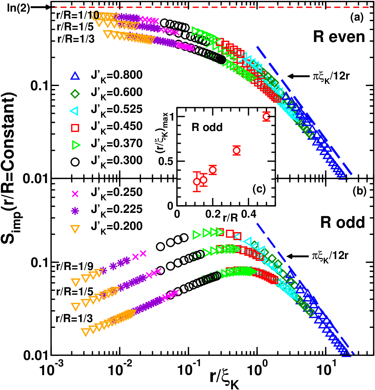
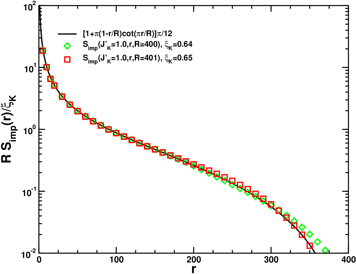
These results can be understood heuristically from a resonating valence bond picture of the ground spin in the Kondo spin chain model. Let’s first consider the case of integer total spin, even. Then the ground state is a spin singlet. It is important to realize that when the singlet ground state becomes degenerate with a triplet state. This occurs since the ground state of the other sites, has spin-1/2, as does the impurity spin and the two are coupled. However, by continuity in , it is the singlet state which is considered. This singlet state has strong entanglement of the impurity spin with the rest of the system, despite the fact that there is no term in the Hamiltonian coupling them together when . Any singlet state, and hence the ground state for any value of , can be written as some linear combination of “valence bond states” i.e. states in which pairs of spins form a singlet. (We can always restrict to “non-crossing” states such that if we draw lines connecting every pair of contracted spins, none of these lines cross each other.) If we consider a “frozen” valence bond state, i.e. any particular basis state, then the entanglement entropy is simply times the number of valence bonds from region to . There will always be a valence bond connecting the impurity spin to some other spin in the system; we refer to this as the Impurity Valence Bond (IVB). Intuitively, if the IVB connects the impurity to a spin outside of region A then we think of this as resulting in an impurity entanglement of ; however this picture is certainly naive because the valence bond basis, while complete, is not orthogonal. We may think of the typical length of the IVB as being since the spin screening the impurity is precisely the one forming the IVB. This picture makes it quite clear why is a decreasing function of and why is the characteristic scale for its variation.
Now consider the case of half-integer spin, odd. In this case, when there is zero entanglement between the impurity spin and the rest of the system. In this case the other sites have a spin zero ground state, decoupled from the impurity, which is unpaired. For odd and any the ground state always has spin 1/2. This can again be represented as an RVB state but each basis valence bond state has precisely one unpaired spin, which may or may not be the impurity. At is is the impurity with probability 1, but consider what happens as we increase from zero, corresponding to decreasing from infinity. The probability of having an IVB increases. On the other hand, the typical length of the IVB when it is present is which decreases. These two effects trade off to give a peak in when is approximately .
Our most important conclusion is probably that quantum impurity entanglement entropy appears to exihibit universal cross over between boundary RG fixed points with the size, , of region acting as an infrared cut-off.
VI Y-junctions of quantum wires
Now I consider 3 semi-infinite spinless Luttinger liquid quantum wires, all with the same Luttinger parameter, , meeting at a Y-junction,[46] as shown in Fig. (7). By imposing a magnetic field near the junction we can introduce a non-trivial phase, into the tunnelling terms between the 3 wires. A corresponding lattice model is:
| (198) |
(In general we can also introduce potential scattering terms at the end of each wire.) Here , , labels the 3 chains cylically so that we identify with . We bosonize, initially introducing a boson for each wire:
| (199) |
It follows immediately from the discussion of the 2-wire case in the 4th lecture that is irrelevant for , the case of repulsive interactions. Thus we expect the decoupled wire, zero conductance fixed point to be the stable one in that case. On the other hand, if the behaviour is considerably more complex and interesting. This case corresponds to effectively attractive interaction between electrons, as can arise from phonon exchange.

It is convenient to make a basis change, analgous to the even and odd channel introduce in Lecture 4 for the 2 wire junction:
| (200) |
and similarly for the ’s. It is also convenient to introduce 3 unit vectors, at angles with respect to each other, acting on the space:
| (201) |
We will also use 3 other unit vectors rotated by relative to these ones which we write as . The various boundary interactions are now written in this basis:
| (202) |
et cetera. Note that we have not yet imposed any particular BC’s on the fields at the origin. A more standard approach would probably be to start with the BC, = constant and then allow for the possibility that these BC’s renormalize due to the tunnelling. We call the current approach the method of “Delayed Evaluation of Boundary Conditions”. Hower, we expect the “centre of mass” field, is always pinned, constant. Since carries a non-zero total charge, and hence doesn’t appear in any of the boundary interactions, it would not make sense for any other type of boundary condition to occur in the “0” sector. We may thus simply drop the factor involving from all the boundary interactions; it makes no contribution to scaling dimensions. However, we must consider other possible BC’s in the , sector, since, for the simple D BC on is not stable, as mentioned above. Another simple possibility would be a D BC on : for two constants . To check the stability of this BC under the RG we must consider the LIO. The various candidates are the tunnelling and backscattering terms in Eq. (202). Imposing the BC constant, we can evaluate the scaling dimension of the exponential factors involving by the same method used in Lecture 4. The BC implies that we should replace by . The dimensions of these operators can then be read off:
| (203) |
et cetera. , for are the LIO’s. They are relevant for . Thus we see that this cannot be the stable fixed point for .
Stable fixed points, for can be identified from the form of the . If grows large under renormalization it is plausible that one or the other of this set of operators could develop an expectation value. Note that if:
| (204) |
this would correspond to strong tunnelling from to . On the other hand, if:
| (205) |
this would correspond to strong tunnelling from to . Breaking time reversal by adding a non-zero magnetic flux, , favours one or the other of these tunnelling paths, dependng on the sign of . On the other hand, in the time-reversal invariant case (or ) we do not expect such as expectation value to develop. These fixed points obey the BC’s:
| (206) |
for some constants . Note that since , these are only 2 independent BC’s. Introducing left and right moving fields:
| (207) |
we may write these BC’s as:
| (208) |
where is another constant vector and is a orthogonal matrix which we parameterize as:
| (209) |
with
| (210) |
We refer to these as the “chiral” fixed points, , with the or corresponding to the sign in Eqs. (206) and (210). Note that if we obtain the usual D BC on and if we obtain a D BC on . The chiral BC’s are, in a sense, intermediate between these other two BC’s.
As usual, we check their stability by calculating the scaling dimension of the LIO. Once we have the BC’s in the form of Eq. (208) it is straightforward to calculate the scaling dimension of any vertex operators of the general form:
| (211) |
| (212) |
Applying this formula to the fixed points we find that all the operators listed in Eq. (202) have the same dimension:
| (213) |
Since for , we conclude that the chiral fixed points are stable for this intermediate range of , only. Thus we hypothesize that the system renormalizes to these chiral fixed points for this range of whenever there is a non-zero flux, . However, these fixed points are presumably not allowed due to time reversal symmetry when and there must be some other stable fixed point to which the system renormalizes. This fixed point, which we referred to as “M” appears to be of a less trivial type than there “rotated D” states. An attractive possibility is that the M fixed point is destablized by an infinitesimal flux leading to a flow to one of the chiral fixed points. Alternatively, it is possible that there is a critial value of the flux, neccessary to destabilize the M fixed point. In that case there would presumably be two more, as yet undetermined, CI BC’s corresponding to these critical points.
VI.1 Conductance
Once we have identified the CIBC’s it is fairly straightforward to calculate the conductance using the Kubo formula. For a Y-junction the conductance is a tensor. If we apply voltages far from the junction on lead and let be the current, flowing towards the junction, on lead , then, for small ,
| (214) |
Since there must be no current when all the are equal to each other and since the total current flowing into the junction is always zero, it follows that
| (215) |
Also taking into account the symmetry of the model, we see that the most general possible form of is:
| (216) |
Here is the anti-symmetric, -symmetric tensor with . , which is odd under time reversal, can only be non-zero when there is a non-zero flux.
In the non-interacting case, in Eq. (198), , we may calculate the conductance by a simple generalization of the Landauer formalism. We imagine that the three leads are connected to distant reservoirs at chemical potentials . Each reservoir is assumed to emit a thermal distribution of electrons down the lead and to perfectly adsorb electrons heading towards it. The conductance can then be expressed in terms of the -matrix for the Y-junction. This is defined by solutions of the lattice Schroedinger equation:
| (217) |
The wave-functions are of the form:
| (218) |
for all and , , , with energy eigenvalues . The S-matrix is defined by:
| (219) |
The most general symmetric form is:
| (220) | |||||
In the time-reversal invariant case . It is then easy to see that unitarity of implies . In this case, for any wave-vector, , reaches for some value of of O(1). It can also be checked that when and , and . In this case an electron incident on lead is transmitted with unit probability to lead . To calculate the Landauer conductance, we observe that the total current on lead is the current emitted by reservoir , minus the reflected current plus the current transmitted from leads :
| (221) |
This gives the conductance tensor of the form of Eq. (216) with:
| (222) |
where are now evaluated at the Fermi energy. Thus the maximum possible value of ,in the zero flux case, is , when . On the other hand, for non-zero flux, when , , i.e. but . This implies that if a voltage is imposed on lead only, a current flows from lead to lead but zero current flows into lead . We refer to this as a prefectly chiral conductance tensor. Of course, if we reverse the sign of the flux then the chirality reverses with now inducing a current from lead to lead .
Now consider the conductance in the interacting case, for the three fixed points that we have identified. From the Kubo formula, we may write the DC linear conductance tensor as:
| (223) |
where . [At zero temperature, which I consider here, it is straightforward to take the zero frequency limit, in imaginary (Matsubara) formulation. At finite it is neccessary to do an analytic continuation to real frequency first.] We first transform from the basis to , inverting the transformation in Eq. (200):
| (224) |
makes no contribution to the conductance since always obeys a D BC as discussed above. Therefore:
| (225) |
where and the result is independent of . Here
| (226) |
To proceed we decompose:
| (227) |
The general type of BC of Eq. (208) allows us to regard the ,s as the analytic continuation of the ’s to the negative axis:
| (228) |
and thus
| (229) |
The Green’s function for is unaffected by the BC:
| (230) |
The integral in Eq. (223) gives:
| (231) |
Here is the Heavyside step function, often written but I avoid that notation here since has another meaning. Thus we obtain:
| (232) | |||||
Observing that and , since and are always positive in Eq. (223), we obtain:
| (233) |
For the D BC on , so:
| (234) |
corresponding to , . We observed above that this is a stable fixed point for , with . This exceeds the unitary bound on the conductance in the non-interacting case. An intuitive way of understanding why increasing leads to enhanced transmission is that attractive interactions can lead to pairing and either coherent pair tunnelling, or Andreev type processes (where an incident electron on one lead reflects as a hole while a pair is transmitted to a different lead) could lead to enhanced conductance.
We can now also obtain the conductance tensor for the chiral fixed points, which are stable for . Inserting Eqs. (209 and (210) in (233) we obtain:
| (235) |
For this reduces to the chiral conductance tensor discussed above in the non-interacting case with . However, for implying that a voltage on lead 1 not only leads to all current from 1 flowing to 2 but some additional current also flows from 3 to 2. Intuitively, we might think that, as the electrons pass from lead 1 to 2 they attract some electrons from lead 3. If our hypothesis, discussed above is correct that the zero flux “M” fixed point is unstable, then presumably an infinitesimal flux could lead to an RG flow to these stable chiral fixed points. Such a device would have an interesting switching property. Even a small magnetic field could switch the current completely from lead 2 to lead 3, at low enough temperatures and currents.
VII Boundary Condition Changing Operators and the X-ray Edge Singularity
There are some situations in condensed matter physics where we are interested in the response of a system to a sudden change in the Hamiltonian. A well-known example is the “X-ray edge singularity” in the adsorbtion intensity for X-rays in a metal, plotted versus X-ray energy. The X-ray dislodges an electron from a core level. This is assumed to suddenly switch on a localized impurity potential which acts on the conduction electrons. Since I have argued that quite generally the low energy properties of quantum impurity problems are described by CIBC’s we might expect that the low energy response to a sudden change in impurity interactions might be equivalent to the response to a sudden change in CIBC’s. Very fortunately, Cardy also developed a theory of BC changing operators which can be applied to this situation. In this lecture I will show how this theory can be applied to the usual X-ray edge problem and to a multi-channel Kondo version.[48]
VII.1 The X-Ray Edge Singularity
When an X-ray is adsorbed by a metal it can raise an electron from a deep core level, several keV below the Fermi surface, up to the conduction band. Let be this large energy difference between the Fermi energy and the core level and let be the energy of the X-ray. At , ignoring electron-electron interactions, this transition is only possible for . Here is a “renormalized” value of . I am assuming that the core level has a distinct energy, rather than itself being part of an energy band. This may be a reasonable approximation since core levels are assumed to be tightly bound to nuclei and to have very small tunnelling matrix elements to neighbouring nuclei. Presumably the excited electron will eventually relax back to the core level, possibly emitting phonons or electron-hole pairs. This is ignored in the usual treatment of X-ray edge singularities. Thus we are effectively ignoring the finite width of the excited electron states. Thus the X-ray adsorption intensity, will be strictly zero for , in this approximation. When the core electron is excited into the conduction band, it leaves behind a core hole, which interacts with all the electrons in the conduction band. Note that the only interaction being considered here is the one between the core hole and the conduction electrons. The X-ray edge singularity, at , in this approximation, is determined by the response of the conduction electrons to the sudden appearance of the core hole potential, at the instant that the X-ray is adsorbed. It turns out that, for only slightly larger then , very close to the threshold, is determined only by the conduction electron states very close to ; this fact allows us to apply low energy effective Hamiltonian methods. The difference between and arises from the energy shift of the filled Fermi sea due to the core hole potential. Not including the interaction with the external electromagnetic field, which I turn to momentarily, the Hamiltonian is simply:
| (236) |
where annihilates an electron in the core level at . I have assumed, for simplicity, that the core hole potential, , is a spherically symmetric -function. These assumptions can be easily relaxed. Following the same steps as in Sec. I, we can reduce the problem to a one-dimensional one, with left-movers only:
| (237) |
(I have set and .) It is convenient to bosonize. We may introduce a left-moving boson only:
| (238) |
| (239) |
The solubility of this model hinges on the fact that commutes with . Thus the Hilbert Space breaks up into two parts, in which the core level is either empty or occupied. The spectrum of the Hamiltonian, in each sector of the Hilbert Space, is basically trivial. In the sector where the core level is occupied, , we get the spectrum of free electrons with no impurity:
| (240) |
In the sector with we get the spectrum with a potential scatterer present:
| (241) |
What makes this problem somewhat non-trivial is that, to obtain the edge singularity, we must calculate the Green’s function of the operator which couples to the electromagnetic field associated with the X-rays: . This operator, which excites an electron from the core level into the conduction band, mixes the 2 sectors of the Hilbert Space. There is also some interest in calculating the Green’s function of the operator itself; this is associated with photo-emission processes in which the core electron is ejected from the metal by the X-ray. Again this operator mixes the two sectors of the Hilbert space.
In what may have been the first paper on bosonization, in 1969, Schotte and Schotte [47] observed that these Green’s functions can be calculated by taking advantage of the fact that the two Hamiltonians, and are related by a canoical transformation (and a shift of the ground state energy). To see this note that we may write in the form:
| (242) |
where:
| (243) |
Using the commutator:
| (244) |
we see that:
| (245) |
with the canonical transformation:
| (246) |
( can only be considered a unitary operator if we work in the extended Hilbert space which includes states with all possible BCs. maps whole sectors on the Hilbert space, with particular BCs, into each other.) Consider the core electron Green’s function, . We may write:
| (247) |
This is valid because, due to Fermi statistics, the core level must be vacant before acts, and occupied after it acts. i.e. we can replace the factor in by on the right hand side and by on the left. But and commute with so we have:
| (248) |
Here is the ground state of the system, including the core level and the conduction electrons. This state can be written: where is the state with the core level occupied and is the filled Fermi sea ground state of the conduction electrons, with no impurity potential. Using Eq. (245) we see that:
| (249) |
Using our explicit expression, Eq. (246) for , we have reduced the calculation to one involving only a free boson Green’s function:
| (250) |
Similarly, to get the Green’s function of I use:
| (251) |
and thus
| (252) | |||||
Finally, we Fourier transform to get the X-ray edge singularity:
| (253) |
This result is conventionally written in terms of a phase shift at the Fermi surface, rather than the potential strength, . The connection can be readily seen from Eq. (243) and the bosonization formula:
| (254) |
Since for represents the outgoing field, we see that:
| (255) |
where the phase shift is:
| (256) |
In fact, the parameter appearing in the bosonized Hamiltonian should be regarded as a renormalized one. Its physical meaning is the phase shift at the Fermi surface induced by the core hole. Only for small is it linearly related to the bare potential. Even if the core hole potential has a finite range, we expect the formulas for the X-ray edge singularity to still be correct, when expressed in terms of the phase shift at the Fermi surface, . More generally, if the core hole potential is not a -function, but is still spherically symmetric, a similar expression arises for the X-ray edge singularity with the exponent involving a sum over phase shifts at the Fermi surface, , in all angular momentum channels, .
The connection with a boundary condition changing operator (BCCO)[18, 19] is now fairly evident. If we revert to the formulation of the model on the semi-infinite line, , then the boundary condition is:
| (257) |
The operator, or , which creates the core hole potential in the Hamiltonian can be viewed as changing the boundary condition, by changing the phase shift . It is interesting to consider the relationship between the finite size spectrum with various BC’s and the scaling dimensions of and . We consider the system on a line of length with a fixed BC at the far end. Equivalently, in the purely left-moving formulation, for we have anti-periodic BC’s on a circle of circumference : . This corresponds to periodic BC’s on the left-moving boson field,
| (258) |
The mode expansion is:
| (259) |
The finite size spectrum is:
| (260) |
The universal ground state energy term, has been included. We see that can be identified with the charge of the state (measured relative to the filled Fermi sea). There is a one to one correspondance between the states in the FSS with excitation energy and operators with dimension in the free fermion theory. For example, corresponds to and respectively, of dimension . If we impose the “same” BC at both ends:
| (261) |
then this corresponds to the same anti-periodic BC on in the purely left-moving formulation, so the spectrum is unchanged. On the other hand if the phase shift is inserted at only, then , corresponding to:
| (262) |
corresponding to the replacement in Eq. (259). The FSS is now modified to:
| (263) |
In particular, the change in ground state energy due to the phase shift is:
| (264) |
Actually, adding the potential scattering also changes the ground state energy by a non-universal term, of O(1) which was adsorbed into in the above discussion. It is the term of O( which is universal and determines scaling exponents. The corresponding scaling dimension, is precisely the scaling dimension of the BCCO (or ). The energy of the excited state with obeys:
| (265) |
The corresponding scaling dimension, , is the scaling dimension of .
This is all in accord with Cardy’s general theory of BCCO’s. An operator which changes the BC’s from to generally has a scaling dimension, , which gives the ground state energy on a finite strip of length with BC’s at one end of the strip and at the other end, measured relative to the absolute ground state energy with the same BC’s , at both ends. This follows by making a conformal transformation from the semi-infinite plane to the finite strip. Explicity, consider acting with a primary BCCO at time at the edge, of a semi-infinite plane. Assume changes the BC’s from to . Then at time change the BC’s back to with the hermitean conjugate operator , also acting at , as shown in Fig. (8). Then the Green’s function on the semi-infinite plane is:
| (266) |
where is the scaling dimension of . Now we make a conformal transformation from the semi-infinite plane, , () to the finite width strip: , :
| (267) |
Note that the positive real axis, , , maps onto the bottom of the strip, . Choosing , , both points map onto the bottom of the strip. Note that, on the strip, the BC’s are at all times at the upper boundary, but change from to and then back to on the lower strip, at times , . The Green’s function on the strip is given by:
| (268) |
Here denotes the ground state of the system on the strip of length with the same BC, , at both ends of the strip. We may insert a complete set of states:
| (269) |
However the states must all be states in the Hilbert Space with different BC’s at and at . The corresponding energies, are the energies of the states with these different BC’s measured relative to the absolute ground state energy with the same BC’s at both ends. Taking the limit of large in Eqs. (268) and (269) we see that
| (270) |
where is the lowest energy state with BC’s and produced by the primary operator . The lowest dimension BCCO will simply produce the ground state with BC’s and . This corresponds to the operator in the X-ray edge model. On the other hand, the lowest energy state produced could be an excited state with BC’s and as in the example of , which produces the primary excited state with and BC’s twisted by the phase .

VII.2 X-ray Edge Singularites and the Kondo Model
This BCCO approach has various other applications [48] that go beyond the Schotte and Schotte results. One of them is to the Kondo model. So far we have been ignoring electron spin. If the core level is doubly occupied in the ground state, then it would have spin-1/2 after one electron is ejected from it by the X-ray. An initially spin-0 ion would then acquire a net spin-1/2. In addition to the potential-scattering interaction with the localized core hole, there would also be a Kondo interaction. Thus, it is interesting to consider the effect of suddenly turning on a Kondo interaction. We might expect that the Kondo effect could dominate the X-ray edge exponent, at least at low enough temperatures and frequencies: . Thus, we consider the Hamiltonian:
| (271) |
Now creates a core electron with spin and we have considered the general case of channels of conduction electrons, , , , Again we are interested in Green’s functions for the core electron operator, and also the operators . These Green’s functions should exhibit a non-trivial cross-over with frequency, or time, but at long times (frequencies very close to the threshold) we expect to be able to calculate them using properties of the Kondo fixed point. Since the operator creates the impurity spin, thus turning on the Kondo effect, it is again a BCCO. In this case, it should switch the BC from free to Kondo. Thus we expect its infrared scaling dimension to be given by the energy of the ground state with a free BC at one end of the finite system and a Kondo BC at the other. This spectrum is given by fusion with the primary in the spin sector. The ground state with these BC’s is always the primary itself, of dimension
| (272) |
This follows because the free spectrum includes the charge zero, spin flavour singlet, . Fusion with the spin primary always gives among other operators. This appears to have the lowest dimension of all fusion products. Note that this operator does not occur in the operator spectrum considered earlier at the Kondo fixed point. There we only considered operators produced by double fusion, corresponding to the FSS with Kondo BC’s at both ends of the finite system. This gives the operator spectrum with a fixed, Kondo BC. But for the Kondo X-ray problem, we must consider the corresponding BCCO. In general, for a CIBC obtained by fusion with some operator from a non-interacting BC, we may expect that the BCCO will be itself. We may check this result by a more elementary method in the single channel case. There the Kondo fixed point is equivalent to a phase shift of magnitude for both spin up and spin down, . The energy of this state, from Eq. (264) is simply implying a dimension . This agrees with Eq. (272) in the special case . We may also consider the dimensions of the operators . This operator has (one extra electron added to the conduction band), transforms under the fundamental representation of flavour, of dimension and has spin either or depending on how we sum over the spin indices and . The free spectrum always contains the operator corresponding to the fermion field itself, (where now denotes the -dimensional fundamental representation of ) and fusion with gives for all and for . These operators have dimension:
| (273) |
(It can be seen than corresponding to the free fermion operator.) Again we may check the case by more elementary arguments. We may find the unitary operators corresponding to as:
| (274) |
where we have introduced separate bosons for spin up and spin down electrons. , can depend on . It is convenient to switch to charge and spin bosons,
| (275) |
By choosing for and for we obtain:
| (276) |
These have the correct quantum numbers as can be seen by comparing with the standard bosonization formula for :
| (277) |
can be identified with the chiral component of the WZW model fundamental field. We then see that the spin singlet operator, , has in agreement with Eq. (273). On the other hand, the triplet operators have dimension . Since there is no primary for they contain Kac-Moody descendents, i.e. the spin current operator.
VIII Conclusions
Apart from the examples discussed in these lectures, BCFT techniques have been applied to a number of other quantum impurity problems, including the following. We can consider a local cluster of impurities. At distances large compared to the separation between the impurities the same methods can be applied. The 2-impurity Kondo model exhibits a NFL fixed point which can be obtained[49] by a conformal embedding which includes an Ising sector in which the fusion is performed. The 3-impurity Kondo model also exhibits a novel NFL fixed point. It was obtained[50] by a different conformal embedding with fusion in a parafermion CFT sector. Impurities in spin chains[51] and quantum Brownian motion[52] were also solved by these techniques. They were even applied[53] to a high energy physics model associated with Callan and Rubukaov. This describes a super-heavy magnetic monopole interacting with -flavours of effectively massless fermions (quarks and leptons). The monopole is actually a dyon having a set of electric charge states as well as a magnetic charge. When the fermions scatter off the dyon they can exchange electric charge. In this case fusion takes place in the charge sector.
The assumption that essentially arbitrary impurity interactions, possibly involving localized impurity degrees of freedom, interacting with a gapless continuum, renormalizes at low energies to a CIBC has worked in numerous examples. It appears to be generally valid and will likely find many other applications in the future.
IX Ackowledgements
I would like to thank my collaborators in the work discussed here, including: Andreas Ludwig, Sebastian Eggert, Masaki Oshikawa, Claudio Chamon, Ming-Shyang Chang, Erik Sorensen and Nicolas Laflorencie.
References
- [1] Lectures given at the Les Houches summer school, “Exact Methods in Low-dimensional Statistical Physics and Quantum Computing”, July, 2008.
- [2] See, for example, S.-K. Ma, Modern Theory of Critical Phenomena [Benjamin-Cummings, Reading, MA, 1976].
- [3] See, for example, the RG treatment of Landau Fermi Liquid Theory in R. Shankar, Rev. Mod. Phys. 66, 129 (1994).
- [4] I. Affleck, Fields, Strings and Critical Phenomena, p. 563-640, (ed. E. Brézin and J. Zinn-Justin North-Holland, Amsterdam, 1990).
- [5] T. Giamarchi, “Quantum Physics in One Dimension”, (Oxford, 2004).
- [6] I. Affleck, “Conformal Field Theory Approach to the Kondo Effect”, Acta Phys.Polon. B26 (1995) 1869, cond-mat/9512099.
- [7] J. Kondo, Prog. Theor. Phys. 32, 37 (1964).
- [8] A. Hewson, “The Kondo Model to Heavy Fermions”, (Cambridge, 1997).
- [9] I. Affleck and A.W.W. Ludwig, Nucl. Phys. B360, 641(1991) .
- [10] V. Barzykin and I. Affleck, Phys. Rev. B57, 432 (1998).
- [11] P.W. Anderson, J. Phys. C3, 2346 (1970).
- [12] K.G. Wilson, Rev. Mod. Phys. 47, 773 (1975).
- [13] P. Nozières, Proc. of 14th Int. Conf. on Low Temp. Phys. [ Ed. M. Krusius and M. Vuorio ] V.5, P.339, (1975).
- [14] N. Andrei, Phys. Rev. Lett. 45, 379 (1980).
- [15] P.B. Weigmann, Sov. Phys. J.E.T.P. Lett. 31, 392 (1980).
- [16] R. Bulla, T.A. Costi and Th. Pruschke, Rev. Mod. Phys. 80, 395 (2008).
- [17] P. Nozières and A. Blandin, J. de Physique, 41, 193 (1980).
- [18] J.L. Cardy, proceedings of Les Houches summer school, 2008.
- [19] J.L. Cardy, Nuc. Phys. B324, 581 (1989).
- [20] E. Witten, Commun. Math. Phys. 92, 455 (1984).
- [21] J.L. Cardy and D. Lewellen, Phys. Lett. B259, 274 (1991).
- [22] V.G. Knizhnik and A.B. Zamolodchikov, Nucl. Phys. B247, 83 (1984).
- [23] P. Di Francesco, P. Mathieu and D. Senechal, Conformal Field Theory, (Springer-Verlage, New York, 1997).
- [24] D. Gepner and E. Witten, Nucl. Phys. B278, 493 (1986).
- [25] A.M. Tsvelick, J. Phys. C18, 159 (1985).
- [26] A.B. Zamolodchikov, Pis’ma Zh. Eksp. Teor. Fiz. 43, 565 (1986) [J.E.T.P. Lett. 43, 730 (1986)].
- [27] D. Friedan and A. Konechny, Phys. Rev. Lett. 93, 030402 (2004).
- [28] V.G. Kac and K. Peterson, Adv. Math. 53, 125 (1984).
- [29] I. Affleck and A.W.W. Ludwig, Phys. Rev. B48, 7297 (1993).
- [30] Y. Oreg and D. Goldhaber-Gordon, Phys. Rev. Lett. 90, 136602 (2003).
- [31] I. Affleck, A.W.W. Ludwig, H-B. Pang and D. L. Cox, Phys. Rev. B45, 7918 (1992).
- [32] M. Pustilnik, L. Borda, L. Glazman and J. von Delft, Phys. Rev. B 69, 115316 (2004).
- [33] R. M. Potok, I. G. Rau, Hadas Shtrikman, Yuval Oreg, D. Goldhaber-Gordon, Nature 446, 167 (2007).
- [34] S. Eggert and I. Affleck, Phys. Rev. B46, 10866 (1992).
- [35] C.L. Kane and M.P.A. Fisher, Phys. Rev. B46, 15233 (1992).
- [36] A.B. Zamalodchikov and S. Ghoshal, Int. J. Mod. Phys. A9 3841 (1994).
- [37] S. Tarucha, T. Honda and T. Saku, Sol. St. Comm. 94, 413 (1995).
- [38] D.L. Maslov and M. Stone, Phys. Rev. B52, R5539 (1995); V.V. Ponomarenko, ibid, 52, R8666; I. Safi and H.J. Schulz, ibid R17040 (1995); C. Chamon and E. Fradkin, ibid 56, 2012 (1997); K.-I. Imura, K.-V. Pham, P. Lederer and F. Piechon, ibid 66, 035313 (2002).
- [39] K. Moon, H. Yi, C.L. Kane, S.M. Girvin and M.P.A. Fisher, Phys. Rev. Lett. 71, 4381 (1993).
- [40] P. Fendley, A. W. Ludwig, and H. Saleur, Phys. Rev. Lett. 74, 3005 (1995).
- [41] N. Laflorencie, E.S. Sorensen and I. Affleck, J Stat Mech. (2008) P02007.
- [42] R.G. Pereira, N. Laflorencie, I. Affleck and B.I. Halperin, Phys. Rev. B 77, 125327 (2008).
- [43] E.S. Sorensen, M.-C. Chang, N. Laflorencie, and I. Affleck, J. Stat. Mech. P08003 (2007).
- [44] P. Calabrese and J.L. Cardy, J. Stat. Mech. 04010 (2004).
- [45] C. Holzhey, F. Larsen and F. Wilczek, Nucl. Phys. B 424, 443 (1994).
- [46] M. Oshikawa, C. Chamon and I. Affleck, J Stat Mech. P02008, 102 (2006).
- [47] K.D. Schotte and U. Schotte, Phys. Rev. 182, 479 (1969).
- [48] I. Affleck and A.W.W. Ludwig, J. Phys. A27, 5375 (1994).
- [49] I. Affleck, A.W.W. Ludwig and B.A. Jones, Phys. Rev. B52, 9528 (1995).
- [50] K. Ingersent, A.W.W. Ludwig and I. Affleck, Phys. Rev. Lett. 95, 257204 (2005).
- [51] I. Affleck, M. Oshikawa and H. Saleur, J. Phys. A34, 1073 (2001).
- [52] I. Affleck, M. Oshikawa and H. Saleur, Nucl. Phys. B594, 535 (2001).
- [53] I. Affleck and J. Sagi, Nuc. Phys. B417, 374 (1994).