Sersiclets – A Matched Filter Extension of Shapelets for Weak Lensing Studies
Abstract
The precision study of dark matter using weak lensing by large scale structure is strongly constrained by the accuracy with which one can measure galaxy shapes. Several methods have been devised but none have demonstrated the ability to reach the level of precision required by future weak lensing surveys. In this paper we explore new avenues to the existing Shapelets approach, combining a priori knowledge of the galaxy profile with the power of orthogonal basis function decomposition. This paper discusses the new issues raised by this matched filter approach and proposes promising alternatives to shape measurement techniques. In particular it appears that the use of a matched filter (e.g. Sérsic profile) restricted to elliptical radial fitting functions resolves several well known Shapelet issues.
Keywords:
Cosmology – dark matter: gravitational lensing.1 Introduction
Galaxy shapes provide the unique signature of gravitational lensing by large scale structure, which has been recognized as a key to the study of dark matter and dark energy (Munshi et al., 2008). A limiting factor is the accuracy with which one can measure shapes (Heymans et al., 2006; Massey et al., 2007; Hoekstra & Jain, 2008). Among the different existing methods, one particularly interesting approach is the decomposition of galaxy images using basis functions e.g. Bernstein & Jarvis (2002) or Shapelets (Refregier, 2003; Refregier & Bacon, 2003; Massey & Refregier, 2005). The strengths of this approach rely on the fact that the shape measurement is analytical and therefore time efficient as it involves rather small matrix multiplications. Shapelets decompose an image into a linear combination of orthonormal components up to some truncation order, and the shape parameters are extracted from a least-squares best fit using the recomposed (noise free) model. However, the Shapelet type approach suffers from a few difficulties:
(i) The choice of the decomposition truncation order is arbitrary. In practice, different lensing groups use radically different “optimal” truncation orders. Some prefer low (Kuijken, 2006), while others prefer high (Bergé et al., 2008), although the values for different truncation order could be very different. Therefore a constant criterion to measure the shape does not appear to be a robust guarantee of unbiased shape measurement.
(ii) “Easy cases” such as large and bright elliptical galaxies are poorly fitted. This suggests that a good fit for low signal-to-noise galaxies does not necessarily mean that the shape has been correctly measured, since it could just be buried in the sky noise. This is the overfitting problem.
(iii) Basis decomposition has too many degrees of freedom for shear measurement, since ideally we are only interested in two numbers (or six if we include the flexion). This is where galaxy morphology and shear measurement are clearly two different problems.
All of those problems have one common origin, namely the choice of the zeroth order weight function – Gaussian functions for both Cartesian (Refregier, 2003) and Polar Shapelets (Massey & Refregier, 2005), as well as Bernstein & Jarvis (2002). Unfortunately, Gaussian functions are poor matches to real galaxy profiles. Ideally, we would like the zeroth order to be as close as possible to the real profile, and leave to the basis decomposition the task to fit departures from this “typical” profile.
Currently the most promising shape measurement method uses a bayesian model fitting approach (Miller et al., 2007; Kitching et al., 2008). This method does not suffer from the same issues as Shapelets, but is limited by the strong galaxy profile prior.
In this paper, we investigate how the change of the weight function affects the basis decomposition method, and how it leads naturally to a hybrid method which combines Shapelets and fitting techniques. We choose to focus on the Sérsic profile (hence the term Sersiclets), but our discussion can be extended to any profile11 1 While working on the concepts discussed in this paper, we became aware of similar investigations using exponential and hyperbolic sech functions (Kuijken & van Uitert in prep)., e.g. Moffat profile for ground based point spread function (PSF). Section 2 introduces the notation and gives a technical description of the new fitting functions. Section 3 shows the impact of those fitting functions on shape fitting and decomposition. Finally, Section 4 summarizes our work so far and future possibilities.
Note that in this paper we choose not to discuss the PSF deconvolution. Indeed, the problems we mentioned earlier affect equally the measurement of galaxy shapes whether or not the galaxies are convolved with a PSF, and Shapelets are a popular approach because their Gaussian properties allow for very efficient PSF treatment. The PSF deconvolution issue goes beyond this work because it depends on how the PSF is measured and interpolated between stars. Moreover the approach developed here could as well be applied to the PSF profile measurement separately, and then used later to address the deconvolution step through a forward convolution model fitting method. See for example Kitching et al. (2008).
2 Methodology
2.1 Basis functions in polar coordinates
In 1D, all polynomials of degree are orthonormal with respect to a weight function if they satisfy
| (1) |
A particular choice of weight function uniquely determines the family of polynomials (e.g. for the Cartesian Shapelets, a Gaussian weight defines the Hermite polynomials). A complete set of polynomials can be useful for decomposing an arbitrary function as a linear combination of basis functions such that
| (2) |
In 2D, the basis functions can be represented using polar coordinates. Following the intuition for Polar Shapelets, we separate our basis functions into the radial component and the angular component . We also assume that the weight function has no angular dependence. The 2D basis functions in polar coordinates would be in the form
| (3) |
The orthonormality is then written as
| (4) |
where * denotes complex conjugate. The orthonormality requirements for radial and angular parts, and , can be satisfied independently. In particular, is an orthonormal polynomial of degree with respect to the weight function . The integration limit for the radial component will be discussed in Section 2.4.
With an orthogonal and complete set of basis functions, an arbitrary image can then be decomposed into
| (5) |
where the complex basis coefficients satisfy so that is wholly real. We will refer as “order” in the following sections.
Readers familiar with Polar Shapelets may notice that our radial component here only requires , and increases in steps of 1. In Polar Shapelets, the radial component requires both and , and increases in steps of 2. Our choice to completely decouple the radial and the angular components is of mere convenience, which comes with the cost that our set of “basis functions” is no longer complete. Consequently, our set of fitting functions cannot decompose an arbitrary image. As we shall see in Section 2.5 and Section 2.6, though, the lack of completeness is not a hindrance to decomposing images of galaxies for weak lensing, as galaxies follow Sérsic profiles (Sérsic, 1968) and are not arbitrary in general.
2.2 Weight function
The basis functions in Shapelets often require high order polynomials to describe galaxy shapes accurately because galaxies’ radial light profiles do not match the weight functions. Galaxies’ light profiles are well described by Sérsic’s empirical formula (Peng et al., 2002):
| (6) |
where is a scale radius, and is known as the Sérsic index. For , . We use a parameterized form of Equation 6 as our weight function:
| (7) |
2.3 Radial component
The radial component involves a non-trivial computational step, as must satisfy the orthonormality requirement described in Section 2.1. We obtain by the Gram-Schmidt process22 2 http://mathworld.wolfram.com/Gram-SchmidtOrthonormalization.html. Using Dirac notation , the Gram-Schmidt process generates each by a recurrence relation:
where , and . After the recurrence step, each is individually normalized.
2.4 Integration limits
When generating the radial polynomials (Section 2.3), a sensible integration limit must be chosen. In Shapelets one can integrate from 0 to thanks to the Gaussian function’s localized profile. For Sérsic functions in general, however, the profile may not be localized enough to allow for an infinitely large domain. This is generally true for any galaxy and stellar profile used as a weight function.
The problem with using an infinitely large domain is the lack of mutual independence among the fitting functions. In order to construct a model as a linear combination of fitting functions, each fitting function must be distinct so that there is no redundancy in their shapes. Figure 1 shows the polynomials that are generated using a weight function (Equation 7) with . We find that limiting the orthogonality to a finite domain preserves linear independency better than extending to an infinitely large domain.
We conveniently choose for our domain. For a square image stamp of pixels, would be normalized to have units of pixels. It also allows us to constrain , as the scale radius is always positive, and a galaxy should be well captured in a stamp.


2.5 Completeness
Although the fitting functions of Sersiclets are indeed mutually orthonormal, they are not necessarily complete. As a result, Equation 5 does not necessarily converge, even at high . The basis functions in both Cartesian and Polar Shapelets are complete, meaning that Equation 5 can converge for any arbitrary as .
The incompleteness of Sersiclets is shown in Figure 2. It shows the average difference squared per pixel when decomposing a noiseless elliptical object on a grid by integrating Equation 5 with , and exploiting orthonormality to obtain each . The reconstruction using Sersiclets does not improve even as the order increases; in fact, the reconstruction becomes slightly worse because higher order contributions are as small as the discretization error. Clearly, Sersiclets fail to decompose even a simple elliptical object.
For this reason, we would not attempt the decomposition by including higher order fitting functions. In the next section we take a different approach – throwing away all circularly asymmetric components. The lack of contribution by those components is an important rationale of our technique to reduce the set of fitting functions.

2.6 Fitting set reduction
It is clear from Section 2.5 that the fitting set should be reduced in order to take advantage of the matched filter due to the lack of completeness. In the following we reduce our set of fitting functions to only the circularly symmetric components (), and we introduce ellipticities by transforming the now perfectly circular model by “scaling” and “rotating”, which yield unique values of and . This is similar to the process described in Bernstein & Jarvis (2002).
The set of “reduced Sersiclets” has two advantages; eliminating the components not only cures the overfitting problem, but it also offers a dramatic increase in speed as the number of terms in Equation 5 now increases like rather than . It also provides a direct estimate of and , which are treated as asymmetric scaling parameters for the fitting function.
We focus on fitting profiles that are smooth, centrally peaked, and elliptical in general. These fitting functions are not suitable for studying galaxy morphology, as they cannot provide information about a galaxy’s detailed structure. In weak gravitational lensing studies, however, the details in the typical faint images analyzed are dominated by noise and should not be fitted. Therefore our reduced fitting set offers a natural regularization process which is missing in the standard Shapelet approach. Our method is a hybrid of Shapelets and fitting techniques, where we do allow some decomposition into fitting functions, but those fitting functions are by construction axisymmetric and therefore prevent isophote mixing (i.e. overfitting) as higher order fitting techniques do.
3 Experiment
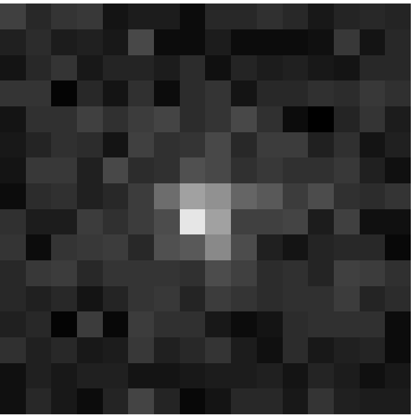
Our experiment at this stage is not a rigorous test for shape measurement, as our test cases (Figure 3) are idealized profiles without PSF convolution. Rather, we are exploring the effect of using a variety of weight functions with different (, ). Our test cases consist of both circular and elliptical profiles. We generated two-dimensional reduced maps of vs order at fixed values.
The maps are then compared against those generated using Polar Shapelets, which we will refer to simply as “Shapelets” in the following discussion. In Shapelets’ case, the coordinate is also normalized to . The “scaling-factor” in Shapelets is now comparable to in Sersiclets, which is relative to the size of the image. The model fits for both Sersiclets and Shapelets were computed using Hrothgar33 3 http://hrothgar.sourceforge.net/ implemented in C.
 |
 |
 |
| de Vaucouleurs | exponential | generic Sérsic |
 |
 |
 |
| exponential | exponential | generic Sérsic |
3.1 Results – Circular models using the full fitting set
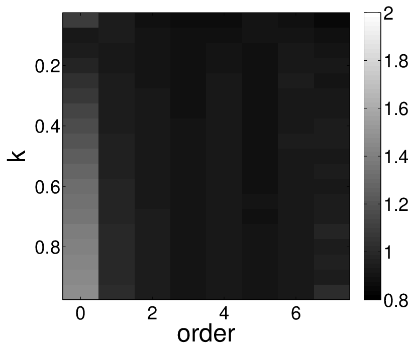
We first test the full fitting set by fitting against circular profiles. In Figure 4, we see that convergence of is achieved very quickly. This is not surprising as the weight functions in the models are indeed realistic. More importantly, we find that the fits are insensitive to the choice of after the first few orders. This robustness allows us to obtain good fits without searching for an optimal . This result is useful in fitting large collections of objects, where families of objects can simply share the same pair of without compromise.
Comparing the maps and image reconstructions between Sersiclets and Shapelets reveals Sersiclets’ advantage. In very non-Gaussian cases such as the de Vaucouleurs case, Sersiclets converge at a much lower order than Shapelets. In fact, Shapelets require low signal-to-noise ratios in order to render an illusion of “good fit”. From Figure 4, we see that Shapelets’ lowest order best fit at already shows signs of noise fitting; the model is not smooth, and it shows non-circular isophotes. Sersiclets, though, can recover the smooth and circular profile at orders 0 or 1.
| Sersiclets | Shapelets |
|---|---|
 |
 |
 |
 |
3.2 Results – Elliptical model using the reduced fitting set
For the elliptical profiles, the maps (Figure 5) are very similar to those shown in Figure 4. This means that the components were indeed not important, and Sersiclets’ robustness in are preserved. Fitting set reduction as described in Section 2.6 has been done to both Sersiclets and Shapelets. In Shapelets’ case, since components do not exist for odd orders, only even orders were possible. As seen in the image reconstruction in Figure 5, the Shapelet fit no longer shows noise fitting thanks to fitting set reduction.
The residuals of measured values corresponding to each input value have been plotted in Figure 6. It is clear that as the fit improves with higher orders, the scatter in the measured ellipticity is reduced. For Shapelets, the solution does not show robustness in as the measured ellipticities are more scattered than the Sersiclets’ case.
| Sersiclets | Shapelets |
|---|---|
 |
 |
 |
 |


| 0.130 | 0.225 | 0.43 | 1.0 |
|---|---|---|---|
| 0.244 | 0.089 | 0.43 | 1.0 |
| 0.180 | 0.186 | 0.43 | 1.0 |
| 0.164 | 0.24 | 1.0 | |
| 0.274 | 0.146 | 0.24 | 1.0 |
| 0.011 | 0.310 | 0.24 | 1.0 |
| 0.012 | 0.069 | 0.29 | 0.75 |
| 0.066 | 0.024 | 0.29 | 0.75 |
| 0.024 | 0.29 | 0.75 | |
| 0.348 | 0.28 | 0.75 | |
| 0.116 | 0.357 | 0.28 | 0.75 |
| 0.28 | 0.75 |
3.3 Discussion
Sersiclets’ robustness in and its ability to converge in relatively low orders comes from the abundance of its degrees of freedom in the model. For the full fitting set, Equation 5 has terms in the summation as the angular quantum number increases in steps of 1. Polar Shapelets, however, have only terms as increases in steps of 2 at a given order of . For the reduced fitting set, Sersiclets have terms, and Polar Shapelets have only terms. Together with and , Sersiclets would have about twice as many degrees of freedom as Polar Shapelets. To facilitate a fair comparison, Figure 6 compares Sersiclets at order 3 against Shapelets at order 6 in the second and third panels. This ensures that the test uses the same degrees of polynomials available to each decomposition technique.
A drawback of Sersiclets is numerical instability. Hermite or associated Laguerre polynomials in Shapelets can be generated very easily with elementary operations, whereas the general Sersiclet polynomials require gamma functions. In particular, the analytical solution to the integral
| (8) |
which is ubiquitous in Section 2.3, can be written as
| (9) |
where and are the complete and incomplete gamma functions, respectively, and as before. At first glance, it may be tempting to use the analytical solution because it exists and gamma functions can be readily evaluated. Upon closer inspection, though, Equation 9 evaluates the difference between two gamma functions, each on the order of . The difference is then scaled by a number raised to the power of . One needs to be careful when evaluating such an expression if becomes large, especially when using numerical libraries with single precision. Alternatively, the integrand in Equation 8 is a smooth function, so the integral can be evaluated directly without implementing the analytical solution.
Sersiclets can be generalized to different weight functions. In our derivation, although we have chosen the Sérsic function as our weight function, the process would still be the same for any weight functions which are intrinsically elliptical without explicit angular dependence. This allows for modeling different types of objects such as the PSF using the Moffat profile as the weight function. The integration limit of the radial component, as we discussed in Section 2.4, can be either finite or infinite depending on whether the weight function is sufficiently localized.
4 Conclusion
We presented an extension of Shapelets by using an arbitrary weight function in place of the Gaussian function. As galaxies’ light profiles follow the Sérsic profile on average, we used the Sérsic function as our weight function. This allowed us to fit cuspy galaxies at lower orders than Shapelets could.
Because the Sérsic function lacks analytical properties, we used the Gram-Schmidt process to generate the orthonormal polynomials as radial components for the fitting functions, where the integrals in the process must be evaluated numerically. As the Sérsic profile has poor local support, the integration limit must be truncated to a finite limit.
We found that the full set of fitting functions for Sersiclets cannot decompose an arbitrary image even at high orders, as the fitting functions do not form a complete set. Instead of modeling objects using all fitting functions, we reduced the fitting set to only the circularly symmetric components (). The model was then sheared by and to render elliptical shapes. The reduced set of fitting functions defines a hybrid method which combines the most interesting features of the basis decomposition and the fitting technique.
Our experiments so far only focused on idealized images simulated using known profiles and noise. Both the full and the reduced Sersiclets outperformed Shapelets, as we expected. The Shapelet matched filter’s true performance will be tested in a future paper on image simulations such as those for GREAT08 (Bridle et al., 2008). The C code to evaluate Sersiclet models is publicly available on request.
Acknowledgments
We are grateful to Ariel Zhitnitsky for inspiring discussions at the beginning of this work, and Peter Melchior for valuable comments. We also thank the anonymous referee for detailed and very constructive comments on the manuscript. Wayne Ngan, LVW, and Henk Hoekstra are supported by NSERC and CIfAR.
References
- Bergé et al. (2008) Bergé, J., Pacaud, F., et al., 2008, MNRAS, 385, 695.
- Bernstein & Jarvis (2002) Bernstein, G., Jarvis, M., 2002, AJ, 123, 583.
- Bridle et al. (2008) Bridle, S., et al., 2008, arXiv:0802.1214.
- Heymans et al. (2006) Heymans, C., Van Waerbeke, L., et al., 2006, MNRAS, 368, 1323.
- Hoekstra & Jain (2008) Hoekstra, H., Jain, B., 2008, arXiv:0805.0139.
- Kitching et al. (2008) Kitching, T., Miller, L., et al. 2008, arXiv:0802.1528.
- Kuijken (2006) Kuijken, K., 2006, A& A, 456, 827.
- Massey et al. (2007) Massey, R., Heymans, C., et al., 2007, MNRAS, 376, 13.
- Massey & Refregier (2005) Massey, R., Refregier, A., 2005, MNRAS, 359, 1277.
- Miller et al. (2007) Miller, L., Kitching, T., et al., 2007, MNRAS 382, 315.
- Munshi et al. (2008) Munshi, D., Valageas, P., et al., 2008, PhR, 462, 67.
- Peng et al. (2002) Peng, C., Ho, L., et al., AJ, 2002, 124, 266.
- Refregier (2003) Refregier, A., 2003, MNRAS, 338, 35.
- Refregier & Bacon (2003) Refregier, A., Bacon, D., 2003, MNRAS, 338, 48.
- Sérsic (1968) Sérsic J. L., 1968, Atlas de Galaxias Australes (Córdoba: Obs. Astron., Univ. Nac. Córdoba).