Creation-annihilation processes in the ensemble of constant particle number
Abstract
We study, in the ensemble of constant particle number, processes in which a cluster of particles is annihilated and particles are created catalytically in active sites. In this ensemble, particles belonging to a cluster of particles jump to distinct active sites. As examples of our prescription, we analyze numerically three nonequilibrium systems that annihilate cluster of particles that are identified as conserved versions of the pair annihilation contact model, triplet annihilation contact model and pair contact process. We show also how to set up the constant particle number ensemble from the constant rate ensemble.
PACS numbers: 05.70.Ln, 05.50.+q, 05.65.+b
I Introduction
The use of distinct ensembles in equilibrium statistical mechanics, in which systems are described by a given Hamiltonian, is a well established concept [1]. There is a standard procedure for passing from a given ensemble to another. For nonequilibrium systems [2], on the other hand, this procedure can not be used, since they are not described by a Hamiltonian and therefore, their probability distribution are not known a priori. In most cases nonequilibrium systems are defined in a constant rate ensemble, (which we call ordinary version), but the possibility of using another ensemble was put forward by Ziff and Brosillow [3] when they used a constant coverage ensemble in their study of an irreversible surface-reaction model. Subsequently, Tomé and de Oliveira [4] introduced the contact process in the ensemble of constant number of particles.
In the conserved contact process (CCP) [4], a particle chosen at random leaves its place and jumps to one of the many active sites of the lattice. The CCP displays properties that in the thermodynamic limit are identical to the ordinary contact process. Hilhorst and van Wijland [5] provided a proof of the equivalence between the constant rate and the constant particle number ensembles for the contact process. Later, de Oliveira [6] extended the proof for any reaction process that annihilate one particle [4, 7, 8]. Sometimes the use of the conserved version is more appropriate than the ordinary version as for example in the study of a first-order transition. This advantage has been exploited by Ziff and Brosillow [3], Loscar and Albano [9] that studied hysteretic effects in a model that describes the CO+NO reaction, and more recently by Fiore and de Oliveira [8].
Here, we analyze in the ensemble of constant particle number one-dimensional models whose ordinary versions have been previously studied. These models are: the pair-annihilation contact model (PAM) [10], the triplet-annihilation contact model (TAM) [10, 11], and the pair contact process (PCP) [12, 13, 14]. In these models, a cluster of particles is spontaneously annihilated and particles are catalytically created in active sites. Active sites are empty sites surrounded by a neighborhood of particles.
II TRANSITION RATES
Consider a site of regular lattice. To each site of the lattice we attach an occupation variable which takes the values or according whether the site is empty or occupied by a particle. In the constant rate ensemble, the usual process is composed of creation of a single particle (0 1) with transition rate , and annihilation of a cluster of particles in a row (111…1000…0) with transition rate . The transition rate is the probability per unit time of creating a particle at the site . The transition rate is the probability per unit time of annihilating a particle at the site . The total transition rate for these two reaction processes is given by
| (1) |
The quantities and will be defined according to the specific model and they depending on the local configuration of particles. The quantities and , which we call strengths of the annihilation and creation process, are parameters that gives the weight of each subprocess. Diffusion of particles consists of a particle hopping to its nearest neighbor. In diffusive models, the diffusion of particles and the reaction process occur with probability and , respectively.
In the ensemble of constant particle number, the jumping process and the diffusion of particles are chosen with probabilities and , respectively. In the hopping step, an occupied site and its nearest next neighbor interchange their occupation variables, whereas in the jumping step, adjacent particles leave their places and arrive at active sites. Thus, in the ensemble of constant particle number, both the creation and annihilation of particles are replaced by jumping process.
III EQUIVALENCE OF ENSEMBLES
In the construction of conserved models we have to be concerned only with the creation and annihilation processes since the diffusion process already conserves the particle number. In the case of processes that annihilate a pair of particles (PAM and PCP), the jumping process occurs with rate . In the case of annihilation of a triplet of neighboring particles (TAM), it occurs with rate .
To demonstrate that this conserved dynamics is equivalent to the ordinary dynamics described by Eq. (1) we follow the same reasoning given by de Oliveira [6]. Let us consider the specific case of models that annihilate two particles. In this case, two particles, belonging to the neighborhood of site , chosen at random, jump to two distinct active sites, and , also chosen at random. The jumping process occurs with rate where is the number of sites of the lattice. Let us evaluate the total rate in which particles leave the neighborhood of site . In the thermodynamic limit, the sums and approach, by the law of large numbers, the averages and , respectively. Therefore we have . Similarly, the total rate at which a particle arrives at the site is and the total rate at which a particle gets to the site is .
Comparing these results with the rate (1), we see that and should be proportional to and , respectively. Defining as the ratio , we can write the following relation
| (2) |
valid for any process that annihilates a pair of particles in the ensemble of constant particle number.
When we add a diffusive step, the ensembles are also equivalent, but the diffusion rate used in the constant rate ensemble will not have, in general, the same value of diffusion rate that is used in the constant particle number ensemble. A relation between the rates and is given by
| (3) |
where the factor comes from the ratio between the occurrences of diffusive process and the jumping process.
IV Pair-annihilation contact model
IV.1 Constant rate ensemble
In the ordinary PAM, the creation of particles is catalytic and a pair of particles is annihilated spontaneously. It is represented by the chemical reactions:
| (6) |
| (7) |
describing the catalytic creation and annihilation of a pair of particles, respectively. The rates and in Eq. (1) are given by
| (8) |
where the summation is over the nearest neighbor sites and
| (9) |
The strengths of the creation and annihilation processes are given by and .
For values of , the system is constrained into the absorbing state (without particles), whereas for we have an active state in which particles are created and pairs of neighboring particles are annihilated. A continuous phase transition between these two regimes occurs at [10]. Close to the critical point, the order parameter (here the density of particles ) follows a power law
| (10) |
where . The PAM is found to belong to the directed percolation universality class (DP) [2].
IV.2 Constant particle number ensemble
The Monte Carlo simulation of the conserved PAM is performed as follows. The jumping process and the diffusive process are chosen with probabilities and , respectively. If the jumping process is chosen, then a pair of neighboring particles is chosen at random. Next, we choose two empty sites each one surrounded by at least one particle. The two particles belonging to the selected pair jump to these two active sites. If the diffusive process is chosen, then a particle chosen randomly is moved to one of its neighboring site, provided it is empty. In this ensemble, the rate is evaluated by using formula (2), where the quantities and are given by Eqs. (8) and (9). To determine the critical rate we have simulated the conserved PAM in the subcritical regime. In this regime we have an infinite lattice and a finite particle number . The critical value is obtained by assuming the asymptotic relation
| (11) |
A linear extrapolation of versus gives , since when we have . The behavior of versus for the conserved PAM in the subcritical regime is shown in Fig. 1. In the limit of , we obtain , in excellent agreement with the value obtained from its ordinary version [10].

According to Vicsek [15], in the critical point, we have a formation of fractal clusters. To calculate the fractal dimension for a fixed , we have measured the maximum distance between two particles of the system as a function of the particle number .
Following Bröker and Grassberger [16], we assume the following asymptotic behavior
| (12) |
where is the fractal dimension. The fractal dimension is related to the survival probability exponent , the mean number of particles exponent , and the dynamic exponent by [2]. In Fig. 2 we show a log-log plot of versus for the conserved PAM for some values of the diffusion rate . The values of are consistent with the value , obtained for the CCP [7].

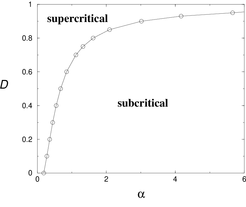
Using Eq. (11) we have built the phase diagram shown in Fig. 3 for several values of diffusion rate . Increasing the diffusion rate, we expect an increase in the value of , since by dispersing particles the density of pairs of neighboring particles decreases whereas the density of active sites increases. Our results show that for sufficiently rapid diffusion, , the critical value of increases without limit, that is, , in agreement with the results obtained by Dickman [10].
To determine the exponent , we have simulated the conserved PAM in the supercritical regime for some values of the diffusion rate . In this regime, the density is kept fixed for a size system . We have used a lattice with sites and a number of Monte Carlo steps ranging from to . The exponent is obtained from the log-log plot of versus as shown in the Fig. 4. We used the values of calculated by using the equation (11). For , we obtained that is in excellent agreement with the value obtained for the CCP [4]. The simulations performed at and give exponents also compatible with this value.

V Triplet-annihilation contact model
V.1 Constant rate ensemble
The ordinary TAM is composed of the creation of particles and annihilation of three neighboring particles. It is represented by the chemical reactions:
| (13) |
| (14) |
describing the catalytic creation and annihilation of a triplet of particles, respectively. The quantity is also given by Eq. (8) and the rate is given by
| (15) |
Without diffusion, a continuous phase transition to an absorbing state occurs at [10, 11] with critical exponent .
The competition between diffusion and reaction process may bring great changes in the phase diagram. For example, in the multiple-creation contact processes, the transition becomes first order for high enough values of diffusion [4, 8]. In the PCP, several works have reported a change in the universality class for nonzero values of diffusion rate. For the ordinary TAM, previous works [10, 11] have shown that in the presence of diffusion, the system exhibits a reentrant phase diagram as can be seen in Fig. 6.
In references [10, 11], the processes of diffusion, creation and annihilation are chosen with probabilities , and , respectively. To compare ordinary results with ours, it is necessary to convert the parameters. The relation between and , and are given by
| (16) |
and
| (17) |
For values of the diffusion rate higher than , there is no phase transition and the system displays only active state. For , an active state is also possible for very small values of . This happens because there are few isolated particles. Since the system annihilates only triplets of neighboring particles, these sparse particles are able to “survive”. On other hand, the probability that a new particle is created is very low because is very small.
V.2 Constant particle number ensemble
The Monte Carlo simulation of the conserved TAM is performed as follows: The jumping process and the diffusive process are chosen with probabilities and , respectively. If the jumping process is chosen, then a triplet of neighboring particles is chosen at random. Next, we choose three empty sites each one surrounded by at least one particle. The three particles belonging to the selected triplet jump to these three active sites. If the diffusive process is chosen, then a particle chosen randomly is moved to one of its neighboring site, provided it is empty. The quantities and are calculated by using the Eqs. (8) and (15). The rate is evaluated using formula (4) with .
To determine the critical value we have simulated the conserved TAM in the subcritical regime. We assume a behavior given by Eq. (11) for large particle number . For , the values of versus are shown in Fig. 5. The linear extrapolation gives the critical rate , which agrees very well with the value obtained for the ordinary version [10].

For the values of diffusion used here, we have also obtained values of consistent with , as shown in the Fig. 2.
Using the same procedure for nonzero values of we have built the phase diagram, shown in Fig 6. We used the Eqs. (5) and (17) to convert the rates. The results obtained by Dickman [10, 11] are also plotted in the same figure for comparison.

Our results are in good agreement with those obtained for the ordinary ensemble. For example, the results obtained by Dickman [11] for the maximum critical diffusion is 0.587 and its respective critical creation rate is . Our results for this point of the phase diagram are and . Concerning the reentrant phase, the conserved ensemble seems to be inappropriate to determine the transition line. In the ordinary ensemble, isolated particles create new particles leading to the appearance of triplet even at very small rates and small number of particles. In the conserved ensemble, on the other hand, it is necessary the existence of at least one triplet for the occurrence of a creation-annihilation process. In the absence of three adjacent particles, only the diffusive process will produce a triplet. If the particles are scattered the reunion of three particles may not occur. In this case the determination of will be affected by low statistics. We remark that the reentrant phase diagram for the TAM was confirmed by time-dependent numerical simulations [11], which critical exponents belong to the DP universality class.
In Fig. 7 we show the log-log plot of versus for some values of diffusion rate in the supercritical regime using a lattice of size and from to Monte Carlo steps to evaluate the averages. For , we obtained that is in agreement with the value obtained for the CCP [4]. The values for obtained from simulations at and are also compatible with this value.

VI Pair contact process
VI.1 Constant Rate ensemble
The ordinary PCP [12] is a nonequilibrium model which, like the contact process (CP), exhibits a phase transition to an absorbing state, but differently from this one, the PCP possesses infinitely absorbing states. Numerical and theoretical studies indicate that the PCP (without diffusion) also belongs to the DP universality class.
The PCP is represented by the chemical reactions:
| (18) |
| (19) |
describing the catalytic creation of a particle and annihilation of a pair of particles, respectively. Notice that it is necessary two particles to create a new particle.
The PCP is defined by the following rules. A pair of neighboring particles is chosen at random. With probability it is annihilated and with probability a new particle is created in one of its nearest neighbor sites. The dynamics is governed by pairs of neighboring particles, instead of isolated particles. As a consequence, any configuration absent of pairs of neighboring particles is absorbing. The order parameter is the density of pairs of neighboring particles, instead of the density of particles.
Several studies [12, 13, 14, 17] show that the one dimensional PCP exhibits a second order transition to an absorbing state at [17]. Close to the critical point the density of pairs of neighboring particles follows the power law behavior with an exponent [14]. The exponents , and were also obtained for the PCP [13] and they are compatible with the typical values of the DP universality class.
Our aim here consists in showing that the PCP can be also described by a dynamics that conserves the particle number. To compare our results with ordinary versions, we should note that the strengths of creation and annihilation rates are and are proportional to and , respectively. Therefore from which follows the relation between the parameters and used here
| (20) |
VI.2 Constant particle number ensemble
The Monte Carlo simulation of the conserved PCP without diffusion is performed as follows: A pair of neighboring particles is selected at random. Next, two active sites are chosen at random. Here, active sites are empty sites surrounded by at least a pair of neighboring particles at the same side. The particles belonging to the selected pair jump to the two chosen active sites. The rate is evaluated using Eq. (2) where the creation rate is given by
| (21) |
and the annihilation rate is given by the expression (9).


To compare the results coming from distinct ensembles, we have also simulated the ordinary pair contact process in one dimension. For both ensembles, we used a lattice of size and from to Monte Carlo steps to evaluate the averages. For example, simulating the ordinary version for the value of rate we obtained the mean density of particles and the mean density of pairs of neighboring particles . In the conserved version for we obtain the averages and . Small discrepancies are due the fact that the system size is finite.
In absence of diffusion, any configuration without pairs of neighboring particles is absorbing and, therefore the conserved PCP also possesses infinitely absorbing states.
To determine the critical rate we have studied the system in the subcritical regime. Since a configuration absent of pairs of neighboring particles is absorbing, during the simulations the system may fall into an absorbing state. Whenever this happens, we allow isolated particles to jump to empty sites surrounded by one particle, in order to “create” pairs of neighboring particles. In Fig. 8 we show the number of pairs of neighboring particles and its respective value of in the subcritical regime. An linear extrapolation in gives . Using Eq. (20) we find that is in excellent agreement with the value for the ordinary pair contact process [17].
To calculate the fractal dimension for the conserved PCP, we adopted the following procedure. We measured the maximum distance between two pairs of neighboring particles of a subsystem of fixed size . The log-log plot of versus is shown in Fig. 2. The value of the inverse of the fractal dimension is , in very good agreement with the value [7].
Fig. 9 shows a log-log plot of versus the density . The slope of the straight lines fitted to the data points for the conserved PCP has slope 3.61(3), in good agreement with the value , obtained for the CCP.
VII Conclusion
We have analyzed, by numerical simulations, three one-dimensional nonequilibrium models in which particles belonging to a cluster of particles jump to distinct active sites. They are conserved versions of models originally defined in the constant rate ensemble. Our approach is general in the sense that any process in which the process of creation and annihilation of particles are mutually exclusive can be described by a dynamics that conserves the number of particles. Our results for the three models studied here show that not only universal quantities but also nonuniversal parameters are in excellent agreement with their respective ordinary versions.
ACKNOWLEDGMENT
C. E. F. thanks the financial support from Fundação de Amparo à Pesquisa do Estado de São Paulo (FAPESP) under Grant No. 03/01073-0.
References
- [1] L. D. Landau and E. M. Lifshitz, Statistical Mechanics (Pergamon Press, Oxford, England, 1958).
- [2] J. Marro and R. Dickman, Nonequilibrium Phase Transitions in Lattice Models (Cambridge University Press, Cambridge, 1999).
- [3] R. M. Ziff and B. J. Brosilow, Phys. Rev. A 46, 4630 (1992).
- [4] T. Tomé and M. J. de Oliveira, Phys. Rev. Lett. 86, 5643 (2001).
- [5] H. J. Hilhorst and F. van Wijland, Phys. Rev. E 65, 035103 (2002).
- [6] M. J. de Oliveira, Phys. Rev. E, 67 , 027104 (2003).
- [7] M. M. S. Sabag and M. J. de Oliveira, Phys. Rev. E 66, 036115 (2002).
- [8] C. E. Fiore and M. J. de Oliveira, Phys. Rev. E 70, 046131 (2004).
- [9] E. S. Loscar and E. V. Albano, Phys. Rev. E 65, 066101 (2002).
- [10] R. Dickman, Phys. Rev. B 40, 7005 (1989).
- [11] R. Dickman, Phys. Rev. A 42, 6985 (1990).
- [12] I. Jensen, Phys. Rev. Lett, 70, 1465 (1993).
- [13] I. Jensen and R. Dickman, Phys. Rev. E,48 , 1710 (1993).
- [14] R. Dickman and M. A. F. de Menezes, Phys. Rev. E 66 045101 (2002) .
- [15] T. Vicsek, Fractal Growth Phenomena (World Scientific Singapoure, 1992), 2nd ed.
- [16] H.-M. Bröker and P. Grassberger, Physica A 453 (1999).
- [17] R. Dickman and J. K. L. da Silva, Phys. Rev. E, 58, 4266 (1998).