Unary Automatic Graphs:
An Algorithmic Perspective

We study the algorithmic properties of infinite graphs that result from a natural unfolding operation applied to finite graphs. The unfolding process always produces infinite graphs of finite degree. Moreover, the class of resulting graphs is a subclass of the class of automatic graphs. As such, any element of this class possesses all the known algorithmic and algebraic properties of automatic structures. An equivalent way to describe these graphs employs automata over a unary alphabet (see Theorem 4.5). Therefore, we call this class of graphs unary automatic graphs of finite degree.

In recent years there has been increasing interest in the study of structures that can be presented by automata. The underlying idea in this line of research consists of using automata (such as word automata, Büchi automata, tree automata, and Rabin automata) to represent structures and study logical and algorithmic consequences of such presentations. Informally, a structure $\mathcal{A}=(A;R_{0},\ldots,R_{m})$ is automatic if the domain $A$ and all the relations $R_{0}$, $\ldots$, $R_{m}$ of the structure are recognized by finite automata (precise definitions are in the next section). For instance, an automatic graph is one whose set of vertices and set of edges can each be recognized by finite automata. The idea of automatic structures was initially introduced by Hodgson [Hodg76] and was later rediscovered by Khoussainov and Nerode [KhoNer95]. Automatic structures possess a number of nice algorithmic and model-theoretic properties. For example, Khoussainov and Nerode proved that the first-order theory of any automatic structure is decidable [KhoNer95]. This result is extended by adding the $\exists^{\infty}$ (there are infinitely many) and $\exists^{n,m}$ (there are $m$ many mod $n$) quantifiers to the first order logic [BluGr04, KhRS05]. Blumensath and Grädel proved a logical characterization theorem stating that automatic structures are exactly those definable in the following fragment of the arithmetic $(\omega;+,|_{2},\leq,0)$, where $+$ and $\leq$ have their usual meanings and $|_{2}$ is a weak divisibility predicate for which $x|_{2}y$ if and only if $x$ is a power of $2$ and divides $y$ [BluGr04]. Automatic structures are closed under first-order interpretations. There are descriptions of automatic linear orders and trees in terms of model theoretic concepts such as Cantor-Bendixson ranks [Rub04]. Also, Khoussainov, Nies, Rubin and Stephan have characterized the isomorphism types of automatic Boolean algebras [KNRS04]; Thomas and Oliver have given a full description of finitely generated automatic groups [OliTho05]. Some of these results have direct algorithmic implications. For example, isomorphism problem for automatic well-ordered sets and Boolean algebras is decidable [KNRS04].

There is also a body of work devoted to the study of resource-bounded complexity of the first order theories of automatic structures. For example, on the one hand, Grädel and Blumensath constructed examples of automatic structures whose first-order theories are non-elementary [BluGr04]. On the other hand, Lohrey in [Loh03] proved that the first-order theory of any automatic graph of bounded degree is elementary. It is worth noting that when both a first-order formula and an automatic structure $\mathcal{A}$ are fixed, determining if a tuple $\bar{a}$ from $\mathcal{A}$ satisfies $\phi(\bar{x})$ can be done in linear time.

Most of the results about automatic structures, including the ones mentioned above, demonstrate that in various concrete senses automatic structures are not complex from a logical point of view. However, this intuition can be misleading. For example, in [KNRS04] it is shown that the isomorphism problem for automatic structures is $\Sigma_{1}^{1}$-complete. This informally tells us that there is no hope for a description (in a natural logical language) of the isomorphism types of automatic structures. Also, Khoussainov and Minnes [KhoMin] provide examples of automatic structures whose Scott ranks can be as high as possible, fully covering the interval $[1,\omega_{1}^{CK}+1]$ of ordinals (where $\omega_{1}^{CK}$ is the first non-computable ordinal). They also show that the ordinal heights of well-founded automatic relations can be arbitrarily large ordinals below $\omega_{1}^{CK}$.

In this paper, we study the class of unary automatic graphs of finite degree. Since these graphs are described by the unfolding operation (Definition 4.4) on the pair of finite graphs $(\mathcal{D},\mathcal{F})$, we use this pair to represent the graph. The size of this pair is the sum of the sizes of the automata that represent these graphs. In the study of algorithmic properties of these graphs one directly deals with the pair $(\mathcal{D},\mathcal{F})$. We are interested in the following natural decision problems:

• •

  Connectivity Problem. Given an automatic graph $\mathcal{G}$, decide if $\mathcal{G}$ is connected.

• •

  Reachability Problem. Given an automatic graph $\mathcal{G}$ and two vertices $x$ and $y$ of the graph, decide if there is a path from $x$ to $y$.

If we restrict to the class of finite graphs, these two problems are decidable and can be solved in linear time on the sizes of the graphs. However, we are interested in infinite graphs and therefore much more work is needed to investigate the problems above. In addition, we also pose the following two problems:

• •

  Infinity Testing Problem. Given an automatic graph $\mathcal{G}$ and a vertex $x$, decide if the component of $\mathcal{G}$ containing $x$ is infinite.

• •

  Infinite Component Problem. Given an automatic graph $\mathcal{G}$ decide if $\mathcal{G}$ has an infinite component.

Unfortunately, for the class of automatic graphs all of the above problems are undecidable. In fact, one can provide exact bounds on this undecidability. The connectivity problem is $\Pi_{2}^{0}$-complete; the reachability problem is $\Sigma_{1}^{0}$-complete; the infinite component problem is $\Sigma_{3}^{0}$-complete; and the infinity testing problem is $\Pi_{2}^{0}$-complete [Rub04].

Since all unary automatic structures are first-order definable in $S1S$ (the monadic second-order logic of the successor function), it is not hard to prove that all the problems above are decidable [Blu99, Rub04]. Direct constructions using this definability in $S1S$ yield algorithms with non-elementary time since one needs to transform $S1S$ formulas into automata [Buc60]. However, we provide polynomial-time algorithms for solving all the above problems for this class of graphs. We now outline the rest of this paper by explaining the main results. We comment that these polynomial-time algorithms are based on deterministic input automata.

Section 2 introduces the main definitions needed, including the concept of automatic structure. Section 3 singles out unary automatic graphs and provides a characterization theorem (Theorem 3.4). Section 4 introduces unary automatic graphs of finite degree. The main result is Theorem 4.5 that explicitly provides an algorithm for building unary automatic graphs of finite degree. This theorem is used throughout the paper. Section 5 is devoted to deciding the infinite component problem. The main result is the following:

In this section, we make use of the concept of oriented walk for finite directed graphs. The subsequent section is devoted to deciding the infinity testing problem. The main result is the following:

The fact that there is a constant time algorithm when $\mathcal{A}$ is fixed will be made clear in the proof. The value of the constant is polynomial in the number of states of $\mathcal{A}$.

The reachability problem is addressed in Section 7. This problem has been studied in [BouEspMal97],[EHRS00], [Tho02] via the class of pushdown graphs. A pushdown graph is the configuration space of a pushdown automaton. Unary automatic graphs are pushdown graphs [Tho02]. In [BouEspMal97, EHRS00, Tho02] it is proved that for a pushdown graph $\mathcal{G}$, given a node $v$, there is an automaton that recognizes all nodes reachable from $v$. The number of states in the automaton depends on the input node $v$. This result implies that there is an algorithm that decides the reachability problem on unary automatic graphs of finite degree. However, there are several issues with this algorithm. The automata constructed by the algorithm are not uniform in $v$ in the sense that different automata are built for different input nodes $v$. Moreover, the automata are nondeterministic. Hence, the size of the deterministic equivalent automata is exponential in the size of the representation of $v$. Section 7 provides an alternative algorithm to solve the reachability problem on unary automatic graphs of finite degree uniformly. This new algorithm constructs a deterministic automaton $\mathcal{A}_{Reach}$ that accepts the set of pairs $\{(u,v)\mid$ there is a path from $u$ to $v\}$. The size of $\mathcal{A}_{Reach}$ only depends on the number of states of the automaton $n$, and constructing the automaton requires polynomial-time in $n$. The practical advantage of such a uniform solution is that, when $\mathcal{A}_{Reach}$ is built, deciding whether node $v$ is reachable from $u$ by a path takes only linear time (details are in Section 7). The main result of this section is the following:

Finally, the last section solves the connectivity problem for $\mathcal{G}$.

The authors would like to thank referees for comments on improvement of this paper.

A finite automaton $\mathcal{A}$ over an alphabet $\Sigma$ is a tuple $(S,\iota,\Delta,F)$, where $S$ is a finite set of states, $\iota\in S$ is the initial state, $\Delta\subset S\times\Sigma\times S$ is the transition table and $F\subset S$ is the set of final states. A computation of $\mathcal{A}$ on a word $\sigma_{1}\sigma_{2}\dots\sigma_{n}$ ($\sigma_{i}\in\Sigma$) is a sequence of states, say $q_{0},q_{1},\dots,q_{n}$, such that $q_{0}=\iota$ and $(q_{i},\sigma_{i+1},q_{i+1})\in\Delta$ for all $i\in\{0,1,\ldots,n-1\}$. If $q_{n}\in F$, then the computation is successful and we say that automaton $\mathcal{A}$ accepts the word. The language accepted by the automaton $\mathcal{A}$ is the set of all words accepted by $\mathcal{A}$. In general, $D\subset\Sigma^{\star}$ is FA recognizable, or regular, if $D$ is the language accepted by some finite automaton. In this paper we always assume the automata are deterministic. For two states $q_{0},q_{1}$, the distance from $q_{0}$ to $q_{1}$ is the minimum number of transitions required for $\mathcal{A}$ to go from $q_{0}$ to $q_{1}$.

To formalize the notion of a relation being recognized by an automaton, we define synchronous $n$-tape automata. Such an automaton can be thought of as a one-way Turing machine with $n$ input tapes. Each tape is semi-infinite having written on it a word in the alphabet $\Sigma$ followed by a succession of $\diamond$ symbols. The automaton starts in the initial state, reads simultaneously the first symbol of each tape, changes state, reads simultaneously the second symbol of each tape, changes state, etc., until it reads $\diamond$ on each tape. The automaton then stops and accepts the $n$-tuple of words if and only if it is in a final state.

More formally, we write $\Sigma_{\diamond}$ for $\Sigma\cup\{\diamond\}$ where $\diamond$ is a symbol not in $\Sigma$. The convolution of a tuple $(w_{1},\cdots,w_{n})\in\Sigma^{\star n}$ is the string $\otimes(w_{1},\cdots,w_{n})$ of length $\max_{i}|w_{i}|$ over the alphabet $(\Sigma_{\diamond})^{n}$ which is defined as follows: the $k^{th}$ symbol is $(\sigma_{1},\ldots,\sigma_{n})$ where $\sigma_{i}$ is the $k^{th}$ symbol of $w_{i}$ if $k\leq|w_{i}|$, and is $\diamond$ otherwise. The convolution of a relation $R\subset\Sigma^{\star n}$ is the relation $\otimes R\subset(\Sigma_{\diamond})^{n\star}$ formed as the set of convolutions of all the tuples in $R$. An $n$-ary relation $R\subset\Sigma^{\star n}$ is FA recognizable, or regular, if its convolution $\otimes R$ is recognizable by a finite automaton.

A structure $\mathcal{S}$ consists of a countable set $D$ called the domain and some relations and operations on $D$. We may assume that $\mathcal{S}$ only contains relational predicates since operations can be replaced with their graphs. We write $\mathcal{S}=(D,R_{1}^{D},\ldots,R_{k}^{D},\ldots)$ where $R_{i}^{D}$ is an $n_{i}$-ary relation on $D$. The relation $R_{i}$ are sometimes called basic or atomic relations. We assume that the function $i\mapsto n_{i}$ is always a computable one. A structure $\mathcal{S}$ is automatic over alphabet $\Sigma$ if its domain $D\subset\Sigma^{\star}$ is finite automaton recognizable, and there is an algorithm that for each $i$ produces an $n_{i}$-tape automaton recognizing the relation $R_{i}^{D}\subset(\Sigma^{\star})^{n_{i}}$. A structure is called automatic if it is automatic over some alphabet. If $\mathcal{B}$ is isomorphic to an automatic structure $\mathcal{S}$, then we call $\mathcal{S}$ an automatic presentation of $\mathcal{B}$ and say that $\mathcal{B}$ is automatically presentable.

An example of an automatic structure is the word structure $(\{0,1\}^{\star},L,R,E,\preceq)$, where for all $x,y\in\{0,1\}^{\star}$, $L(x)=x0$, $R(x)=x1$, $E(x,y)$ if and only if $|x|=|y|$, and $\preceq$ is the lexicographical order. The configuration graph of any Turing machine is another example of an automatic structure. Examples of automatically presentable structures are $(\mathbb{N},+)$, $(\mathbb{N},\leq)$, $(\mathbb{N},S)$, the group $(Z,+)$, the order on the rational $(Q,\leq)$, and the Boolean algebra of finite and co-finite subsets of $\mathbb{N}$. Consider the first-order logic extended by $\exists^{\omega}$ (there exist infinitely many) and $\exists^{n,m}$ (there exist $n$ many mod $m$, where $n$ and $m$ are natural numbers) quantifiers. We denote this logic by $FO+\exists^{\omega}+\exists^{n,m}$. We will use the following theorem without explicit reference to it.

We now turn our attention to the subclass of the automatic structures which is the focus of the paper.

Examples of unary automatic structures are $(\omega,S)$ and $(\omega,\leq)$. Some recent work on unary automatic structures includes a characterization of unary automatic linearly ordered sets, permutation structures, graphs, and equivalence structures [KhoRub01, Blu99]. For example, unary automatic linearly ordered sets are exactly those that are isomorphic to a finite sum of orders of type $\omega$, $\omega^{\star}$ (the order of negative integers), and finite $n$.

We use the following example to illustrate that this class of graphs are the best possible. Consider the class of graphs with all vertices being of the form $1^{*}2^{*}$ for some alphabet $\Sigma=\{1,2\}$. At first sight, graphs of this form may have an intermediate position between unary and general automatic graphs. However, the infinite grid $G_{2}=\{\mathbb{N}\times\mathbb{N},\{((i,j),(i,j+1))\mid i,j\in\mathbb{N}\},\{((i,j),(i+1,j))\mid i,j\in\mathbb{N}\}\}$ can be coded automatically over $1^{*}2^{*}$ by $(i,j)\rightarrow 1^{i}2^{j}$, and $MSO(G_{2})$ is not decidable [WohTho04]. In particular, counter machines can be coded into the grid, so the reachability problem is not decidable.

Let $\mathcal{G}=(V,E)$ be an automatic graph. Let $\mathcal{A}$ be an automaton recognizing $E$. We establish some terminology for the automaton $\mathcal{A}$. The general shape of $\mathcal{A}$ is given in Figure 1. All the states reachable from the initial state by reading inputs of type $(1,1)$ are called $(1,1)$-states. A tail in $\mathcal{A}$ is a sequence of states linked by transitions without repetition. A loop is a sequence of states linked by transitions such that the last state coincides with the first one, and with no repetition in the middle. The set of $(1,1)$-states is a disjoint union of a tail and a loop. We call the tail the $(1,1)$-tail and the loop the $(1,1)$-loop. Let $s$ be a $(1,1)$ state. All the states reachable from $s$ by reading inputs of type $(1,\diamond)$ are called $(1,\diamond)$-states. This collection of all $(1,\diamond)$-states is also a disjoint union of a tail and a loop (see the figure), called the $(1,\diamond)$-tail and the $(1,\diamond)$-loop, respectively. The $(\diamond,1)$-tails and $(\diamond,1)$-loops are defined in a similar matter.

We say that an automaton is standard if the lengths of all its loops and tails equal some number $p$, called the loop constant. If $\mathcal{A}$ is a standard automaton recognizing a binary relation, it has exactly $2p$ $(1,1)$-states. On each of these states, there is a $(1,\diamond)$-tail and a $(\diamond,1)$-tail of length exactly $p$. At the end of each $(1,\diamond)$-tail and $(\diamond,1)$-tail there is a $(1,\diamond)$-loop and $(\diamond,1)$-loop, respectively, of size exactly $p$. Therefore if $n$ is the number of states in $\mathcal{A}$, then $n=8p^{2}$.

We can simplify the general shape of the automaton using the fact that we consider undirected graphs. Indeed, we need only consider transitions labelled by $(\diamond,1)$. To see this, given an automaton with only $(\diamond,1)$ transitions, to include all symmetric transitions, add a copy of each $(\diamond,1)$ transition which is labelled with $(1,\diamond)$.

We recall a characterization theorem of unary automatic graphs from [Rub04]. Let $\mathcal{B}=(B,E_{B})$ and $\mathcal{D}=(D,E_{D})$ be finite graphs. Let $R_{1},R_{2}$ be subsets of $D\times B$, and $R_{3},R_{4}$ be subsets of $B\times B$. Consider the graph $\mathcal{D}$ followed by $\omega$ many copies of $\mathcal{B}$, ordered as $\mathcal{B}^{0},\mathcal{B}^{1},\mathcal{B}^{2},\ldots$. Formally, the vertex set of $\mathcal{B}^{i}$ is $B\times\{i\}$ and we write $b^{i}=(b,i)$ for $b\in B$ and $i\in\omega$. The edge set $E^{i}$ of $\mathcal{B}^{i}$ consists of all pairs $(a^{i},b^{i})$ such that $(a,b)\in E_{B}$. We define the infinite graph, $unwind(\mathcal{B},\mathcal{D},\bar{R})$, as follows: $1)$ The vertex set is $D\cup B^{0}\cup B^{1}\cup B^{2}\cup\ldots$; $2)$ The edge set contains $E_{D}\cup E^{0}\cup E^{1}\cup\ldots$ as well as the following edges, for all $a,b\in B$, $d\in D$, and $i,j\in\omega$:

• •

  $(d,b^{0})$ when $(d,b)\in R_{1}$, and $(d,b^{i+1})$ when $(d,b)\in R_{2}$,

• •

  $(a^{i},b^{i+1})$ when $(a,b)\in R_{3}$, and $(a^{i},b^{i+2+j})$ when $(a,b)\in R_{4}$.

A graph is of finite degree if there are at most finitely many edges from each vertex $v$. We call an automaton $\mathcal{A}$ recognizing a binary relation over $\{1\}$ a one-loop automaton if its transition diagram contains exactly one loop, the $(1,1)$-loop. The general structure of one-loop automata is given in Figure 2.

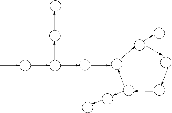
We will always assume that the lengths of all the tails of the one-loop automata are not bigger than the size of the $(1,1)$-loop. The following is an easy proposition and we omit its proof.

By Lemma 3.3, transforming a given automaton to an equivalent standard automaton may blow up the number of states exponentially. However, there is only polynomial blow up if $\mathcal{A}$ is a one-loop automaton.

Note that the equivalent standard automaton has $2p$ (1,1)-states. From each of them there is a $(1,\diamond)$-tail of length $p$ and a $(\diamond,1)$-tail of length $p$. Hence the automaton has $4p^{2}$ states. By the above lemma, we always assume the input automaton $\mathcal{A}$ is standard. In the rest of the paper, we will state all results in terms of the loop constant $p$ instead of $n$, the number of states of the input automaton. Since $p\leq n$, for any constant $c>0$, an $O(p^{c})$ algorithm can also be viewed as an $O(n^{c})$ algorithm.

Given two unary automatic graphs of finite degree $\mathcal{G}_{1}=(V,E_{1})$ and $\mathcal{G}_{2}=(V,E_{2})$ (where we recall the convention that the domain of each graph is $1^{\star}$), we can form the union graph $\mathcal{G}_{1}\oplus\mathcal{G}_{2}=(V,E_{1}\cup E_{2})$ and the intersection graph $\mathcal{G}_{1}\otimes\mathcal{G}_{2}=(V,E_{1}\cap E_{2})$. Automatic graphs of finite degree are closed under these operations. Indeed, let $\mathcal{A}_{1}$ and $\mathcal{A}_{2}$ be one-loop automata recognizing $E_{1}$ and $E_{2}$ with loop constants $p_{1}$ and $p_{2}$, respectively. The standard construction that builds automata for the union and intersection operations produces a one-loop automaton whose loop constant is $p_{1}\cdot p_{2}$. We introduce another operation: consider the new graph $\mathcal{G}_{1}^{\prime}=(V,E_{1}^{\prime})$, where the set $E_{1}^{\prime}$ of edges is defined as follows; a pair $(1^{n},1^{m})$ is in $E^{\prime}$ if and only if $(1^{n},1^{m})\notin E$ and $|n-m|\leq p_{1}$. The relation $E_{1}^{\prime}$ is recognized by the same automaton as $E_{1}$, modified so that all $(\diamond,1)$-states that are final declared non-final, and all the $(\diamond,1)$-states that are non-final declared final. Thus, we have the following proposition:

Now our goal is to recast Theorem 3.4 for graphs of finite degree. Our analysis will show that, in contrast to the general case for automatic graphs, the parameters $\mathcal{B}$, $\mathcal{D}$, and $\bar{R}$ for graphs of finite degree can be extracted in linear time.

Thus $\mathcal{G}_{\alpha}$ is obtained by taking $\mathcal{D}$ together with an infinite disjoint union of $\mathcal{F}$ such that edges between $\mathcal{D}$ and the first copy of $\mathcal{F}$ are put according to the mapping $\eta$, and edges between successive copies of $\mathcal{F}$ are put according to $\sigma_{i}$.

Figure 3 illustrates the general shape of a unary automatic graph of finite degree that is build from $\mathcal{D}$, $\mathcal{F}$, $\eta$, and $\sigma^{\omega}$, where $\sigma^{\omega}$ is the infinite word $\sigma\sigma\sigma\cdots$.

The proof of the above theorem also gives us the following corollary.

Recall the graphs are undirected. A component of $\mathcal{G}$ is the transitive closure of a vertex under the edge relation. The infinite component problem asks whether a given graph $\mathcal{G}$ has an infinite component.

By Theorem 4.5, let $\mathcal{G}=\mathcal{G}_{\eta\sigma^{\omega}}$. We observe that it is sufficient to consider the case in which $\mathcal{D}=\emptyset$ (hence $\mathcal{G}=\mathcal{G}_{\sigma^{\omega}}$) since $\mathcal{G}_{\eta\sigma^{\omega}}$ has an infinite component if and only if $\mathcal{G}_{\sigma^{\omega}}$ has one.

Let $\mathcal{F}^{i}$ be the $i^{th}$ copy of $\mathcal{F}$ in $\mathcal{G}$. Let $x^{i}$ be the copy of vertex $x$ in $\mathcal{F}^{i}$. We construct a finite directed graph $\mathcal{F}^{\sigma}=(V^{\sigma},E^{\sigma})$ as follows. Each node in $V^{\sigma}$ represents a distinct connected component in $\mathcal{F}$. For simplicity, we assume that $|V^{\sigma}|=|V_{\mathcal{F}}|$ and hence use $x$ to denote its own component in $\mathcal{F}$. The case in which $|V^{\sigma}|<|V_{\mathcal{F}}|$ can be treated in a similar way. For $x,y\in V_{\mathcal{F}}$, put $(x,y)\in E^{\sigma}$ if and only if $y^{\prime}\in\sigma(x^{\prime})$ for some $x^{\prime}$ and $y^{\prime}$ that are in the same component as $x$ and $y$, respectively. Constructing $\mathcal{F}^{\sigma}$ requires finding connected components of $\mathcal{F}$ hence takes time $O(p^{2})$. To prove the above theorem, we make essential use of the following definition. See also [HellNes04].

In an oriented walk $\mathcal{P}$, an arc $(v_{i},v_{i+1})$ is called a forward arc and $(v_{i+1},v_{i})$ is called a backward arc. The net length of $\mathcal{P}$, denoted $disp(\mathcal{P})$, is the difference between the number of forward arcs and backward arcs. Note the net length can be negative. The next lemma establishes a connection between oriented cycles in $\mathcal{F}^{\sigma}$ and infinite components in $\mathcal{G}$.

We next turn our attention to the infinity testing problem for unary automatic graphs of finite degree. Recall that this problem asks for an algorithm that, given a vertex $v$ and a graph $\mathcal{G}$, decides if $v$ belongs to an infinite component. We prove the following theorem.

For a fixed input $x^{i}$, we have the following lemma.

Let $i^{\prime}=min\{p,i\}$. To decide if $x^{i}$ and $y^{j}$ are in the same component, we run a breadth first search in $\mathcal{G}$ starting from $x^{i}$ and going through all vertices in $\mathcal{F}^{i-i^{\prime}},\ldots,\mathcal{F}^{i+p}$. The algorithm is as follows:

Note that any $y^{j}$ is reachable from $x^{i}$ on the graph $\mathcal{G}$ restricted on $\mathcal{F}^{i-i^{\prime}},\ldots,\mathcal{F}^{i+p}$ if and only if after running FiniteReach on the input $x^{i}$, the pair $(y,j-i)$ is in $Q$. When running the algorithm we only use the exact value of the input $i$ when $i<p$ (we set $i^{\prime}=p-1$ whenever $i\geq p$), so the running time of FiniteReach is bounded by the number of edges in $\mathcal{G}$ restricted to $\mathcal{F}^{0},\ldots,\mathcal{F}^{2p}$. Therefore the running time is $O(p^{3})$. Let $B=\{y\mid(y,p)\in Q\}$.

Suppose $\mathcal{G}$ is a unary automatic graph of finite degree represented by an automaton with loop constant $p$. The reachability problem on $\mathcal{G}$ is formulated as: given two vertices $x^{i},y^{j}$ in $\mathcal{G}$, decide if $x^{i}$ and $y^{j}$ are in the same component. We prove the following theorem.

We restrict to the case when $\mathcal{G}=\mathcal{G}_{\sigma^{\omega}}$. The proof can be modified slightly to work in the more general case, $\mathcal{G}=\mathcal{G}_{\eta\sigma^{\omega}}$.

Since, by Theorem 6.1, there is an $O(p^{3})$-time algorithm to check if $x^{i}$ is in a finite component, we can work on the two possible cases separately. We first deal with the case when the input $x^{i}$ is in a finite component. By Lemma 6.2, $x^{i}$ and $y^{j}$ are in the same (finite) component if and only if after running FiniteReach on the input $x^{i}$, the pair $(y,j-i)$ is in the queue $Q$.

Now, suppose that $x^{i}$ is in an infinite component. We start with the following question: given $y\in V_{\mathcal{F}}$, are $x^{i}$ and $y^{i}$ in the same component in $\mathcal{G}$? To answer this, we present an algorithm that computes all vertices $y\in V_{\mathcal{F}}$ whose $i^{th}$ copy lies in the same $\mathcal{G}$-component as $x^{i}$. The algorithm is similar to FiniteReach, except that it does not depend on the input $i$. Line(3b) in the algorithm is changed to the following:

We use this modified algorithm to define the set $Reach(x)=\{y\mid(y,0)\in Q\}$. Intuitively, we can think of the algorithm as a breadth first search through $\mathcal{F}^{0}\cup\cdots\cup\mathcal{F}^{2p}$ which originates at $x^{p}$. Therefore, $y\in Reach(x)$ if and only if there exists a path from $x^{p}$ to $y^{p}$ in $\mathcal{G}$ restricted to $\mathcal{F}^{0}\cup\cdots\cup\mathcal{F}^{2p}$.

References

- [Blu99] A. Blumensath, Automatic Structures. Diploma Thesis, RWTH Aachen, 1999.
- [BluGr04] A. Blumensath, E. Grädel, Finite presentations of infinite structures: Automata and interpretations. Theory of Computing Systems, vol. 37, pp. 642-674, 2004.
- [BouEspMal97] A. Bouajjani, J. Esparza, and O. Maler. Reachability analysis of pushdown automata: Application to model-checking. In Proceedings of CONCUR’97, LNCS 1243, pages 135-150, 1997.
- [Buc60] J. R. Büchi, On a decision method in restricted second-order arithmetic. Proc. International Congress on Logic, Methodology and Philosophy of Science (E. Nagel, P. Suppes, A. Tarski, Eds.), Stanford University Press, 1-11, 1960.
- [Cau02] D. Caucal, On infinite graphs having a decidable monadic theory. In Proc. 27th MFCS (K. Diks, W. Rytter, Eds.), Springer LNCS 2420, 165-176, 2002.
- [EHRS00] J. Esparza, D. Hansel, P. Rossmanith, S. Schwoon, Efficient algorithms for model checking pushdown systems, Proc. CAV 2000, LNCS 1855, Springer-Verlag, 232-247, 2000.
- [HellNes04] P. Hell, J. Nešetřil, Graphs and Homomorphisms. Oxford University Press, 2004.
- [Hodg76] B. R. Hodgson, Théories décidables par automate fini.. Phd thesis, University of Montréal, 1976.
- [KhoMin] B. Khoussainov, M. Minnes, Automatic structures and their complexity.(Extended Abstract). Proc. TAMC, to appear, 2008.
- [KhoNer95] B. Khoussainov, A. Nerode, Automatic presentation of structures. Lecture Notes in Computer Science, 960; 367-392, 1995.
- [KNRS04] B. Khoussainov, A. Nies, S. Rubin, F. Stephan, Automatic structures: richness and limitations. In Proc. 19th LICS: 44-53, 2004.
- [KhoRub01] B. Khoussainov, S. Rubin, Graphs with automatic presentations over a unary alphabet. Journal of Automata, Languages and Combinatorics 6(4): 467-480, 2001.
- [KhRS05] B. Khoussainov, S. Rubin, F. Stephan, Automatic linear orders and trees. ACM Trans. Comput. Log. 6(4): 675-700, 2005.
- [Lib04] L. Libkin, Elements of finite model theory. Springer-Verlag, 2004.
- [Loh03] M. Lohrey, Automatic structures of bounded degree. In Proc. 10th International Conference on Logic for Programming, Artificial Intelligence, and Reasoning (LPAR), LNAI 2850: 344 - 358, 2003.
- [OliTho05] G. P. Oliver, R. M. Thomas, Automatic presentations for finitely generated groups. in Proc. 22nd STACS (V. Diekert, B.Durand, Eds.), Springer, LNCS 3404: 693 - 704, 2005.
- [Rab69] M.O. Rabin, Decidability of second-order theories and automata on infinite trees, Trans. Amer. Math. Soc. 141, 1-35, 1969.
- [Rub04] S. Rubin, Automatic Structures, PhD Thesis, University of Auckland, 2004.
- [Tho02] W. Thomas, A short introduction to infinite automata, In Proceedings of the 5th International Conference Development in Language Theory, Springer, LNCS 2295: 130-144, 2002.
- [WohTho04] S. Wöhrle, W. Thomas, Model Checking Synchronized Products of Infinite Transition Systems, In Proc. 19th Annual IEEE Symposium on Logic in Computer Science (LICS’04), pp. 2-11, 2004.