跳到论文正文
W Papers独立论文阅读器 arXiv:0809.3328 论文正文 计算阅读时间 · 0%
引用这篇论文根据当前论文元数据生成,正式投稿前建议核对。


License: arXiv.org perpetual non-exclusive license
arXiv:0809.3328v1 [cond-mat.stat-mech] 19 Sep 2008

Nonlinear response and fluctuation dissipation relations

Eugenio Lippiello† Affiliation: Dipartimento di Scienze Fisiche, Universitá di Napoli “Federico II”, 80125 Napoli, Italy.    Federico Corberi‡, Alessandro Sarracino and Marco Zannetti§ Affiliation: Dipartimento di Matematica ed Informatica via Ponte don Melillo, Università di Salerno, 84084 Fisciano (SA), Italy
Abstract

A unified derivation of the off equilibrium fluctuation dissipation relations (FDR) is given for Ising and continous spins to arbitrary order, within the framework of Markovian stochastic dynamics. Knowledge of the FDR allows to develop zero field algorithms for the efficient numerical computation of the response functions. Two applications are presented. In the first one, the problem of probing for the existence of a growing cooperative length scale is considered in those cases, like in glassy systems, where the linear FDR is of no use. The effectiveness of an appropriate second order FDR is illustrated in the test case of the Edwards-Anderson spin glass in one and two dimensions. In the second one, the important problem of the definition of an off equilibrium effective temperature through the nonlinear FDR is considered. It is shown that, in the case of coarsening systems, the effective temperature derived from the second order FDR is consistent with the one obtained from the linear FDR.

†lippiello@sa.infn.it ‡corberi@sa.infn.it ¶sarracino@sa.infn.it §zannetti@sa.infn.it

PACS: 05.70.Ln, 75.40.Gb, 05.40.-a

I Introduction

The statistical mechanics of systems out of equilibrium is a rapidly evolving subject, due to the intensive research in the slow relaxation phenomena arising in several different contexts, such as coarsening systems, glassy and granular materials, colloidal systems etc. Understanding the basic mechanism underlying the slow relaxation is an issue of major importance. In particular, a key question is whether the large time scales are due to cooperative effects on large length scales. For non disordered coarsening systems this is certainly the case, since the observed power law relaxation can be directly related to the growth of the time dependent correlation length, or domain size [1]. In the case of disordered or glassy systems the establishment of such a connection is much more problematic, due to the difficulty of pinpointing the observables fit to the task.

The use of the nonlinear susceptibilities has been advocated  [2, 3, 4] as experimental or numerical probe apt to detect the heterogeneous character of the glassy relaxation and, possibly, to uncover the existence of the growing length scale responsible of the slowing down of the relaxation. However, this requires to establish clearly the relationship between non linear susceptibilities and correlation functions, in order to make sure what actually do the nonlinear susceptibilities probe. In other words, the problem of the derivation of the nonlinear fluctuation dissipation relations (FDR) in the out of equilibrium regime needs to be addressed. As a matter of fact, this has been one of the most fruitful lines of investigation in the field of slow relaxation, although mostly limited to the domain of linear response [5, 6].

In this paper we approach the problem on fairly general grounds. Within the framework of Markovian stochastic evolution, we bring to the fore the structural elements which are common to discrete and continous spins. We develop the formal apparatus necessary for a unified derivation of the FDR in the two cases and to arbitrary order. We also show, expanding on the work of Semerjian et al. [7], how the nonlinear FDR of arbitrary order can be derived from a fluctuation principle [8] also in the off equilibrium regime. This allows to regard the FDR as a manifestation of the constraint imposed on the dynamics by the requirement of microscopic reversibility.

The immediate application of the FDR is in the development of algorithms for the computation of the response functions without the imposistion of an external perturbation, the so called zero field algorithms. The numerical advantages of a zero field algorithm are remarkable. These have been illustrated and discussed in detail, in the linear case, in a recent paper [9]. In the present paper we apply the zero field algorithm to the computation of the nonlinear response functions. We consider two cases, where knowledge of a nonlinear response function is required. The first one arises in the search for a growing length scale in the context of glassy systems, as mentioned above. The presence of quenched or self-induced disorder makes the linear response function short ranged, compelling to resort to the nonlinear ones. The second one deals with the extension of the effective temperature concept [10] to nonlinear order. This is an important and difficult problem. Here, we consider it in the context of non disordered coarsening systems, showing the consistency of the effective temperatures derived from the linear and the second order FDR.

The paper is organised as follows: the formal developments concerning the time evolution, the response functions, the FDR and the fluctuation principle are presented in sections 2, 3, 4 and 5, respectively. In section 6 the problem of the detection of a cooperative length trough a nonlinear susceptibility is addressed, while the effective temperature to nonlinear order is treated in section 7. Concluding remarks are presented in section 8.

II Formalism and time evolution

Let us consider a system in contact with a thermal reservoir, whose microscopic states are the configurations σ=[σi]\sigma=[\sigma_{i}] of the NN degrees of freedom, discrete or continous, placed on the discrete set of sites i=1,..,Ni=1,..,N. Assuming a Markovian stochastic dynamics, the time evolution of the system is fully specified once the probability distribution P⁡(σ,t0)P(\sigma,t_{0}) at some initial time t0t_{0} is given, together with the transition probability P(σ,t|σ′,t′)P(\sigma,t|\sigma^{\prime},t^{\prime}) for any pair of times t0≤t′≤tt_{0}\leq t^{\prime}\leq t. Observables, or random variables, are functions A⁡(σ)A(\sigma) defined over the phase space of the microscopic states, whose expectations are given by

⟨A⁡(t)⟩=∑σA⁡(σ)​P​(σ,t)\langle A(t)\rangle=\sum_{\sigma}A(\sigma)P(\sigma,t) (1)

where P(σ,t)=∑σ′P(σ,t|σ′,t0)P(σ′,t0)P(\sigma,t)=\sum_{\sigma^{\prime}}P(\sigma,t|\sigma^{\prime},t_{0})P(\sigma^{\prime},t_{0}).

In order to keep the notation compact, it is convenient to switch to the operator formalism [11], whereby the microscopic states introduced above are the set of labels of the basis vectors

|σ⟩=⨂|σi⟩,i=1,…N|\sigma\rangle=\bigotimes|\sigma_{i}\rangle,\;\;\;i=1,...N (2)

of a vector space. The single site states obey the orthonormality relation ⟨σi|σj′⟩=δσi,σj′​δi,j\langle\sigma_{i}|\sigma^{\prime}_{j}\rangle=\delta_{\sigma_{i},\sigma^{\prime}_{j}}\delta_{i,j}. With this notation, the probability distributions P⁡(σ,t)P(\sigma,t) become the time dependent vectors |P⁡(t)⟩|P(t)\rangle such that

P⁡(σ,t)=⟨σ|P⁡(t)⟩P(\sigma,t)=\langle\sigma|P(t)\rangle (3)

and the transition probability is associated to the propagator of the process P^​(t|t′)\hat{P}(t|t^{\prime}), which is the operator whose matrix elements are given by

P(σ,t|σ′,t′)=⟨σ|P^(t|t′)|σ′⟩.P(\sigma,t|\sigma^{\prime},t^{\prime})=\langle\sigma|\hat{P}(t|t^{\prime})|\sigma^{\prime}\rangle. (4)

For stochastically continous processes, through the first order expansion

P^​(t+Δ​t|t)=I^+W^​(t)​Δ​t+𝒪⁡(Δ​t2)\hat{P}(t+\Delta t|t)=\hat{I}+\hat{W}(t)\Delta t+{\cal O}(\Delta t^{2}) (5)

where I^\hat{I} is the identity operator, there remains defined the generator of the process W^​(t)\hat{W}(t). Then, the pair |P​(t0)⟩,W^​(t)|P(t_{0})\rangle,\hat{W}(t) contains all the information on the process, since the propagator can be written as

P^​(t|t′)=𝒯⁡(e∫t′td​s​W^​(s))\hat{P}(t|t^{\prime})={\cal T}\left(e^{\int_{t^{\prime}}^{t}ds\hat{W}(s)}\right) (6)

where 𝒯{\cal T} is the time ordering operator. In differential form this is equivalent to the equations

∂∂t​P^​(t|t′)=W^​(t)​P^​(t|t′){\partial\over\partial t}\hat{P}(t|t^{\prime})=\hat{W}(t)\hat{P}(t|t^{\prime}) (7)
∂∂t′​P^​(t|t′)=−P^​(t|t′)​W^​(t′){\partial\over\partial t^{\prime}}\hat{P}(t|t^{\prime})=-\hat{P}(t|t^{\prime})\hat{W}(t^{\prime}) (8)

from the first one of which follows the equation of motion of the state vector

∂∂t​|P⁡(t)⟩=W^​(t)​|P⁡(t)⟩.{\partial\over\partial t}|P(t)\rangle=\hat{W}(t)|P(t)\rangle. (9)

Notice that the normalization of probabilities imposes on the generator the condition

⟨−|W^(t)=0\langle-|\hat{W}(t)=0 (10)

where ⟨−|=∑σ⟨σ|\langle-|=\sum_{\sigma}\langle\sigma| is called the flat vector. We shall assume that at each instant of time the generator satisfies the detailed balance condition

eβ​ℋ^​(t)​W^​(t)​e−β​ℋ^​(t)=W^†​(t)e^{\beta\hat{{\cal H}}(t)}\hat{W}(t)e^{-\beta\hat{{\cal H}}(t)}=\hat{W}^{\dagger}(t) (11)

where ℋ^​(t)\hat{{\cal H}}(t) denotes the Hamiltonian of the system, with a possible time dependence. This implies that the istantaneous Gibbs state

|P⁡(t)⟩β=1Z⁡(t)​e−β​ℋ^​(t)​|−⟩|P(t)\rangle_{\beta}={1\over Z(t)}e^{-\beta\hat{{\cal H}}(t)}|-\rangle (12)

is an invariant state in the sense that

W^​(t)​|P⁡(t)⟩β=0.\hat{W}(t)|P(t)\rangle_{\beta}=0. (13)

The time dependent partition function is given by Z⁡(t)=⟨−|e−β​ℋ^​(t)|−⟩Z(t)=\langle-|e^{-\beta\hat{{\cal H}}(t)}|-\rangle, as it follows from the normalization of the state ⟨−|P(t)⟩β=1\langle-|P(t)\rangle_{\beta}=1. From now on we shall adopt the notation |⋅⟩β|\cdot\rangle_{\beta} for the Gibbs states.

Notice that Eq. (1) requires that observables correspond to diagonal operators. Each random function A⁡(σ)A(\sigma) is mapped into the operator A^=A⁡(σ^)\hat{A}=A(\hat{\sigma}), where the operators σ^i\hat{\sigma}_{i} are defined by

σ^i​|σ⟩=σi​|σ⟩\hat{\sigma}_{i}|\sigma\rangle=\sigma_{i}|\sigma\rangle (14)

in such a way that the expectation (1) can be written as

⟨A^​(t)⟩=⟨−|A^|​P​(t)⟩.\langle\hat{A}(t)\rangle=\langle-|\hat{A}|P(t)\rangle. (15)

If W^\hat{W} and |P⟩β|P\rangle_{\beta} are time independent, one can show that the multi-time expectations of observables in the stationary state obey the Onsager relation [12]. Namely, if A^1,A^2,…,A^n\hat{A}_{1},\hat{A}_{2},...,\hat{A}_{n} is a set of observables and tn≥tn−1​…≥t1t_{n}\geq t_{n-1}...\geq t_{1} an ordered sequence of instants of time, then

⟨A^n​(tn)​A^n−1​(tn−1)​…​A^2​(t2)​A^1​(t1)⟩β=\displaystyle\langle\hat{A}_{n}(t_{n})\hat{A}_{n-1}(t_{n-1})...\hat{A}_{2}(t_{2})\hat{A}_{1}(t_{1})\rangle_{\beta}=
⟨A^1​(tn)​A^2​(tn−(t2−t1))​…​A^n−1​(t1+(tn−tn−1))​A^n​(t1)⟩β\displaystyle\langle\hat{A}_{1}(t_{n})\hat{A}_{2}(t_{n}-(t_{2}-t_{1}))...\hat{A}_{n-1}(t_{1}+(t_{n}-t_{n-1}))\hat{A}_{n}(t_{1})\rangle_{\beta} (16)

where

⟨A^n​(tn)​A^n−1​(tn−1)​…​A^2​(t2)​A^1​(t1)⟩β=\displaystyle\langle\hat{A}_{n}(t_{n})\hat{A}_{n-1}(t_{n-1})...\hat{A}_{2}(t_{2})\hat{A}_{1}(t_{1})\rangle_{\beta}=
⟨−|A^n​P^​(tn|tn−1)​A^n−1​…​A^2​P^​(t2|t1)​A^1|​P⟩β.\displaystyle\langle-|\hat{A}_{n}\hat{P}(t_{n}|t_{n-1})\hat{A}_{n-1}...\hat{A}_{2}\hat{P}(t_{2}|t_{1})\hat{A}_{1}|P\rangle_{\beta}. (17)

Finally, using Eqs. (7) and (8), it is straightforward to show that the time derivative of a multi-time expectation is given by

∂∂tk⟨A^n(tn)..A^k(tk)..A^1(t1)⟩=\displaystyle{\partial\over\partial t_{k}}\langle\hat{A}_{n}(t_{n})..\hat{A}_{k}(t_{k})..\hat{A}_{1}(t_{1})\rangle=
⟨A^n(tn)..[A^k,W^(tk)](tk)..A^1(t1)⟩\displaystyle\langle\hat{A}_{n}(t_{n})..[\hat{A}_{k},\hat{W}(t_{k})](t_{k})..\hat{A}_{1}(t_{1})\rangle (18)

namely, the time derivative in front of the expectation amounts to the insertion, at the time tkt_{k}, of the commutator [A^k,W^​(tk)][\hat{A}_{k},\hat{W}(t_{k})] inside the expectation. This applies for all k=1,..,nk=1,..,n. In particular, in the case of a single observable

∂∂t​⟨A^​(t)⟩=⟨−|A^​W^​(t)|​P​(t)⟩=⟨−|[A^,W^​(t)]|​P​(t)⟩{\partial\over\partial t}\langle\hat{A}(t)\rangle=\langle-|\hat{A}\hat{W}(t)|P(t)\rangle=\langle-|[\hat{A},\hat{W}(t)]|P(t)\rangle (19)

where the second equality is a consequence of Eq. (10). It should be noticed that, in general, [A^,W^​(t)][\hat{A},\hat{W}(t)] is not an observable.

III Response functions

Let us assume that the generator W^​(t)\hat{W}(t) depends on time through an external field hi​(t)h_{i}(t). Then, upon varying hi​(t)h_{i}(t), there remains defined a family of stochastic processes and one may ask whether these stochastic processes are related one to the other. In particular, one would like to know whether the process with the generic hi​(t)h_{i}(t) can be reconstructed from the properties of the unperturbed process, the one with the particular choice hi​(t)≡0h_{i}(t)\equiv 0. In order to answer the question, let us start from the statement that all the information in the process, with a given hi​(t)h_{i}(t), is contained in the full hierarchy of the time dependent moments

Mi1,…,in​(t1,…,tn,[hi​(t′)])=⟨σ^i1​(t1)​…​σ^in​(tn)⟩M_{i_{1},...,i_{n}}(t_{1},...,t_{n},[h_{i}(t^{\prime})])=\langle\hat{\sigma}_{i_{1}}(t_{1})...\hat{\sigma}_{i_{n}}(t_{n})\rangle (20)

each of which is a functional of hi​(t)h_{i}(t). Assuming analiticity, one can write the formal expansion

Mi1..in(t1,..,tn,[hi(t′)])=Mi1..in(t1,..,tn)+\displaystyle M_{i_{1}..i_{n}}(t_{1},..,t_{n},[h_{i}(t^{\prime})])=M_{i_{1}..i_{n}}(t_{1},..,t_{n})+ (21)
∑m=1∞1m!∑j1..jm∫twtdt1′…∫twtdtm′Ri1..in;j1..jm(n,m)(t1,..,tn;t1′,..,tm′)hj1(t1′)…hjm(tm′)\displaystyle\sum_{m=1}^{\infty}{1\over m!}\sum_{j_{1}..j_{m}}\int_{t_{w}}^{t}dt^{\prime}_{1}...\int_{t_{w}}^{t}dt^{\prime}_{m}\;R^{(n,m)}_{i_{1}..i_{n};j_{1}..j_{m}}(t_{1},..,t_{n};t^{\prime}_{1},..,t^{\prime}_{m})h_{j_{1}}(t^{\prime}_{1})...h_{j_{m}}(t^{\prime}_{m})

where Mi1..in(t1,..,tn)M_{i_{1}..i_{n}}(t_{1},..,t_{n}) is the unperturbed moment, (tw,t)(t_{w},t) is the time interval over which the action of the external field is considered, and

Ri1..in;j1..jm(n,m)(t1,..,tn;t1′,..,tm′)=δmMi1..in(t1,..,tn,[hi(t′)])δ​hj1​(t1′)​…​δ​hjm​(tm′)|h=0R^{(n,m)}_{i_{1}..i_{n};j_{1}..j_{m}}(t_{1},..,t_{n};t^{\prime}_{1},..,t^{\prime}_{m})=\left.{\delta^{m}M_{i_{1}..i_{n}}(t_{1},..,t_{n},[h_{i}(t^{\prime})])\over\delta h_{j_{1}}(t^{\prime}_{1})...\delta h_{j_{m}}(t^{\prime}_{m})}\right|_{h=0} (22)

is the mm-th order response function of the nn-th moment. Therefore, the question asked above can be positively answered if the response functions can be expressed in terms of quantities computable in the unperturbed process, namely if the FDR of arbitrary order can be obtained.

Without loss of generality, we limit ourselves to work out the response functions for the first moment. For the responses of the higher moments there is nothing conceptually different, just the formalism gets more involved. As a matter of fact, in section VI we shall deal with the second order response of the second moment. Coming back to the first moment, from

Mi​(t,[hj​(t′)])=⟨−|σ^i​P^h​(t|tw)|​P​(tw)⟩M_{i}(t,[h_{j}(t^{\prime})])=\langle-|\hat{\sigma}_{i}\hat{P}_{h}(t|t_{w})|P(t_{w})\rangle (23)

where P^h​(t|tw)\hat{P}_{h}(t|t_{w}) is the propagator in the presence of the field, follows

Ri;j1..jm(1,m)(t,t1,..,tm)=⟨−|σ^iδm​P^h​(t|tw)δ​hj1​(t1)​…​δ​hjm​(tm)|h=0|P(tw)⟩R^{(1,m)}_{i;j_{1}..j_{m}}(t,t_{1},..,t_{m})=\langle-|\hat{\sigma}_{i}\left.{\delta^{m}\hat{P}_{h}(t|t_{w})\over\delta h_{j_{1}}(t_{1})...\delta h_{j_{m}}(t_{m})}\right|_{h=0}|P(t_{w})\rangle (24)

which obviously vanishes if tj∉(tw,t)t_{j}\not\in(t_{w},t) for any j=1,..,mj=1,..,m. Let us write explicitely the first two derivatives

δ​P^h​(t|tw)δ​hj1​(t1)\displaystyle{\delta\hat{P}_{h}(t|t_{w})\over\delta h_{j_{1}}(t_{1})} =\displaystyle= 𝒯⁡[e∫twtd​s​W^​(s)​∂W^​(t1)∂hj1​(t1)]\displaystyle{\cal T}\left[e^{\int_{t_{w}}^{t}ds\hat{W}(s)}{\partial\hat{W}(t_{1})\over\partial h_{j_{1}}(t_{1})}\right] (25)
=\displaystyle= P^h​(t|t1)​∂W^​(t1)∂hj1​(t1)​P^h​(t1|tw)\displaystyle\hat{P}_{h}(t|t_{1}){\partial\hat{W}(t_{1})\over\partial h_{j_{1}}(t_{1})}\hat{P}_{h}(t_{1}|t_{w})

and

δ2​P^h​(t|tw)δ​hj1​(t1)​δ​hj2​(t2)\displaystyle{\delta^{2}\hat{P}_{h}(t|t_{w})\over\delta h_{j_{1}}(t_{1})\delta h_{j_{2}}(t_{2})} =\displaystyle= 𝒯⁡{e∫twtd​s​W^​(s)​[∂W^​(t1)∂hj1​(t1)​∂W^​(t2)∂hj2​(t2)+∂2W^​(t1)∂hj12​(t1)​δ​(12)]}\displaystyle{\cal T}\left\{e^{\int_{t_{w}}^{t}ds\hat{W}(s)}\left[{\partial\hat{W}(t_{1})\over\partial h_{j_{1}}(t_{1})}{\partial\hat{W}(t_{2})\over\partial h_{j_{2}}(t_{2})}+{\partial^{2}\hat{W}(t_{1})\over\partial h_{j_{1}}^{2}(t_{1})}\delta(12)\right]\right\} (26)
=\displaystyle= P^h​(t|tM)​∂W^​(tM)∂hjM​(tM)​P^h​(tM|tm)​∂W^​(tm)∂hjm​(tm)​P^h​(tm|tw)\displaystyle\hat{P}_{h}(t|t_{M}){\partial\hat{W}(t_{M})\over\partial h_{j_{M}}(t_{M})}\hat{P}_{h}(t_{M}|t_{m}){\partial\hat{W}(t_{m})\over\partial h_{j_{m}}(t_{m})}\hat{P}_{h}(t_{m}|t_{w})
+\displaystyle+ P^h​(t|t1)​∂2W^​(t1)∂hj12​(t1)​P^h​(t1|tw)​δ​(12)\displaystyle\hat{P}_{h}(t|t_{1}){\partial^{2}\hat{W}(t_{1})\over\partial h_{j_{1}}^{2}(t_{1})}\hat{P}_{h}(t_{1}|t_{w})\delta(12)

where tM=max⁡(tj)t_{M}=\max(t_{j}), tm=min⁡(tj)t_{m}=\min(t_{j}), jM,jmj_{M},j_{m} are the sites where the field acts at the times tMt_{M} or tmt_{m}, respectively, and δ⁡(n​p)=δjn,jp​δ​(tn−tp)\delta(np)=\delta_{j_{n},j_{p}}\delta(t_{n}-t_{p}). The third order derivative is written down in Appendix I.

In order to go further, we must specify how W^​(t)\hat{W}(t) depends on the field hi​(t)h_{i}(t) and that is where the distinction between discrete spins and continous spins comes in. In the following, in order to keep the derivation as simple as possible we shall specialize to the case of Ising spins with single spin-flip dynamics. The generalization to qq-state spins (e.g. clock models) and to dinamical rules with conservation laws, such as Kawasaki spin-exchange, turns out to be straightforward.

III.1 Ising spins

For Ising spins the state vectors |σi=±1⟩|\sigma_{i}=\pm 1\rangle are represented by the column vectors

|σi=1⟩=(10),|σi=−1⟩=(01).|\sigma_{i}=1\rangle=\left(\begin{array}[]{c}1\\ 0\\ \end{array}\right),\;\;\;\;|\sigma_{i}=-1\rangle=\left(\begin{array}[]{c}0\\ 1\\ \end{array}\right).

A generator of single spin flip dynamics is of the type

W^=1N​∑i=1NW^i\hat{W}={1\over N}\sum_{i=1}^{N}\hat{W}_{i} (27)

where W^i\hat{W}_{i} has non vanishing matrix elements only between states which differ for the value of σi\sigma_{i}. The form of W^i\hat{W}_{i} is obtained imposing the detailed balance condition (11). Singling out the site ii, the Hamiltonian can be written in the form

ℋ^​(t)=ℋ⁡([σ^z]i,t)+{hW​([σ^z]i)−hi​(t)}​σ^iz,\hat{{\cal H}}(t)={\cal H}([\hat{\sigma}^{z}]_{i},t)+\{h^{W}([\hat{\sigma}^{z}]_{i})-h_{i}(t)\}\hat{\sigma}^{z}_{i}, (28)

where σ^iz\hat{\sigma}^{z}_{i} is the zz Pauli matrix

σ^iz=(100−1),\hat{\sigma}^{z}_{i}=\left(\begin{array}[]{cc}1&0\\ 0&-1\\ \end{array}\right),

[σ^z]i[\hat{\sigma}^{z}]_{i} stands for the set of all spins except for the one on the ii-th site and h^iW=hW​([σ^z]i)\hat{h}^{W}_{i}=h^{W}([\hat{\sigma}^{z}]_{i}) is the Weiss field on the site ii. Inserting into the detailed balance condition (11), one finds the generator of the Glauber type [13]

W^i​(t)=(σ^ix−I^)​eβ⁡[h^iW−hi​(t)]​σ^iz\hat{W}_{i}(t)=(\hat{\sigma}^{x}_{i}-\hat{I})e^{\beta[\hat{h}^{W}_{i}-h_{i}(t)]\hat{\sigma}^{z}_{i}} (29)

where σ^ix\hat{\sigma}^{x}_{i} is the xx Pauli matrix

σ^ix=(0110).\hat{\sigma}^{x}_{i}=\left(\begin{array}[]{cc}0&1\\ 1&0\\ \end{array}\right).

Hence, the derivatives are given by

∂nW^​(t1)∂hj1n​(t1)=(−β)n​W^j1​(t1)​(σ^j1z)n{\partial^{n}\hat{W}(t_{1})\over\partial h_{j_{1}}^{n}(t_{1})}=(-\beta)^{n}\hat{W}_{j_{1}}(t_{1})(\hat{\sigma}^{z}_{j_{1}})^{n} (30)

with

(σ^j1z)n={I^,for​n​evenσ^j1z,for​n​odd.(\hat{\sigma}^{z}_{j_{1}})^{n}=\left\{\begin{array}[]{ll}\hat{I},\;\;$for$\;\;n\;\;$even$\\ \hat{\sigma}^{z}_{j_{1}},\;\;$for$\;\;n\;\;$odd$.\end{array}\right. (31)

For later reference, let us write here the identity

W^i​σ^iz=12​[W^i,σ^iz]+12​{W^i,σ^iz}\hat{W}_{i}\hat{\sigma}^{z}_{i}={1\over 2}[\hat{W}_{i},\hat{\sigma}^{z}_{i}]+{1\over 2}\{\hat{W}_{i},\hat{\sigma}^{z}_{i}\} (32)

obtained by adding the commutator and the anticommutator. It is straightforward to verify that the anticommutator is a diagonal operator and, therefore, is an observable which we will denote by

B^i​(t)={σ^iz,W^​(t)}.\hat{B}_{i}(t)=\{\hat{\sigma}^{z}_{i},\hat{W}(t)\}. (33)

Due to Eq. (10), the average of the left hand side of Eq. (32) vanishes and Eq. (19) for σ^iz\hat{\sigma}^{z}_{i} can be rewritten as

∂∂t​⟨σ^iz​(t)⟩=⟨B^i​(t)⟩.{\partial\over\partial t}\langle\hat{\sigma}^{z}_{i}(t)\rangle=\langle\hat{B}_{i}(t)\rangle. (34)

III.2 Continuous spins

In order to avoid confusion, here we shall denote by φ=[φi]\varphi=[\varphi_{i}] the set of the NN continuous variables. Let us assume an equation of motion of the Langevin type

∂∂t​φi​(t)=Bi​(t)+ηi​(t){\partial\over\partial t}\varphi_{i}(t)=B_{i}(t)+\eta_{i}(t) (35)

where the drift BiB_{i} is related to the Hamiltonian, or free energy functional ℋ⁡[φ]{\cal H}[\varphi], by

Bi​(t)=−∂ℋ⁡[φ⁡(t)]∂φiB_{i}(t)=-{\partial{\cal H}[\varphi(t)]\over\partial\varphi_{i}} (36)

ηi​(t)\eta_{i}(t) is a gaussian white noise with expectations

⟨ηi​(t)⟩=0,⟨ηi​(t)​ηj​(t′)⟩=2​T​δi,j​δ​(t−t′)\langle\eta_{i}(t)\rangle=0,\;\;\;\;\;\langle\eta_{i}(t)\eta_{j}(t^{\prime})\rangle=2T\delta_{i,j}\delta(t-t^{\prime}) (37)

and TT is the temperature of the thermal reservoir. The generator of the corresponding Markov process is the Fokker-Planck operator

W^F​P=∑iW^iF​P\hat{W}^{FP}=\sum_{i}\hat{W}_{i}^{FP} (38)

where

W^iF​P=−{T​p^i2+i​Bi​[φ^]​p^i+Di​[φ^]},\hat{W}_{i}^{FP}=-\{T\hat{p}_{i}^{2}+iB_{i}[\hat{\varphi}]\hat{p}_{i}+D_{i}[\hat{\varphi}]\}, (39)

Bi​[φ^]B_{i}[\hat{\varphi}] is defined through Eq. (36) and

Di​[φ^]=−∂2ℋ⁡[φ]∂φi2|φ=φ^.D_{i}[\hat{\varphi}]=-\left.{\partial^{2}{\cal H}[\varphi]\over\partial\varphi_{i}^{2}}\right|_{\varphi=\hat{\varphi}}. (40)

The conjugated operators φ^i\hat{\varphi}_{i} and p^i\hat{p}_{i}, defined by

⟨φ′|φ^i|φ⟩=φi​⟨φ′|φ⟩\langle\varphi^{\prime}|\hat{\varphi}_{i}|\varphi\rangle=\varphi_{i}\langle\varphi^{\prime}|\varphi\rangle (41)
⟨φ′|p^i|φ⟩=−i​∂∂φi​⟨φ′|φ⟩\langle\varphi^{\prime}|\hat{p}_{i}|\varphi\rangle=-i{\partial\over\partial\varphi_{i}}\langle\varphi^{\prime}|\varphi\rangle (42)

obey the commutation relation

[φ^i,p^j]=i​δi,j[\hat{\varphi}_{i},\hat{p}_{j}]=i\delta_{i,j} (43)

and satisfy the equalities

⟨−|p^i=0\langle-|\hat{p}_{i}=0 (44)
⟨−|W^iF​P=0.\langle-|\hat{W}_{i}^{FP}=0. (45)

The external field enters the free energy functional linearly

ℋh​[φ,t]=ℋ⁡[φ]−∑ihi​(t)​φi{\cal H}_{h}[\varphi,t]={\cal H}[\varphi]-\sum_{i}h_{i}(t)\varphi_{i} (46)

yielding

Bh,i​[φ,t]=Bi​[φ]+hi​(t),B_{h,i}[\varphi,t]=B_{i}[\varphi]+h_{i}(t), (47)

while Di​[φ]D_{i}[\varphi] remains unaltered. Therefore, the generator is changed into

W^h,iF​P=W^iF​P−i​hi​(t)​p^i\hat{W}_{h,i}^{FP}=\hat{W}_{i}^{FP}-ih_{i}(t)\hat{p}_{i} (48)

and the derivatives are given by

∂nW^h,iF​P∂hin​(t)={−i​p^i,for​n=10,for​n>1.{\partial^{n}\hat{W}_{h,i}^{FP}\over\partial h^{n}_{i}(t)}=\left\{\begin{array}[]{ll}-i\hat{p}_{i},\;\;$for$\;\;n=1\\ 0,\;\;$for$\;\;n>1.\end{array}\right. (49)

Obviously, the identity (32) holds also in this case

W^iF​P​φ^i=12​[W^iF​P,φ^i]+12​{W^iF​P,φ^i}\hat{W}_{i}^{FP}\hat{\varphi}_{i}={1\over 2}[\hat{W}_{i}^{FP},\hat{\varphi}_{i}]+{1\over 2}\{\hat{W}_{i}^{FP},\hat{\varphi}_{i}\} (50)

and, using the definiton (39) together with the commutation relation (43), it is not difficul to rewrite it in the more convenient form

i​p^i=β2​{[W^iF​P,φ^i]+Bi​[φ^]}.i\hat{p}_{i}={\beta\over 2}\left\{[\hat{W}_{i}^{FP},\hat{\varphi}_{i}]+B_{i}[\hat{\varphi}]\right\}. (51)

Again, since the average of the left hand side vanishes, we get the analogous of Eq. (34)

∂∂t​⟨φ^i​(t)⟩=⟨Bi​[φ^]​(t)⟩{\partial\over\partial t}\langle\hat{\varphi}_{i}(t)\rangle=\langle B_{i}[\hat{\varphi}](t)\rangle (52)

showing that the anticommutator (33) for Ising spins and the drift (36) for continous spins play the same role in the evolution, thus justifying the choice of the same notation.

IV Fluctuation dissipation relations

Let us now return to the general treatment, valid for discrete and continous spins alike, with the operator σ^\hat{\sigma} standing either for σ^z\hat{\sigma}^{z} or for φ^\hat{\varphi}, depending on the context. Which is the case, will be specified whenever necessary.

Comparing the left hand sides of Eqs. (32)and (51) with the first derivatives (30) and (49), we can write the basic equation in this paper

∂W^∂hi=−β2([W^i,σ^i)]+Bi[σ^]){\partial\hat{W}\over\partial h_{i}}={-\beta\over 2}\left([\hat{W}_{i},\hat{\sigma}_{i})]+B_{i}[\hat{\sigma}]\right) (53)

where, in the case of continous spins, the superscript FP on the Fokker-Planck operator has been dropped and, as specified above, B^i\hat{B}_{i} stands for

B^i={{σ^i,W^i},for Ising spinsBi​[φ^],for continous spins.\hat{B}_{i}=\left\{\begin{array}[]{ll}\{\hat{\sigma}_{i},\hat{W}_{i}\},\;\;$for Ising spins$\\ B_{i}[\hat{\varphi}],\;\;$for continous spins$.\end{array}\right. (54)

We are now in the position to derive the FDR, by going through the following steps:

  1. 1.

    according to Eq. (24), the response function is obtained by appropriate insertions of derivatives of the generator in between propagators, as exemplified in Eqs. (25) and (26)

  2. 2.

    according to Eq. (53), each first derivative of W^\hat{W} can be repalced by the sum of the commutar and the drift operator B^i\hat{B}_{i}

  3. 3.

    according to Eq. (18), the insertion of the commutator amounts to a time derivative acting in front of the average.

The above steps exaust all there is to do in the continous spin case, since there are no derivatives of the generator of order higher than the first. Higher derivatives do, instead, appear in the Ising case producing singular terms. In order to see how the procedure works in practice, let us carry out the computation up to second order. The explicit result for the third order response function is presented in Appendix I.

IV.1 Linear FDR

Let us begin with the simplest case of the linear response function. From Eqs. (24) and (25) follows

Ri;j1(1,1)​(t,t1)=⟨−|σ^i​P^​(t|t1)​∂W^​(t1)∂hj1​(t1)|h=0​P^​(t1|tw)|​P​(tw)⟩R^{(1,1)}_{i;j_{1}}(t,t_{1})=\langle-|\hat{\sigma}_{i}\hat{P}(t|t_{1})\left.{\partial\hat{W}(t_{1})\over\partial h_{j_{1}}(t_{1})}\right|_{h=0}\hat{P}(t_{1}|t_{w})|P(t_{w})\rangle (55)

and, using Eqs. (53) and (18), this becomes the linear FDR

Ri;j1(1,1)​(t,t1)=β2​[∂∂t1​Mi​j1​(t,t1)−⟨σ^i​(t)​B^j1​(t1)⟩]R^{(1,1)}_{i;j_{1}}(t,t_{1})={\beta\over 2}\left[{\partial\over\partial t_{1}}M_{ij_{1}}(t,t_{1})-\langle\hat{\sigma}_{i}(t)\hat{B}_{j_{1}}(t_{1})\rangle\right] (56)

due to the appearence of unperturbed correlation functions of observables in the right hand side. This result has been known for some time for continous spins, see e.g. Ref. [6], while for Ising spins has been derived for the first time in Ref. [9], where it has been exploited to develop the zero field algorithm for the computation of Ri;j1(1,1)​(t,t1)R^{(1,1)}_{i;j_{1}}(t,t_{1}), mentioned in the Introduction.

If the system is in equilibrium, the averages in the right hand side are equilibrium averages and, invoking the Onsager relation (16), one gets

⟨σ^iz​(t)​B^j1​(t1)⟩β=⟨−|[σ^j1,W^]​P^​(t|t1)​σ^i|​P⟩β=−∂∂t1​Mi​j1​(t,t1)\langle\hat{\sigma}^{z}_{i}(t)\hat{B}_{j_{1}}(t_{1})\rangle_{\beta}=\langle-|[\hat{\sigma}_{j_{1}},\hat{W}]\hat{P}(t|t_{1})\hat{\sigma}_{i}|P\rangle_{\beta}=-{\partial\over\partial t_{1}}M_{ij_{1}}(t,t_{1}) (57)

after using space and time translation invariance in the last equality, Eqs. (32) or (51) to eliminate B^j1\hat{B}_{j_{1}}, together with the normalization conditions (10) or (44). Inserting this into Eq. (56), the equilibrium fluctuation dissipation theorem (FDT) is recovered

Ri​j1(1,1)​(t,t1)=β​∂∂t1​Ci​j1​(t,t1)R^{(1,1)}_{ij_{1}}(t,t_{1})=\beta{\partial\over\partial t_{1}}C_{ij_{1}}(t,t_{1}) (58)

where we have introduced the pair correlation function

Ci​j1​(t,t1)=Mi​j1​(t,t1)−Mi​(t)​Mj1​(t1)C_{ij_{1}}(t,t_{1})=M_{ij_{1}}(t,t_{1})-M_{i}(t)M_{j_{1}}(t_{1}) (59)

since it is clear that in equilibrium the one time quantities are time independent and the time derivative of Ci​j1​(t,t1)C_{ij_{1}}(t,t_{1}) coincides with that of Mi​j1​(t,t1)M_{ij_{1}}(t,t_{1}).

IV.2 Second order FDR

From Eqs. (24) and (26), the second order, or two kicks nonlinear response function, is given by

Ri;j1​j2(1,2)​(t,t1,t2)=\displaystyle R^{(1,2)}_{i;j_{1}j_{2}}(t,t_{1},t_{2})= (60)
⟨−|σ^i​P^​(t|tM)​∂W^​(tM)∂hjM​(tM)|h=0​P^​(tM|tm)​∂W^​(tm)∂hjm​(tm)|h=0​P^h​(tm|tw)|​P​(tw)⟩\displaystyle\langle-|\hat{\sigma}_{i}\hat{P}(t|t_{M})\left.{\partial\hat{W}(t_{M})\over\partial h_{j_{M}}(t_{M})}\right|_{h=0}\hat{P}(t_{M}|t_{m})\left.{\partial\hat{W}(t_{m})\over\partial h_{j_{m}}(t_{m})}\right|_{h=0}\hat{P}_{h}(t_{m}|t_{w})|P(t_{w})\rangle
+\displaystyle+ ⟨−|σ^i​P^​(t|t1)​∂2W^​(t1)∂hj12​(t1)|h=0​P^​(t1|tw)|​P​(tw)⟩​δ​(12).\displaystyle\langle-|\hat{\sigma}_{i}\hat{P}(t|t_{1})\left.{\partial^{2}\hat{W}(t_{1})\over\partial h_{j_{1}}^{2}(t_{1})}\right|_{h=0}\hat{P}(t_{1}|t_{w})|P(t_{w})\rangle\delta(12).

Substituting, next, Eq. (53) for the first derivatives and the identity

W^i=12​σ^iz​B^i+12​σ^iz​[σ^iz,W^i]\hat{W}_{i}={1\over 2}\hat{\sigma}^{z}_{i}\hat{B}_{i}+{1\over 2}\hat{\sigma}^{z}_{i}[\hat{\sigma}^{z}_{i},\hat{W}_{i}] (61)

for the manipulation of the singular term, eventually one finds the second order FDR

Ri;j1​j2(1,2)​(t,t1,t2)\displaystyle R^{(1,2)}_{i;j_{1}j_{2}}(t,t_{1},t_{2}) =\displaystyle= (β/2)2{∂∂tM∂∂tmMi​jM​jm(t,tM,tm)\displaystyle(\beta/2)^{2}\Big\{{\partial\over\partial t_{M}}{\partial\over\partial t_{m}}M_{ij_{M}j_{m}}(t,t_{M},t_{m})
−\displaystyle- ∂∂tM​⟨σ^i​(t)​σ^jM​(tM)​B^jm​(tm)⟩\displaystyle{\partial\over\partial t_{M}}\langle\hat{\sigma}_{i}(t)\hat{\sigma}_{j_{M}}(t_{M})\hat{B}_{j_{m}}(t_{m})\rangle
−\displaystyle- ∂∂tm​⟨σ^i​(t)​B^jM​(tM)​σ^jm​(tm)⟩\displaystyle{\partial\over\partial t_{m}}\langle\hat{\sigma}_{i}(t)\hat{B}_{j_{M}}(t_{M})\hat{\sigma}_{j_{m}}(t_{m})\rangle
+\displaystyle+ ⟨σ^i(t)B^jM(tM)B^jm(tm)⟩}\displaystyle\langle\hat{\sigma}_{i}(t)\hat{B}_{j_{M}}(t_{M})\hat{B}_{j_{m}}(t_{m})\rangle\Big\}
+\displaystyle+ (β2/2){⟨σ^iz(t)σ^jmz(tM)B^jm(tm)⟩\displaystyle(\beta^{2}/2)\Big\{\langle\hat{\sigma}^{z}_{i}(t)\hat{\sigma}^{z}_{j_{m}}(t_{M})\hat{B}_{j_{m}}(t_{m})\rangle
+\displaystyle+ ∂∂tmMi​jm​jm(t,tM,tm)}δjM,jmδ(tM−tm)\displaystyle{\partial\over\partial t_{m}}M_{ij_{m}j_{m}}(t,t_{M},t_{m})\Big\}\delta_{j_{M},j_{m}}\delta(t_{M}-t_{m})

where, it is worth recalling, the last singular contribution in the braces is present only for Ising spins.

Again, at stationarity the Onsager relation can be used to eliminate the B^\hat{B}’s entering with the shortest time in favor of time derivatives. In so doing, the second and the fourth contribution in the right hand side become identical to the first and the third one, respectively. Furthermore, in the stationary state the last contribution in the right hand side vanishes, eventually yielding what we may call the second order FDT

Ri;j1​j2(1,2)​(t,t1,t2)\displaystyle R^{(1,2)}_{i;j_{1}j_{2}}(t,t_{1},t_{2}) =\displaystyle= (β2/2){∂∂tM∂∂tmCi​jM​jm(t,tM,tm)\displaystyle(\beta^{2}/2)\left\{{\partial\over\partial t_{M}}{\partial\over\partial t_{m}}C_{ij_{M}j_{m}}(t,t_{M},t_{m})\right. (63)
−\displaystyle- ∂∂tm⟨σ^i(t)B^jM(tM)σ^jm(tm)⟩β}\displaystyle\left.{\partial\over\partial t_{m}}\langle\hat{\sigma}_{i}(t)\hat{B}_{j_{M}}(t_{M})\hat{\sigma}_{j_{m}}(t_{m})\rangle_{\beta}\right\}

where we have substituted the time derivative of the moment with that of the correlation function. Notice that there remains an ineliminable presence of B^\hat{B} in the second term in the right hand side, which carries the information on the specific rule governing the time evolution. This is a distinctive feature of all FDR of order higher than linear, making them less universal than the linear one, which is B^\hat{B} dependent only off equilibrium.

V Fluctuation principle

In the following we show that the FDR obtained in the previous section arise as a consequence of a fluctuation principle [8]. For convenience, the derivation is presented for the continous spin case, but it can be worked out along the same lines also for Ising spins. The idea of a derivation from the fluctuation principle was implemented by Semerjian et al. [7] in the stationary case. Here we extend the derivation to the more general off equilibrium case.

Let us call experimental protocol the assigned time dependence of the external field h⁡(t)h(t) in some time interval (t0,tF)(t_{0},t_{F}). Then, from the detailed balance condition follows that the probability Pβ​([φ⁡(t)]|φ0,[h⁡(t)])P_{\beta}([\varphi(t)]|\varphi_{0},[h(t)]) of a path [φ⁡(t)][\varphi(t)], taking place under the protocol [h⁡(t)][h(t)] and conditioned to the initial value φ⁡(t0)=φ0\varphi(t_{0})=\varphi_{0} is related to the probability of the reverse path

φ~​(t)=φ⁡(t~),t~=tF−t+t0\widetilde{\varphi}(t)=\varphi(\widetilde{t}),\;\;\;\widetilde{t}=t_{F}-t+t_{0} (64)

under the reverse protocol [h~​(t)][\widetilde{h}(t)] and conditioned to φ~​(t0)=φF\widetilde{\varphi}(t_{0})=\varphi_{F} by

Pβ([φ(t)]|φ0,[h(t)])exp{−β∫t0tFdth(t)φ˙(t)}\displaystyle P_{\beta}([\varphi(t)]|\varphi_{0},[h(t)])\exp\left\{-\beta\int_{t_{0}}^{t_{F}}dt\;h(t)\dot{\varphi}(t)\right\} (65)
=\displaystyle= Pβ​([φ~​(t)]|φF,[h~​(t)])​exp⁡{β⁡[ℋ0​(φ0)−ℋ0​(φF)]}\displaystyle P_{\beta}([\widetilde{\varphi}(t)]|\varphi_{F},[\widetilde{h}(t)])\exp\left\{\beta[{\cal H}_{0}(\varphi_{0})-{\cal H}_{0}(\varphi_{F})]\right\}

where the subscript β\beta is there to remind that the evolution takes place while the system is in contact with a single thermal reservoir at the inverse temperature β\beta. Multiplying both sides by φi,F​PI​(φ0)\varphi_{i,F}P_{I}(\varphi_{0}), where PI​(φ0)P_{I}(\varphi_{0}) is an arbitrary probability distribution, and summing over the set 𝒞⁡(t0,tF){\cal C}(t_{0},t_{F}) of all paths in the interval (t0,tF)(t_{0},t_{F}) one finds

∫𝒞⁡(t0,tF)d[φ(t)]φi,FPβ([φ(t)]|φ0,[h(t)])exp{−β∫t0tFdth(t)φ˙(t)}PI(φ0)\displaystyle\int_{{\cal C}(t_{0},t_{F})}d[\varphi(t)]\varphi_{i,F}P_{\beta}([\varphi(t)]|\varphi_{0},[h(t)])\exp\left\{-\beta\int_{t_{0}}^{t_{F}}dt\;h(t)\dot{\varphi}(t)\right\}P_{I}(\varphi_{0})
=\displaystyle= Zβ,0​∫𝒞⁡(t0,tF)d⁡[φ⁡(t)]​PI​(φ0)​eβ​ℋ0​(φ0)​Pβ​([φ~​(t)]|φF,[h~​(t)])​φi,F​Pβ,0​(φF)\displaystyle Z_{\beta,0}\int_{{\cal C}(t_{0},t_{F})}d[\varphi(t)]P_{I}(\varphi_{0})e^{\beta{\cal H}_{0}(\varphi_{0})}P_{\beta}([\widetilde{\varphi}(t)]|\varphi_{F},[\widetilde{h}(t)])\varphi_{i,F}P_{\beta,0}(\varphi_{F})

where Pβ,0P_{\beta,0} and Zβ,0Z_{\beta,0} denote the equilibrium distribution and the corresponding partition function, in absence of the external field. Hence, the above result can be rewritten more compactly as

⟨φi(tF)exp{−β∫t0tFdth(t)φ˙(t)}⟩I→β,[h⁡(t)]\displaystyle\left\langle\varphi_{i}(t_{F})\exp\left\{-\beta\int_{t_{0}}^{t_{F}}dt\;h(t)\dot{\varphi}(t)\right\}\right\rangle_{I\rightarrow\beta,[h(t)]} (67)
=\displaystyle= Zβ,0​⟨PI​(φ⁡(tF))​eβ​ℋ0​(φ⁡(tF))​φi​(t0)⟩β,0→β,[h~​(t)]\displaystyle Z_{\beta,0}\left\langle P_{I}(\varphi(t_{F}))e^{\beta{\cal H}_{0}(\varphi(t_{F}))}\varphi_{i}(t_{0})\right\rangle_{\beta,0\rightarrow\beta,[\widetilde{h}(t)]}

where ⟨⋅⟩I→β,[h⁡(t)]\langle\cdot\rangle_{I\rightarrow\beta,[h(t)]} stands for the average in the process starting with the initial condition PIP_{I}, thereafter in contact with the thermal resorvoir β\beta and evolving with the protocol [h⁡(t)][h(t)], while ⟨⋅⟩β,0→β,[h~​(t)]\langle\cdot\rangle_{\beta,0\rightarrow\beta,[\widetilde{h}(t)]} stands for the process in contact with the thermal resorvoir β\beta, starting with the unperturbed equilibrium distribution Pβ,0P_{\beta,0} and evolving with the reverse protocol [h~​(t)][\widetilde{h}(t)].

The next step is to expand both sides in powers of [h⁡(t)][h(t)] about h⁡(t)≡0h(t)\equiv 0 and to compare terms of the same order. This is done in Appendix II, obtaining to zero order

Zβ,0​⟨PI​(φ⁡(tF))​eβ​ℋ0​(φ⁡(tF))​φi​(t0)⟩β,0=⟨φi​(tF)⟩I→β,0Z_{\beta,0}\left\langle P_{I}(\varphi(t_{F}))e^{\beta{\cal H}_{0}(\varphi(t_{F}))}\varphi_{i}(t_{0})\right\rangle_{\beta,0}=\langle\varphi_{i}(t_{F})\rangle_{I\rightarrow\beta,0} (68)

where ⟨⋅⟩I→β,0\langle\cdot\rangle_{I\rightarrow\beta,0} stands for the average in the off-equilibrium process starting with PIP_{I} and evolving in contact with the thermal reservoir in absence of the external field. At higher orders one gets

Zβ,0​δn​⟨PI​(φ⁡(tF))​eβ​ℋ0​(φ⁡(tF))​φi​(t0)⟩β,0→β,[h~​(t)]δ​h~j1​(t~1)​…​δ​h~jn​(t~n)|h~=0=\displaystyle Z_{\beta,0}\left.{\delta^{n}\left\langle P_{I}(\varphi(t_{F}))e^{\beta{\cal H}_{0}(\varphi(t_{F}))}\varphi_{i}(t_{0})\right\rangle_{\beta,0\rightarrow\beta,[\widetilde{h}(t)]}\over\delta\widetilde{h}_{j_{1}}(\widetilde{t}_{1})...\delta\widetilde{h}_{j_{n}}(\widetilde{t}_{n})}\right|_{\widetilde{h}=0}=
∑p=0n(−β)n−p∑𝒫(j1,..,jn−p|jn−p+1,..,jn)δp​⟨φi​(tF)​φ˙j1​(t1)​…​φ˙jn−p​(tn−p)⟩I→β,[h⁡(t)]δ​hjn−p+1​(tn−p+1)​…​δ​hjn​(tn)|h=0\displaystyle\sum_{p=0}^{n}(-\beta)^{n-p}\sum_{{\cal P}(j_{1},..,j_{n-p}|j_{n-p+1},..,j_{n})}\left.{\delta^{p}\langle\varphi_{i}(t_{F})\dot{\varphi}_{j_{1}}(t_{1})...\dot{\varphi}_{j_{n-p}}(t_{n-p})\rangle_{I\rightarrow\beta,[h(t)]}\over\delta h_{j_{n-p+1}}(t_{n-p+1})...\delta h_{j_{n}}(t_{n})}\right|_{h=0}
(69)

where the second summation is over all the distinct permutations

𝒫(j1,..,jn−p|jn−p+1,..,jn){\cal P}(j_{1},..,j_{n-p}|j_{n-p+1},..,j_{n}) between the two sets of indeces (j1,…,jn−p)(j_{1},...,j_{n-p}) and (jn−p+1,…,jn)(j_{n-p+1},...,j_{n}). For instance, at the first two orders the above formula reads

Zβ,0​δ​⟨PI​(φ⁡(tF))​eβ​ℋ0​(φ⁡(tF))​φi​(t0)⟩β,0→β,[h~​(t)]δ​h~j1​(t~1)|h~=0=\displaystyle Z_{\beta,0}\left.{\delta\left\langle P_{I}(\varphi(t_{F}))e^{\beta{\cal H}_{0}(\varphi(t_{F}))}\varphi_{i}(t_{0})\right\rangle_{\beta,0\rightarrow\beta,[\widetilde{h}(t)]}\over\delta\widetilde{h}_{j_{1}}(\widetilde{t}_{1})}\right|_{\widetilde{h}=0}= (70)
−\displaystyle- β​∂∂t1​⟨φi​(tF)​φj1​(t1)⟩I→β,0+δ​⟨φi​(tF)⟩I→β,[h⁡(t)]δ​hj1​(t1)|h=0\displaystyle\beta{\partial\over\partial t_{1}}\langle\varphi_{i}(t_{F})\varphi_{j_{1}}(t_{1})\rangle_{I\rightarrow\beta,0}+\left.{\delta\langle\varphi_{i}(t_{F})\rangle_{I\rightarrow\beta,[h(t)]}\over\delta h_{j_{1}}(t_{1})}\right|_{h=0}

and

Zβ,0​δ2​⟨PI​(φ⁡(tF))​eβ​ℋ0​(φ⁡(tF))​φi​(t0)⟩β,0→β,[h~​(t)]δ​h~j1​(t~1)​δ​h~j2​(t~2)|h~=0=\displaystyle Z_{\beta,0}\left.{\delta^{2}\left\langle P_{I}(\varphi(t_{F}))e^{\beta{\cal H}_{0}(\varphi(t_{F}))}\varphi_{i}(t_{0})\right\rangle_{\beta,0\rightarrow\beta,[\widetilde{h}(t)]}\over\delta\widetilde{h}_{j_{1}}(\widetilde{t}_{1})\delta\widetilde{h}_{j_{2}}(\widetilde{t}_{2})}\right|_{\widetilde{h}=0}= (71)
β2​∂∂t1​∂∂t2​⟨φi​(tF)​φj1​(t1)​φj2​(t2)⟩I→β,0\displaystyle\beta^{2}{\partial\over\partial t_{1}}{\partial\over\partial t_{2}}\langle\varphi_{i}(t_{F})\varphi_{j_{1}}(t_{1})\varphi_{j_{2}}(t_{2})\rangle_{I\rightarrow\beta,0}
−\displaystyle- β​∂∂t1​δ​⟨φi​(tF)​φj1​(t1)⟩I→β,[h⁡(t)]δ​hj2​(t2)|h=0−β​∂∂t2​δ​⟨φi​(tF)​φj2​(t2)⟩I→β,[h⁡(t)]δ​hj1​(t1)|h=0\displaystyle\beta{\partial\over\partial t_{1}}\left.{\delta\langle\varphi_{i}(t_{F})\varphi_{j_{1}}(t_{1})\rangle_{I\rightarrow\beta,[h(t)]}\over\delta h_{j_{2}}(t_{2})}\right|_{h=0}-\beta{\partial\over\partial t_{2}}\left.{\delta\langle\varphi_{i}(t_{F})\varphi_{j_{2}}(t_{2})\rangle_{I\rightarrow\beta,[h(t)]}\over\delta h_{j_{1}}(t_{1})}\right|_{h=0}
+\displaystyle+ δ2​⟨φi​(tF)⟩I→β,[h⁡(t)]δ​hj1​(t1)​δ​hj2​(t2)|h=0.\displaystyle\left.{\delta^{2}\langle\varphi_{i}(t_{F})\rangle_{I\rightarrow\beta,[h(t)]}\over\delta h_{j_{1}}(t_{1})\delta h_{j_{2}}(t_{2})}\right|_{h=0}.

From these two equations the off equilibrium FDR (56) and () can be recovered. Here we show this explicitely in the linear case, the extension to higher orders being straightforward.

Recalling the definition (22) of the response functions and making the replacements tF→tt_{F}\rightarrow t and t0→twt_{0}\rightarrow t_{w}, Eq. (70) can be rewritten as

Ri;j1(1,1)​(t,t1)=β​∂∂t1​⟨φi​(t)​φj1​(t1)⟩I→β,0\displaystyle R^{(1,1)}_{i;j_{1}}(t,t_{1})=\beta{\partial\over\partial t_{1}}\langle\varphi_{i}(t)\varphi_{j_{1}}(t_{1})\rangle_{I\rightarrow\beta,0} (72)
+\displaystyle+ Zβ,0​δ​⟨PI​(φ⁡(t))​eβ​ℋ0​(φ⁡(t))​φi​(tw)⟩β,0→β,[h~​(t)]δ​h~j1​(t~1)|h~=0.\displaystyle Z_{\beta,0}\left.{\delta\left\langle P_{I}(\varphi(t))e^{\beta{\cal H}_{0}(\varphi(t))}\varphi_{i}(t_{w})\right\rangle_{\beta,0\rightarrow\beta,[\widetilde{h}(t)]}\over\delta\widetilde{h}_{j_{1}}(\widetilde{t}_{1})}\right|_{\widetilde{h}=0}.

According to Eq. (49), the derivative with respect to h~j1​(t~1)\widetilde{h}_{j_{1}}(\widetilde{t}_{1}) can be replaced by the insertion of −i​p^j1​(t~1)-i\hat{p}_{j_{1}}(\widetilde{t}_{1}) and, using Eq. (51), the second term in the right hand side can be rewritten as

Zβ,0​δ​⟨PI​(φ⁡(t))​eβ​ℋ0​(φ⁡(t))​φi​(tw)⟩β,0→β,[h~​(t)]δ​h~j1​(t~1)|h~=0=\displaystyle Z_{\beta,0}\left.{\delta\left\langle P_{I}(\varphi(t))e^{\beta{\cal H}_{0}(\varphi(t))}\varphi_{i}(t_{w})\right\rangle_{\beta,0\rightarrow\beta,[\widetilde{h}(t)]}\over\delta\widetilde{h}_{j_{1}}(\widetilde{t}_{1})}\right|_{\widetilde{h}=0}= (73)
Zβ,0​β2​∂∂t~1​⟨PI​(φ⁡(t))​eβ​ℋ0​(φ⁡(t))​φj1​(t~1)​φi​(tw)⟩β,0\displaystyle Z_{\beta,0}{\beta\over 2}{\partial\over\partial\widetilde{t}_{1}}\left\langle P_{I}(\varphi(t))e^{\beta{\cal H}_{0}(\varphi(t))}\varphi_{j_{1}}(\widetilde{t}_{1})\varphi_{i}(t_{w})\right\rangle_{\beta,0}
−\displaystyle- Zβ,0​β2​⟨PI​(φ⁡(t))​eβ​ℋ0​(φ⁡(t))​Bj1​(t~1)​φi​(tw)⟩β,0.\displaystyle Z_{\beta,0}{\beta\over 2}\left\langle P_{I}(\varphi(t))e^{\beta{\cal H}_{0}(\varphi(t))}B_{j_{1}}(\widetilde{t}_{1})\varphi_{i}(t_{w})\right\rangle_{\beta,0}.

Furthermore, since after setting to zero the external field the averages become equilibrium averages, using the Onsager relation we get

Zβ,0​δ​⟨PI​(φ⁡(tF))​eβ​ℋ0​(φ⁡(tF))​φi​(t0)⟩β,0→β,[h~​(t)]δ​h~j1​(t~1)|h~=0=\displaystyle Z_{\beta,0}\left.{\delta\left\langle P_{I}(\varphi(t_{F}))e^{\beta{\cal H}_{0}(\varphi(t_{F}))}\varphi_{i}(t_{0})\right\rangle_{\beta,0\rightarrow\beta,[\widetilde{h}(t)]}\over\delta\widetilde{h}_{j_{1}}(\widetilde{t}_{1})}\right|_{\widetilde{h}=0}= (74)
−\displaystyle- Zβ,0​β2​∂∂t1​⟨φi​(t)​φj1​(t1)​PI​(φ⁡(tw))​eβ​ℋ0​(φ⁡(tw))⟩β,0\displaystyle Z_{\beta,0}{\beta\over 2}{\partial\over\partial t_{1}}\left\langle\varphi_{i}(t)\varphi_{j_{1}}(t_{1})P_{I}(\varphi(t_{w}))e^{\beta{\cal H}_{0}(\varphi(t_{w}))}\right\rangle_{\beta,0}
−\displaystyle- Zβ,0​β2​⟨φi​(t)​Bj1​(t1)​PI​(φ⁡(tw))​eβ​ℋ0​(φ⁡(tw))⟩β,0.\displaystyle Z_{\beta,0}{\beta\over 2}\left\langle\varphi_{i}(t)B_{j_{1}}(t_{1})P_{I}(\varphi(t_{w}))e^{\beta{\cal H}_{0}(\varphi(t_{w}))}\right\rangle_{\beta,0}.

The next step consists in the recognition that for an arbitrary observable AA

Zβ,0​⟨A⁡(t)​PI​(φ⁡(tw))​eβ​ℋ0​(φ⁡(tw))⟩β,0=⟨A⁡(t)⟩I→β,0Z_{\beta,0}\left\langle A(t)P_{I}(\varphi(t_{w}))e^{\beta{\cal H}_{0}(\varphi(t_{w}))}\right\rangle_{\beta,0}=\langle A(t)\rangle_{I\rightarrow\beta,0} (75)

since the factor Zβ,0​PI​(φ⁡(tw))​eβ​ℋ0​(φ⁡(tw))Z_{\beta,0}P_{I}(\varphi(t_{w}))e^{\beta{\cal H}_{0}(\varphi(t_{w}))} in the left hand side has the effect of undoing the equilibrium initial condition and replacing it with PIP_{I}. Hence, Eq. (74) can be rewritten as

Zβ,0​δ​⟨PI​(φ⁡(tF))​eβ​ℋ0​(φ⁡(tF))​φi​(t0)⟩β,0→β,[h~​(t)]δ​h~j1​(t~1)|h~=0=\displaystyle Z_{\beta,0}\left.{\delta\left\langle P_{I}(\varphi(t_{F}))e^{\beta{\cal H}_{0}(\varphi(t_{F}))}\varphi_{i}(t_{0})\right\rangle_{\beta,0\rightarrow\beta,[\widetilde{h}(t)]}\over\delta\widetilde{h}_{j_{1}}(\widetilde{t}_{1})}\right|_{\widetilde{h}=0}=
−\displaystyle- β2​∂∂t1​⟨φi​(t)​φj1​(t1)⟩I→β,0−β2​⟨φi​(t)​Bj1​(t1)⟩I→β,0\displaystyle{\beta\over 2}{\partial\over\partial t_{1}}\left\langle\varphi_{i}(t)\varphi_{j_{1}}(t_{1})\right\rangle_{I\rightarrow\beta,0}-{\beta\over 2}\left\langle\varphi_{i}(t)B_{j_{1}}(t_{1})\right\rangle_{I\rightarrow\beta,0}

and inserting it into Eq. (72), eventually one finds

Ri;j1(1,1)​(t,t1)=β2​∂∂t1​⟨φi​(t)​φj1​(t1)⟩I→β,0\displaystyle R^{(1,1)}_{i;j_{1}}(t,t_{1})={\beta\over 2}{\partial\over\partial t_{1}}\langle\varphi_{i}(t)\varphi_{j_{1}}(t_{1})\rangle_{I\rightarrow\beta,0} (77)
−\displaystyle- β2​⟨φi​(t)​Bj1​(t1)⟩I→β,0\displaystyle{\beta\over 2}\left\langle\varphi_{i}(t)B_{j_{1}}(t_{1})\right\rangle_{I\rightarrow\beta,0}

thus recovering Eq. (56).

VI Nonlinear susceptibility and growing length scale

In this section we consider the use of the response functions in the diagnostics of cooperative effects taking place over large length scales during the relaxation, referring to the case of Ising spin systems. A partial and preliminary account of the material in this section has been presented in Ref. [14].

In non disordered coarsening systems, such as a ferromagnet quenched to or to below the critical point, the existence of a growing dynamical correlation length is well captured through the scaling properties of the equal time correlation function Ci​j​(t)=Mi​j​(t,t)C_{ij}(t)=M_{ij}(t,t) [1], recalling that in this kind of processes Mi​(t)≡0M_{i}(t)\equiv 0. In glassy systems, instead, quenched or self-induced disorder renders the two body correlation function short ranged, making it necessary to resort to higher order correlation functions. Attention has been particularly focussed on the four-point correlation function [15]

Ci​j(4)​(t,tw)=Mi​i​j​j​(t,tw,t,tw)−Mi​i​(t,tw)​Mj​j​(t,tw)C^{(4)}_{ij}(t,t_{w})=M_{iijj}(t,t_{w},t,t_{w})-M_{ii}(t,t_{w})M_{jj}(t,t_{w}) (78)

which describes the so called heterogeneities [16], namely the space fluctuations associated to the local time decorrelation. Although quite convenient in the numerical simulations, Ci​j(4)​(t,tw)C^{(4)}_{ij}(t,t_{w}) has the shortcoming of being hardly accessible in the experiments. Conversely, susceptibilities are more easily measurable and this has prompted the investigation of the nonlinear FDR.

Here, we expand on the proposals [2, 3, 4, 14] to investigate dynamic scaling through higher order susceptibilities. Let us begin by considering the second order response of the second moment at equal times

Ri​j;j1​j2(2,2)​(t,t,t1,t2)=δ2Mi​j(t,t,[hi(t′])δ​hj1​(t1)​δ​hj2​(t2)|h=0.R^{(2,2)}_{ij;j_{1}j_{2}}(t,t;t_{1},t_{2})=\left.{\delta^{2}M_{ij}(t,t,[h_{i}(t^{\prime}])\over\delta h_{j_{1}}(t_{1})\delta h_{j_{2}}(t_{2})}\right|_{h=0}. (79)

Proceeding exactly as in the derivation of Eq. (), the corresponding FDR is given by

Ri​j;j1​j2(2,2)​(t,t,t1,t2)\displaystyle R^{(2,2)}_{ij;j_{1}j_{2}}(t,t;t_{1},t_{2}) =\displaystyle= (β/2)2{∂∂tM∂∂tmMi​j​jM​jm(t,t,tM,tm)\displaystyle(\beta/2)^{2}\Big\{{\partial\over\partial t_{M}}{\partial\over\partial t_{m}}M_{ijj_{M}j_{m}}(t,t,t_{M},t_{m})
−\displaystyle- ∂∂tM​⟨σ^iz​(t)​σ^jz​(t)​σ^jMz​(tM)​B^jm​(tm)⟩\displaystyle{\partial\over\partial t_{M}}\langle\hat{\sigma}^{z}_{i}(t)\hat{\sigma}^{z}_{j}(t)\hat{\sigma}^{z}_{j_{M}}(t_{M})\hat{B}_{j_{m}}(t_{m})\rangle
−\displaystyle- ∂∂tm​⟨σ^iz​(t)​σ^jz​(t)​B^jM​(tM)​σ^jmz​(tm)⟩\displaystyle{\partial\over\partial t_{m}}\langle\hat{\sigma}^{z}_{i}(t)\hat{\sigma}^{z}_{j}(t)\hat{B}_{j_{M}}(t_{M})\hat{\sigma}^{z}_{j_{m}}(t_{m})\rangle
+\displaystyle+ ⟨σ^iz(t)σ^jz(t)B^jM(tM)B^jm(tm)⟩}\displaystyle\langle\hat{\sigma}^{z}_{i}(t)\hat{\sigma}^{z}_{j}(t)\hat{B}_{j_{M}}(t_{M})\hat{B}_{j_{m}}(t_{m})\rangle\Big\}
+\displaystyle+ (β2/2){⟨σ^iz(t)σ^jz(t)σ^jmz(tM)B^jm(tm)⟩\displaystyle(\beta^{2}/2)\Big\{\langle\hat{\sigma}^{z}_{i}(t)\hat{\sigma}^{z}_{j}(t)\hat{\sigma}^{z}_{j_{m}}(t_{M})\hat{B}_{j_{m}}(t_{m})\rangle
+\displaystyle+ ∂∂tmMi​j​jm​jm(t,t,tM,tm)}δjM,jmδ(tM−tm).\displaystyle{\partial\over\partial t_{m}}M_{ijj_{m}j_{m}}(t,t,t_{M},t_{m})\Big\}\delta_{j_{M},j_{m}}\delta(t_{M}-t_{m}).

Looking at the above equation, it may seem farfetched to relate the properties of C(4)C^{(4)} to those of R(2,2)R^{(2,2)}, since the fourth order moment appears explicitly only in the first term in the right hand side and in the singular term. Nonetheless, information on the existence of a growing correlation length can be obtained through a scaling argument, as it will be shown below. Let us consider the more manageable integrated response function

−χi​j(2,2)​(t,tw)=∫twtd​t1​∫twtd​t2​Ri​j;i​j(2,2)​(t,t,t1,t2)−χi(1,1)​(t,tw)​χj(1,1)​(t,tw)-\chi^{(2,2)}_{ij}(t,t_{w})=\int_{t_{w}}^{t}dt_{1}\int_{t_{w}}^{t}dt_{2}R^{(2,2)}_{ij;ij}(t,t;t_{1},t_{2})-\chi^{(1,1)}_{i}(t,t_{w})\chi^{(1,1)}_{j}(t,t_{w}) (81)

where the χi(1,1)\chi^{(1,1)}_{i} in the subtraction are the time integrals of the linear response function (56), i.e.

χi(1,1)​(t,tw)=∫twtd​t1​Ri;i(1,1)​(t,t1).\chi^{(1,1)}_{i}(t,t_{w})=\int_{t_{w}}^{t}dt_{1}R^{(1,1)}_{i;i}(t,t_{1}). (82)

The reason for this subtraction and for the minus sign on the left hand side will be clear shortly. Assuming that eventually an equilibrium state is reached, from equilibrium statistical mechanics follows

T2​limt→∞χi​j(2,2)​(t,tw)=Ci​j,e​q2T^{2}\lim_{t\to\infty}\chi^{(2,2)}_{ij}(t,t_{w})=C^{2}_{ij,eq} (83)

where, for simplicity, we have taken ⟨σ^iz⟩e​q=0\langle\hat{\sigma}^{z}_{i}\rangle_{eq}=0. The scaling relation Ci​j,e​q=ξ2−d−η​FC,e​q​(|i−j|/ξ)C_{ij,eq}=\xi^{2-d-\eta}F_{C,eq}(|i-j|/\xi), where ξ⁡(T)\xi(T) is the equilibrium correlation length, suggests a finite time scaling behavior of the form

T2​χi​j(2,2)​(t,tw)=ξx​F​(|i−j|ξ,t1/zξ,twt)T^{2}\chi^{(2,2)}_{ij}(t,t_{w})=\xi^{x}F\left({|i-j|\over\xi},{t^{1/z}\over\xi},{t_{w}\over t}\right) (84)

where x=4−2​d−2​ηx=4-2d-2\eta and zz is the dynamical exponent.

Another quantity, which has been recently [3] considered in relation to C(4)C^{(4)}, is the third order integrated response of the first moment

χi​j(1,3)(t,tw)=−12∫twtdt1dt2dt3Ri;i​j​j(1,3)(t;t1,t2,t3)\chi^{(1,3)}_{ij}(t,t_{w})=-\frac{1}{2}\int_{t_{w}}^{t}dt_{1}dt_{2}dt_{3}R_{i;ijj}^{(1,3)}(t;t_{1},t_{2},t_{3}) (85)

where Ri;i​j​j(1,3)R_{i;ijj}^{(1,3)} is given by Eq.(111) of Appendix I. Again, from the large time result

T3​limt→∞χi​j(1,3)​(t,tw)=Ci​j,e​q2T^{3}\lim_{t\to\infty}\chi^{(1,3)}_{ij}(t,t_{w})=C^{2}_{ij,eq} (86)

we may infer the scaling behavior

T3​χi​j(1,3)​(t,tw)=ξx​G​(|i−j|ξ,t1/zξ,twt).T^{3}\chi^{(1,3)}_{ij}(t,t_{w})=\xi^{x}G\left({|i-j|\over\xi},{t^{1/z}\over\xi},{t_{w}\over t}\right). (87)

Notice that the prefactor in the definition (85) has been arranged in such a way that the large time limits of T2​χ(2,2)T^{2}\chi^{(2,2)} and T3​χ(1,3)T^{3}\chi^{(1,3)} are the same.

These patterns of behavior have been checked numerically in the one-dimensional Ising model. The simulation has been carried out through standard Montecarlo techniques with Glauber transition rates, where B^i=σ^iz−tanh(β∑<j>iJi​jσ^jz)\hat{B}_{i}=\hat{\sigma}^{z}_{i}-\tanh(\beta\sum_{<j>_{i}}J_{ij}\hat{\sigma}^{z}_{j}) and the sum runs over the nearest neighbours <j>i<j>_{i} of ii. Taking Ji​j=1J_{ij}=1, we have prepared the system in a high temperature uncorrelated state and then quenched it to the final temperature TT at time t=0t=0. In this case z=2z=2 [1], and ξ(T)=−1/ln[tanh(1/T)]\xi(T)=-1/\ln[\tanh(1/T)] [13]. The integrated response functions χi​j(2,2)​(t,0)\chi^{(2,2)}_{ij}(t,0) and χi​j(1,3)​(t,0)\chi^{(1,3)}_{ij}(t,0) have been computed using the FDR (,111), following the zero field method of Ref. [9]. It must be stressed that, due to the extremely noisy nature of the response functions, the numerical computation of these quantities through the FDR is by far more convenient than the computation based on the application of a small external field. In fact, in addition to the incomparably better signal to noise ratio, the h→0h\to 0 limit is built in the FDR.

In order to verify the scaling relations (84) and (87), first of all we have taken tw=0t_{w}=0 in order to reduce the variables from three to two in the right hand sides. Then, recalling that for the 1​d1d Ising model η=1\eta=1 implies x=0x=0 and varying the temperature and the distance in such a way to keep |i−j|/ξ|i-j|/\xi fixed, it is matter of showing that T2​χi​j(2,2)​(t,0)T^{2}\chi^{(2,2)}_{ij}(t,0) and T3​χi​j(1,3)​(t,0)T^{3}\chi^{(1,3)}_{ij}(t,0) are functions only of t1/z/ξt^{1/z}/\xi. This is shown, with good accuracy, in Fig. (1) for the quenches to the three final temperatures T1=0.6,T2=0.7572T_{1}=0.6,T_{2}=0.7572 and T3=1.0239T_{3}=1.0239 and with six different values of |i−j|/ξ|i-j|/\xi. Both T2​χi​j(2,2)​(t,0)T^{2}\chi^{(2,2)}_{ij}(t,0) and T3​χi​j(1,3)​(t,0)T^{3}\chi^{(1,3)}_{ij}(t,0) grow from zero to the same asymptotic value Ci​j,e​q2=exp{−2|i−j|/ξ}C_{ij,eq}^{2}=\exp\{-2|i-j|/\xi\} on the same timescale, as expected. Note that the data for χ(1,3)\chi^{(1,3)} are much more noisy than those for χ(2,2)\chi^{(2,2)}. Since the same numerical resources have been allocated in the computation of each of these two quantities, we conclude that investigations based on χ(2,2)\chi^{(2,2)} are more efficient, at least numerically.

Refer to caption
Refer to caption
Figure 1: (Color online). Upper panel: The quantity T2​χi​j(2,2)​(t,0)T^{2}\chi^{(2,2)}_{ij}(t,0) is plotted against t1/z/ξt^{1/z}/\xi (z=2z=2) for six fixed values of r=|i−j|/ξr=|i-j|/\xi (r=0,0.2855,0.5711,0.8566,1.1421,1.4277r=0,0.2855,0.5711,0.8566,1.1421,1.4277 from top to bottom) and three temperatures T1=0.6,T2=0.7572,T3=1.0239T_{1}=0.6,T_{2}=0.7572,T_{3}=1.0239 such that ξ⁡(T1)/ξ⁡(T2)=2\xi(T_{1})/\xi(T_{2})=2 and ξ⁡(T1)/ξ⁡(T3)=4\xi(T_{1})/\xi(T_{3})=4. Lower panel: Same for T3​χi​j(1,3)​(t,0)T^{3}\chi^{(1,3)}_{ij}(t,0).

We now discuss how χ(2,2)\chi^{(2,2)} can be effectively used for the measurement of a cooperative length in disordered systems. In order to improve the statistics further, it is convenient to consider the k→=0\vec{k}=0 component of the space Fourier transform

χk→=0(2,2)​(t,tw)=(1/N2)​∑i,jχi​j(2,2)​(t,tw)\chi^{(2,2)}_{\vec{k}=0}(t,t_{w})=(1/N^{2})\sum_{i,j}\chi^{(2,2)}_{ij}(t,t_{w}) (88)

which, using Eq. (84), scales as

χk→=0(2,2)​(t,tw)=ξ4−d−2​η​ℱ​(t1/zξ,twt).\chi^{(2,2)}_{\vec{k}=0}(t,t_{w})=\xi^{4-d-2\eta}{\cal F}\left({t^{1/z}\over\xi},{t_{w}\over t}\right). (89)

In Ref. [14] we have computed numerically this quantity, with tw=0t_{w}=0, in the Edwards-Anderson (EA) model with Hamiltonian ℋ^=∑i​jJi​j​σ^iz​σ^jz\hat{{\cal H}}=\sum_{ij}J_{ij}\hat{\sigma}^{z}_{i}\hat{\sigma}^{z}_{j} and d=1,2d=1,2. The data have been analysed as follows: for large tt the curves saturate to the equilibrium value χk→=0,e​q(2,2)∼ξ4−d−2​η\chi^{(2,2)}_{\vec{k}=0,eq}\sim\xi^{4-d-2\eta}. Using the known values of η\eta, one can extract ξ\xi. In the off-equilibrium regime t1/z≪ξt^{1/z}\ll\xi the growing correlation length L⁡(t)∼t1/zL(t)\sim t^{1/z} is expected not to depend on ξ\xi. Enforcing this condition from Eq. (89) one must have ℱ⁡(t1/z/ξ,0)∼(ξ/L⁡(t))2​η+d−4{\cal F}(t^{1/z}/\xi,0)\sim(\xi/L(t))^{2\eta+d-4}, which yields

χk→=0(2,2)​(t,0)∼L​(t)4−d−2​η.\chi^{(2,2)}_{\vec{k}=0}(t,0)\sim L(t)^{4-d-2\eta}. (90)

This allows to determine L⁡(t)L(t). After doing this, we checked for the data collapse by plotting ξ−4+d+2​η​χk=0(2,2)​(t,0)\xi^{-4+d+2\eta}\chi^{(2,2)}_{k=0}(t,0) vs L⁡(t)/ξL(t)/\xi for all the temperatures considered (see Figs. 2,3).

Let us consider first the d=1d=1 EA model with bimodal distribution of the coupling constants Ji​j=±1J_{ij}=\pm 1. This system is considered in order to test the method, since it can be mapped onto the ferromagnetic system, just considered above. Moreover, in this simple case, in addition to χk=0(2,2)​(t,0)\chi^{(2,2)}_{k=0}(t,0), one can check the scaling of the equal time structure factor Ck=0​(t)C_{k=0}(t), obtaining independent determinations of L⁡(t)L(t) and ξ\xi to compare with. This shows that the sets of data for L⁡(t)L(t) and ξ\xi, obtained in both ways, are in agreement with each other and with the analytical behaviors up to the numerical uncertainty. The data collapse of χk=0(2,2)​(t,0)\chi^{(2,2)}_{k=0}(t,0) and of Ck=0​(t)C_{k=0}(t) are shown in Fig. 2. Here, one clearly observes the off equilibrium regime, characterized by the power-law behavior of χk=0(2,2)​(t,0)\chi^{(2,2)}_{k=0}(t,0) and Ck=0​(t)C_{k=0}(t) with exponents 4−d−2​η4-d-2\eta and 2−η2-\eta, respectivly. In the large time regime equilibration takes place with the convergence of χk=0(2,2)​(t,0)\chi^{(2,2)}_{k=0}(t,0) and Ck=0​(t)C_{k=0}(t) to χk=0,e​q(2,2)\chi^{(2,2)}_{k=0,eq} and to Ck=0,e​q​(t)C_{k=0,eq}(t).

Refer to caption
Figure 2: (Color online). Data collapse of χk=0(2,2)\chi^{(2,2)}_{k=0} (Ck=0C_{k=0} in the inset) for several temperatures in the d=1d=1 EA model (η=1,z=2\eta=1,z=2). The dashed lines are the expected power-laws in the non equilibrium regime.

After this explicit verification, we have turned to the d=2d=2 case, where the independent information on the structure factor is not available. Both with bimodal and Gaussian distributions of Ji​jJ_{ij}, the behavior of ξ\xi extracted from χk→=0,e​q(2,2)\chi^{(2,2)}_{\vec{k}=0,eq}, using η=0\eta=0 [17], has been found consistent with previous results [17, 18]. The non-equilibrium behavior is compatible with a power law L⁡(t)∼t1/z⁡(T)L(t)\sim t^{1/z(T)} with a temperature dependent exponent in agreement with z⁡(T)≃4/Tz(T)\simeq 4/T, as reported in Ref. [19]. The data collapse of χk=0(2,2)​(t,0)\chi^{(2,2)}_{k=0}(t,0) is shown in Fig. 3. Notice also the additional collapse of the curves with bimodal and Gaussian bond distribution, further suggesting that the two models may share the same universality class at finite temperatures [17].

Refer to caption
Figure 3: (Color online). Data collapse of χk=0(2,2)\chi^{(2,2)}_{k=0} for several TT in the d=2d=2 EA model with bimodal (open symbols) or Gaussian (filled symbols) bond distribution, with z⁡(T)=4/Tz(T)=4/T and η=0\eta=0. The dashed line is the expected power-law in the non equilibrium regime.

VII Effective temperature

One of the most interesting developments in the study of the linear FDR out of equilibrium has been the introduction of the concept of effective temperature Te​f​fT_{eff} [10]. The idea is that the off equilibrium behavior observed during slow relaxation can be accounted for by the separation of the time scales for different subsets of degrees of freedom. Each of these is regarded as in equilibrium with a different virtual thermostat at some appropriate effective temperature, which depends on the time scale and is different from the physical temperature of the real thermostat driving the relaxation. The value of Te​f​fT_{eff} can be inferred by forcing the off equilibrium linear FDR in the form of the equilibrium FDT. Although appealing, this idea has turned out not to be applicable tout court, since Te​f​fT_{eff} might turn out to be observable dependent [20]. Nonetheless, with the proper caveats, the concept remains quite useful and suggestive. In this section we make a preliminary exploration of another open end in the important question of how general Te​f​fT_{eff} can be, investigating whether it is possible to extend to the nonlinear FDR the effective temperature concept, consistently with what it is done in the linear case.

Let us first recall how Te​f​fT_{eff} is defined from the linear FDR. For definiteness, the Ising spin case will be considered. Writing explicitely the time integral in Eq.(82), one has

χi(1,1)​(t,tw)=β2​∫twtd​t1​[∂∂t1​Mi​i​(t,t1)−⟨σiz​(t)​B^i​(t1)⟩].\displaystyle\chi^{(1,1)}_{i}(t,t_{w})={\beta\over 2}\int_{t_{w}}^{t}dt_{1}\left[{\partial\over\partial t_{1}}M_{ii}(t,t_{1})-\langle\sigma^{z}_{i}(t)\hat{B}_{i}(t_{1})\rangle\right]. (91)

Assuming Mi​(t)≡0M_{i}(t)\equiv 0 throughout the dynamical evolution, and replacing Mi​i​(t,t1)M_{ii}(t,t_{1}) with the autocorrelation function C⁡(t,t1)C(t,t_{1}), the quantity

ψ(1)​(t,tw)=∫twtd​t1​∂∂t1​C​(t,t1)=1−C⁡(t,tw)\psi^{(1)}(t,t_{w})=\int_{t_{w}}^{t}dt_{1}{\partial\over\partial t_{1}}C(t,t_{1})=1-C(t,t_{w}) (92)

for fixed twt_{w} is a monotonously increasing function of time, which allows to reparametrize tt in terms of ψ(1)\psi^{(1)} and to write χi(1,1)​(t,tw)\chi^{(1,1)}_{i}(t,t_{w}) in the form

χi(1,1)​(t,tw)=χi(1,1)​(ψ(1),tw).\chi^{(1,1)}_{i}(t,t_{w})=\chi^{(1,1)}_{i}(\psi^{(1)},t_{w}). (93)

In equilibrium, where time translation invariance holds, the dependence on twt_{w} disappears and the parametric representation becomes linear

χi(1,1)​(ψ(1))=β​ψ(1)\chi^{(1,1)}_{i}(\psi^{(1)})=\beta\psi^{(1)} (94)

with the obvious consequence

β=d​χi(1,1)​(ψ(1))d​ψ(1).\beta={d\chi^{(1,1)}_{i}(\psi^{(1)})\over d\psi^{(1)}}. (95)

Off equilibrium, the parametric representation won’t be linear and an effective temperature can be defined by the generalization of the above relation

βe​f​f​(ψ(1),tw)=∂χi(1,1)​(ψ(1),tw)∂ψ(1)\beta_{eff}(\psi^{(1)},t_{w})={\partial\chi^{(1,1)}_{i}(\psi^{(1)},t_{w})\over\partial\psi^{(1)}} (96)

with βe​f​f=1/Te​f​f\beta_{eff}=1/T_{eff}.

In order to see how Te​f​f≠TT_{eff}\neq T arises in a simple context, let us consider the relaxation to a low temperature phase characterized by ergodicity breaking and, therefore, by a non vanishing Edwards-Anderson order parameter qE​Aq_{EA}. In particular, let us think of the already mentioned coarsening process, like in a ferromagnet quenched to below the critical point and relaxing via domain growth. In that case qE​Aq_{EA} coincides with the spontaneous magnetization squared Me​q2M_{eq}^{2}.

As tw→∞t_{w}\rightarrow\infty, the separation of time scales takes place. The short, or quasiequilibrium, time regime holds for C>Me​q2C>M_{eq}^{2}, that is ψ(1)<1−Me​q2\psi^{(1)}<1-M_{eq}^{2}, while the large time scale sets in when C<Me​q2C<M_{eq}^{2}, or ψ(1)>1−Me​q2\psi^{(1)}>1-M_{eq}^{2}. The existence of this latter regime makes it evident the failure of equilibration, even in the tw→∞t_{w}\rightarrow\infty limit, since the autocorelation function falls below the Edwards-Anderson plateau. The behavior of ψ(1)\psi^{(1)}, obtained from numerical simulations of the Ising model in d=2d=2, is shown in the inset of Fig. 4. Starting from zero, there is a fast growth in the short time regime, followed by a plateau, more evident for large twt_{w}, and finally there is convergence, with the power law behavior 1−ψ(1)(t,tw)∼t−λ/z1-\psi^{(1)}(t,t_{w})\sim t^{-\lambda/z}, toward the asymptotic value ψ(1)=1\psi^{(1)}=1. Notice that λ\lambda is the Fisher-Huse exponent [21] and that the plateau flattens over the asymptotic value 1−qE​A1-q_{EA} as tw→∞t_{w}\rightarrow\infty.

Correspondingly, the integrated response function can be written as the sum of two pieces [22]

χi(1,1)​(ψ(1),tw)=χs​t(1,1)​(ψ(1))+χa​g(1,1)​(ψ(1),tw)\chi^{(1,1)}_{i}(\psi^{(1)},t_{w})=\chi^{(1,1)}_{st}(\psi^{(1)})+\chi^{(1,1)}_{ag}(\psi^{(1)},t_{w}) (97)

where χs​t(1,1)\chi^{(1,1)}_{st} is the stationary contribution arising from the equilibrated bulk of domains, while χa​g(1,1)\chi^{(1,1)}_{ag} is the aging contribution due to the off equilibrium domain walls. The stationary contribution obeys Eq. (94) in the short time regime, saturates to its equilibrium value and remains constant in the large time regime, while the aging contribution vanishes as tw→∞t_{w}\rightarrow\infty according to

χa​g(1,1)​(ψ(1),tw)=tw−a​F​(ψ(1))\chi^{(1,1)}_{ag}(\psi^{(1)},t_{w})=t_{w}^{-a}F(\psi^{(1)}) (98)

where a>0a>0 [23]. Hence, the full response function obeys the asymptotic form

limtw→∞χi(1,1)​(ψ(1),tw)={β​ψ(1),for​  0≤ψ(1)≤1−Me​q2β⁡(1−Me​q2),for​  1−Me​q2<ψ(1)≤1\lim_{t_{w}\to\infty}\chi^{(1,1)}_{i}(\psi^{(1)},t_{w})=\left\{\begin{array}[]{ll}\beta\psi^{(1)},\;\;$for$\;\;0\leq\psi^{(1)}\leq 1-M_{eq}^{2}\\ \beta(1-M_{eq}^{2}),\;\;$for$\;\;1-M_{eq}^{2}<\psi^{(1)}\leq 1\end{array}\right. (99)

which, on account of Eq. (96), leads to

limtw→∞βe​f​f​(ψ(1),tw)={β,for​  0≤ψ(1)≤1−Me​q20,for​  1−Me​q2<ψ(1)≤1.\lim_{t_{w}\to\infty}\beta_{eff}(\psi^{(1)},t_{w})=\left\{\begin{array}[]{ll}\beta,\;\;$for$\;\;0\leq\psi^{(1)}\leq 1-M_{eq}^{2}\\ 0,\;\;$for$\;\;1-M_{eq}^{2}<\psi^{(1)}\leq 1.\end{array}\right. (100)

Namely, the effective temperature coincides with the physical temperature in the short time regime, where the sytem appears equilibrated, while it is drastically different from it in the off equilibrium large time regime.

Refer to caption
Figure 4: (Color online). The quantity ψ(2)\psi^{(2)} is plotted against t−twt-t_{w} for tw=100,500,1000,2000,3000,4000,5000t_{w}=100,500,1000,2000,3000,4000,5000 from top to bottom. Data refer to a 2​d2d Ising system of size 180021800^{2} quenched to T=2T=2 (Tc≃2.269T_{c}\simeq 2.269). The dashed horizontal line is the large-twt_{w} height of the plateau (y=(1−qE​A)2y=(1-q_{EA})^{2}). In the inset the quantity ψ(1)\psi^{(1)} is shown (same twt_{w} of the main figure).

Let us now carry out the parallel analysis on the k→=0\vec{k}=0 component of the second order integrated response function

χk→=0(2,2)​(t,tw)=1N2​∑i,j∫twtd​t1​∫twtd​t2​Ri​j;i​j(2,2)​(t,t,t1,t2).\chi^{(2,2)}_{\vec{k}=0}(t,t_{w})=\frac{1}{N^{2}}\sum_{i,j}\int_{t_{w}}^{t}dt_{1}\int_{t_{w}}^{t}dt_{2}R^{(2,2)}_{ij;ij}(t,t;t_{1},t_{2}). (101)

Notice that, although we use the same notation, this quantity differs from the one in Eq. (88), because of the overall sign and of the absence of the subtraction. Let us introduce the quantity

ψ(2)​(t,tw)\displaystyle\psi^{(2)}(t,t_{w}) =\displaystyle= 121N2∑i,j∫twtdt1∫twtdt2[∂2∂tM​∂tmMi​j​i​j(t,t,tM,tm)\displaystyle\frac{1}{2}\frac{1}{N^{2}}\sum_{i,j}\int_{t_{w}}^{t}dt_{1}\int_{t_{w}}^{t}dt_{2}\Big[\frac{\partial^{2}}{\partial t_{M}\partial t_{m}}M_{ijij}(t,t,t_{M},t_{m}) (102)
+\displaystyle+ ⟨σiz(t)σjz(t)B^i(tM)B^j(tm)⟩]\displaystyle\langle\sigma^{z}_{i}(t)\sigma^{z}_{j}(t)\hat{B}_{i}(t_{M})\hat{B}_{j}(t_{m})\rangle\Big]

with properties similar to those of ψ(1)​(t,tw)\psi^{(1)}(t,t_{w}), as shown in Fig. 4. The main feature is the monotonous increase from zero to an asymptotic value well above the limiting value (1−qE​A)2(1-q_{EA})^{2} that one would get from the equilibrium calculation. This is the value at which a plateau develops as twt_{w} gets large, signaling the separation of time scales. Using ψ(2)\psi^{(2)} to reparametrize the time tt, from Eq. (63) follows that at equilibrium the FDR becomes linear

χk→=0(2,2)​(ψ(2))=β2​ψ(2).\chi^{(2,2)}_{\vec{k}=0}(\psi^{(2)})={\beta^{2}}\psi^{(2)}. (103)

Hence, by following the same reasoning as in the linear case, in the off equilibrium regime an effective temperature can be introduced by the analogue of Eq. (96)

βe​f​f2​(ψ(2),tw)=∂χk→=0(2,2)​(ψ(2),tw)∂ψ(2).\beta^{2}_{eff}(\psi^{(2)},t_{w})={\partial\chi^{(2,2)}_{\vec{k}=0}(\psi^{(2)},t_{w})\over\partial\psi^{(2)}}. (104)

The question, now, is whether the two βe​f​f\beta_{eff} defined by Eqs. (96) and (104) are consistent or not, that is whether the equality

limtw→∞βe​f​f​(ψ(2),tw)=limtw→∞βe​f​f​(ψ(1),tw)\lim_{t_{w}\to\infty}\beta_{eff}(\psi^{(2)},t_{w})=\lim_{t_{w}\to\infty}\beta_{eff}(\psi^{(1)},t_{w}) (105)

holds or not. This is a difficult question to answer in general, we shall limit to the consideration of the particular coarsening process analysed above in the linear case.

The short and the large time scales, in terms of ψ(2)\psi^{(2)}, correspond to ψ(2)\psi^{(2)} smaller or larger than (1−Me​q2)2(1-M_{eq}^{2})^{2}, respectively. Writing χk→=0(2,2)\chi^{(2,2)}_{\vec{k}=0} as the sum of two pieces, as in Eq. (97),

χk→=0(2,2)​(ψ(2),tw)=χs​t(2,2)​(ψ(2))+χa​g(2,2)​(ψ(2),tw)\chi^{(2,2)}_{\vec{k}=0}(\psi^{(2)},t_{w})=\chi^{(2,2)}_{st}(\psi^{(2)})+\chi^{(2,2)}_{ag}(\psi^{(2)},t_{w}) (106)

the same considerations made on χs​t(1,1)\chi^{(1,1)}_{st} apply exactly to χs​t(2,2)\chi^{(2,2)}_{st}, since this is an equilibrium contribution. Namely, after obeying Eq. (103) in the short time regime, saturates to the equilibrium value (1−Me​q2)2(1-M_{eq}^{2})^{2} and then remains constant in the large time regime. For χa​g(2,2)​(ψ(2),tw)\chi^{(2,2)}_{ag}(\psi^{(2)},t_{w}) there are no previous results to rely on. We have, then, measured χa​g(2,2)​(ψ(2),tw)\chi^{(2,2)}_{ag}(\psi^{(2)},t_{w}) numerically in the quench of a two dimensional Ising model below TCT_{C} evolving with Glauber dynamics. The aging contribution χa​g(2,2)\chi^{(2,2)}_{ag} has been isolated using the method based on the no-bulk-flip dynamics discussed in [23, 25, 26, 27].
Refer to caption
Refer to caption
Refer to caption
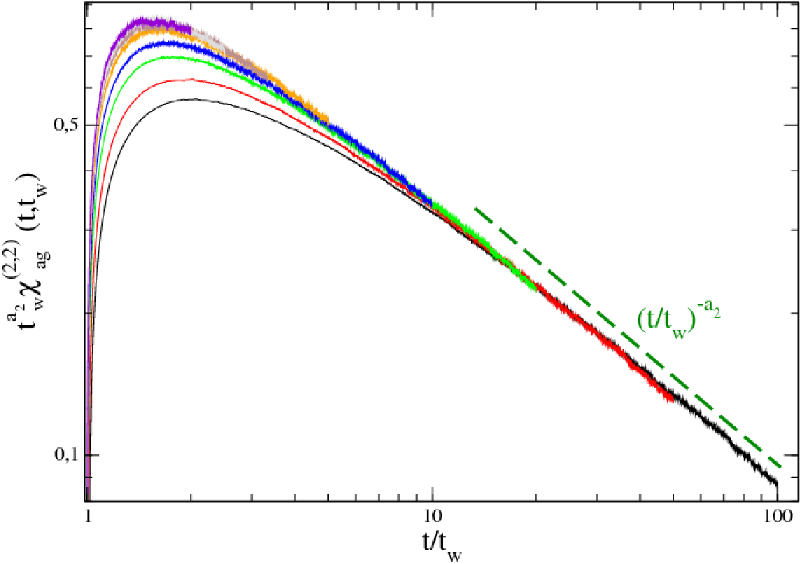
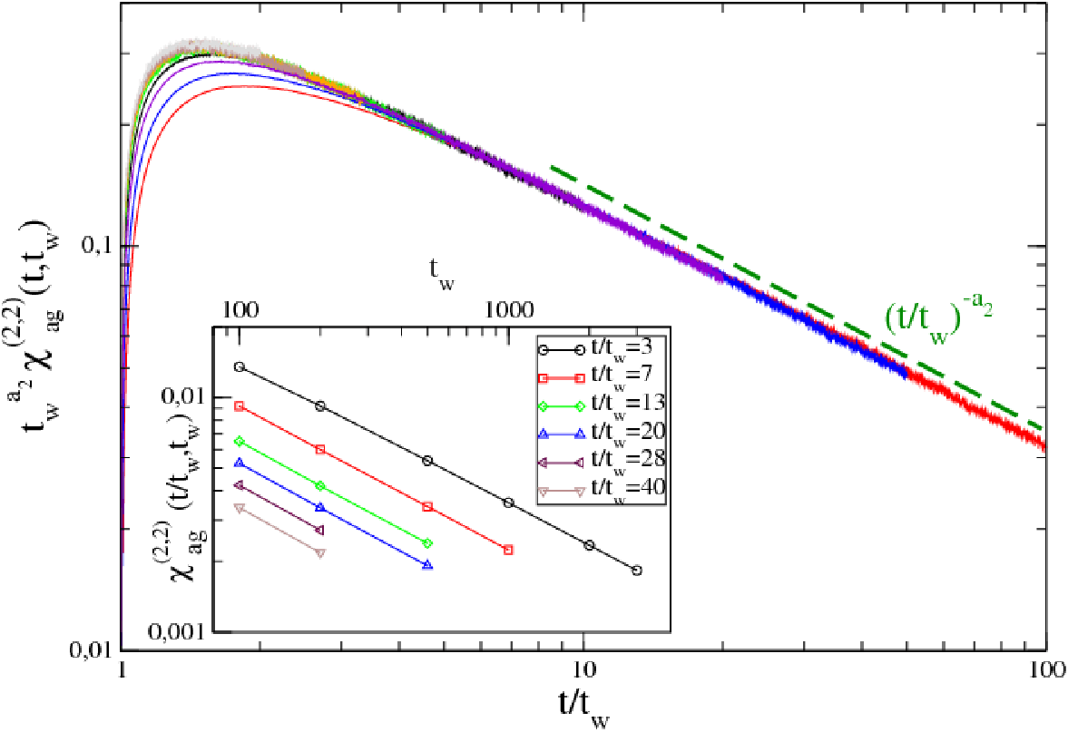
Figure 5: (Color online). twa2​χa​g(2,2)​(t,tw)t_{w}^{a_{2}}\chi^{(2,2)}_{ag}(t,t_{w}) is plotted against t/twt/t_{w} for tw=100,200,500,1000,2000,3000,4000,5000t_{w}=100,200,500,1000,2000,3000,4000,5000 (from bottom to top) and three temperatures T=1,1.5,2T=1,1.5,2 (upper, central and lower panel). The exponent a2a_{2} is extracted as discussed in the text, finding a2=0.61a_{2}=0.61 for T=1T=1, and a2=0.62a_{2}=0.62 for T=1.5T=1.5 and T=2T=2. The dashed lines represent the asymptotic behavior χa​g(2,2)​(t,tw)∼(t/tw)−a2\chi^{(2,2)}_{ag}(t,t_{w})\sim(t/t_{w})^{-a_{2}} for large t/twt/t_{w}. In the inset the quantity χa​g(2,2)​(t,tw)\chi^{(2,2)}_{ag}(t,t_{w}) is plotted against twt_{w} with t/twt/t_{w} fixed.

In order to check if a scaling form of the type (98) is obeyed

χa​g(2,2)​(ψ(2),tw)=tw−a2​F2​(t/tw)\chi^{(2,2)}_{ag}(\psi^{(2)},t_{w})=t_{w}^{-a_{2}}F_{2}(t/t_{w}) (107)

we have plotted χa​g(2,2)​(t,tw)\chi^{(2,2)}_{ag}(t,t_{w}) for a fixed value of t/twt/t_{w} against twt_{w}, as shown in the inset of the upper panel of Fig. 5. From the observed power law behavior we have extracted the exponent a2a_{2}, finding values in the range [0.59−0.62][0.59-0.62]. We have, then, carried out the data collapse by plotting twa2​χa​g(2)​(t,tw)t_{w}^{a_{2}}\chi^{(2)}_{ag}(t,t_{w}) against t/twt/t_{w}. For large twt_{w} the collapse (Fig. 5) is quite good, confirming that the scaling form (107) is obeyed with an exponent a2≃0.61−0.62a_{2}\simeq 0.61-0.62. For small values of twt_{w} and t/twt/t_{w} deviations are observed due to preasymptotic effects, similarly to what was already observed in the linear case [23, 27]. Notice, also, that for large t/twt/t_{w} one has a power law decay of the scaling function F2​(t/tw)∼(t/tw)−a2F_{2}(t/t_{w})\sim(t/t_{w})^{-a_{2}} with the same exponent a2a_{2} entering Eq. (107), exactly as it was observed in the linear case [27].

In conclusion, like in the linear case, the existence of the scaling behavior (107) with a2>0a_{2}>0 implies that the aging contribution vanishes asymptotically, yielding the analogue of Eq. (99)

limtw→∞χk→=0(2,2)​(ψ(2),tw)={β2​ψ(2),for​ψ(2)≤(1−Me​q2)2β2​(1−Me​q2)2,for​(1−Me​q2)2<ψ(2).\lim_{t_{w}\to\infty}\chi^{(2,2)}_{\vec{k}=0}(\psi^{(2)},t_{w})=\left\{\begin{array}[]{ll}\beta^{2}\psi^{(2)},\;\;$for$\;\;\psi^{(2)}\leq(1-M_{eq}^{2})^{2}\\ \beta^{2}(1-M_{eq}^{2})^{2},\;\;$for$\;\;(1-M_{eq}^{2})^{2}<\psi^{(2)}.\end{array}\right. (108)

The approach to this asymptotic behavior is shown in Fig. 6. Hence, using the definition (104), we find

limtw→∞βe​f​f​(ψ(2),tw)={β,for​ψ(2)≤(1−Me​q2)20,for​(1−Me​q2)2<ψ(2).\lim_{t_{w}\to\infty}\beta_{eff}(\psi^{(2)},t_{w})=\left\{\begin{array}[]{ll}\beta,\;\;$for$\;\;\psi^{(2)}\leq(1-M_{eq}^{2})^{2}\\ 0,\;\;$for$\;\;(1-M_{eq}^{2})^{2}<\psi^{(2)}.\end{array}\right. (109)

The comparison with Eq. (100) suggests that the consistency condition (105) is satisfied.

Refer to caption
Figure 6: (Color online). The parametric plot of χk=0(2,2)​(t,tw)\chi^{(2,2)}_{k=0}(t,t_{w}) against β2​ψ(2)\beta^{2}\psi^{(2)} (χi(1,1)​(t,tw)\chi^{(1,1)}_{i}(t,t_{w}) against β​ψ(1)\beta\psi^{(1)} in the inset) is shown for T=2T=2 and tw=100,200,500,1000,2000,3000,4000,5000t_{w}=100,200,500,1000,2000,3000,4000,5000, from top to bottom. The dashed line is the expected asymptotic behavior.

VIII Conclusions

In this paper we have derived the off equilibrium FDR of arbitrary order for systems evolving with Markovian stochastic dynamics. The main effort has been to put the FDR in the same form for both continous and discrete spins. In order to stress the generality of the result, we have also shown how the whole hierarchy of FDR can be made to descend from the fluctuation principle. Once the FDR are available, response functions of arbitrary order are expressed in terms of unperturbed correlation functions of observables. The payoff is in the development of simple and efficient zero field algorithms for the numerical simulations.

As an application, we have considered the problem of detecting the existence of a growing length in those cases, like in glassy systems, where standard methods based on two-point correlation functions and the corresponding linear response functions are of no use. In these cases the simplest object carrying useful information, in principle, would be a four-point correlation function which, however, is not directly accessible to experiment. Instead, experimentally accessible are the nonlinear response functions involving the four-point correlation function through the nonlinear FDR. The choice of which response function and, therefore, of which FDR to use is not univocal, once the realm of the nonlinear response functions is entered. Then the choice is matter of convenience. We have made the proposal to use the second order response of a two-point correlation function, rather than the third order response of the magnetization, as advocated elsewhere in the literature. We have, then, demonstrated the numerical advantage of our choice through the implementation of the zero field algorithm.

Finally, we have made a first step into the important but difficult problem of the definition of the effective temperature through the nonlinear FDR. We have considered the domain coarsening process ensuing the quench of a ferromagnet below its critical point. Indeed, in that case we have found that it is possible to extract from the nonlinear FDR an effective temperature which is consistent with the effective temperature obtained from the much studied linear FDR.

IX Appendix I

Proceeding like in the derivation of Eq. (26), the third order derivative of the propagator is given by

δ3​P^h​(t|tw)δ​hj1​(t1)​δ​hj2​(t2)​δ​hj3​(t3)=\displaystyle{\delta^{3}\hat{P}_{h}(t|t_{w})\over\delta h_{j_{1}}(t_{1})\delta h_{j_{2}}(t_{2})\delta h_{j_{3}}(t_{3})}= (110)
P^h​(t|tM)​∂W^​(tM)∂hjM​(tM)​P^h​(tM|tI)​∂W^​(tI)∂hjI​(tI)​P^h​(tI|tm)​∂W^​(tm)∂hjm​(tm)​P^h​(tm|tw)\displaystyle\hat{P}_{h}(t|t_{M}){\partial\hat{W}(t_{M})\over\partial h_{j_{M}}(t_{M})}\hat{P}_{h}(t_{M}|t_{I}){\partial\hat{W}(t_{I})\over\partial h_{j_{I}}(t_{I})}\hat{P}_{h}(t_{I}|t_{m}){\partial\hat{W}(t_{m})\over\partial h_{j_{m}}(t_{m})}\hat{P}_{h}(t_{m}|t_{w})
+\displaystyle+ P^h​(t|tM)​∂2W^​(tI)∂hjI2​(tI)​P^h​(tI|tm)​∂W^​(tm)∂hjm​(tm)​P^h​(tm|tw)​δjM,jI​δ​(tM−tI)\displaystyle\hat{P}_{h}(t|t_{M}){\partial^{2}\hat{W}(t_{I})\over\partial h^{2}_{j_{I}}(t_{I})}\hat{P}_{h}(t_{I}|t_{m}){\partial\hat{W}(t_{m})\over\partial h_{j_{m}}(t_{m})}\hat{P}_{h}(t_{m}|t_{w})\delta_{j_{M},j_{I}}\delta(t_{M}-t_{I})
+\displaystyle+ P^h​(t|tM)​∂W^​(tM)∂hjM​(tM)​P^h​(tM|tI)​∂2W^​(tI)∂hjI2​(tI)​P^h​(tI|tw)​δjI,jm​δ​(tI−tm)\displaystyle\hat{P}_{h}(t|t_{M}){\partial\hat{W}(t_{M})\over\partial h_{j_{M}}(t_{M})}\hat{P}_{h}(t_{M}|t_{I}){\partial^{2}\hat{W}(t_{I})\over\partial h^{2}_{j_{I}}(t_{I})}\hat{P}_{h}(t_{I}|t_{w})\delta_{j_{I},j_{m}}\delta(t_{I}-t_{m})
+\displaystyle+ P^h​(t|t1)​∂3W^​(t1)∂hj13​(t1)​P^h​(t1|tw)​δ​(12)​δ​(23)\displaystyle\hat{P}_{h}(t|t_{1}){\partial^{3}\hat{W}(t_{1})\over\partial h^{3}_{j_{1}}(t_{1})}\hat{P}_{h}(t_{1}|t_{w})\delta(12)\delta(23)

where tM=max⁡(tj)t_{M}=\max(t_{j}), tm=min⁡(tj)t_{m}=\min(t_{j}), tm≤tI≤tMt_{m}\leq t_{I}\leq t_{M}, jM,jI,jmj_{M},j_{I},j_{m} are the sites where the field acts at the times tMt_{M}, tIt_{I} or tmt_{m}, respectively, and δ⁡(n​p)=δjn,jp​δ​(tn−tp)\delta(np)=\delta_{j_{n},j_{p}}\delta(t_{n}-t_{p}). Inserting this into Eq. (24) and using Eq. (53), we get the third order response of the first moment

Ri;j1​j2​j3(1,3)(t,t1,t2,t3)=(β2)3{∂3∂tM​∂tI​∂tmMi​jM​jI​jm(t,tM,tI,tm)\displaystyle R^{(1,3)}_{i;j_{1}j_{2}j_{3}}(t,t_{1},t_{2},t_{3})=\left(\frac{\beta}{2}\right)^{3}\Big\{\frac{\partial^{3}}{\partial t_{M}\partial t_{I}\partial t_{m}}M_{ij_{M}j_{I}j_{m}}(t,t_{M},t_{I},t_{m}) (111)
−\displaystyle- ∂2∂tM​∂tI​⟨σ^i​(t)​σ^jM​(tM)​σ^jI​(tI)​B^jm​(tm)⟩−∂2∂tM​∂tm​⟨σ^i​(t)​σ^jM​(tM)​B^jI​(tI)​σ^jm​(tm)⟩\displaystyle\frac{\partial^{2}}{\partial t_{M}\partial t_{I}}\langle\hat{\sigma}_{i}(t)\hat{\sigma}_{j_{M}}(t_{M})\hat{\sigma}_{j_{I}}(t_{I})\hat{B}_{j_{m}}(t_{m})\rangle-\frac{\partial^{2}}{\partial t_{M}\partial t_{m}}\langle\hat{\sigma}_{i}(t)\hat{\sigma}_{j_{M}}(t_{M})\hat{B}_{j_{I}}(t_{I})\hat{\sigma}_{j_{m}}(t_{m})\rangle
−\displaystyle- ∂2∂tI​∂tm​⟨σ^i​(t)​B^jM​(tM)​σ^jI​(tI)​σ^jm​(tm)⟩+∂∂tm​⟨σ^i​(t)​B^jM​(tM)​B^jI​(tI)​σ^jm​(tm)⟩\displaystyle\frac{\partial^{2}}{\partial t_{I}\partial t_{m}}\langle\hat{\sigma}_{i}(t)\hat{B}_{j_{M}}(t_{M})\hat{\sigma}_{j_{I}}(t_{I})\hat{\sigma}_{j_{m}}(t_{m})\rangle+\frac{\partial}{\partial t_{m}}\langle\hat{\sigma}_{i}(t)\hat{B}_{j_{M}}(t_{M})\hat{B}_{j_{I}}(t_{I})\hat{\sigma}_{j_{m}}(t_{m})\rangle
+\displaystyle+ ∂∂tI​⟨σ^i​(t)​B^jM​(tM)​σ^jI​(tI)​B^jm​(tm)⟩+∂∂tM​⟨σ^i​(t)​σ^jM​(tM)​B^jI​(tI)​B^jm​(tm)⟩\displaystyle\frac{\partial}{\partial t_{I}}\langle\hat{\sigma}_{i}(t)\hat{B}_{j_{M}}(t_{M})\hat{\sigma}_{j_{I}}(t_{I})\hat{B}_{j_{m}}(t_{m})\rangle+\frac{\partial}{\partial t_{M}}\langle\hat{\sigma}_{i}(t)\hat{\sigma}_{j_{M}}(t_{M})\hat{B}_{j_{I}}(t_{I})\hat{B}_{j_{m}}(t_{m})\rangle
−\displaystyle- ⟨σi(t)BjM(tM)BjI(tI)Bjm(tm)⟩}+β34{(∂∂tm⟨σ^i(t)σ^jI(tI)B^jI(tI)σ^jm(tm)⟩\displaystyle\langle\sigma_{i}(t)B_{j_{M}}(t_{M})B_{j_{I}}(t_{I})B_{j_{m}}(t_{m})\rangle\Big\}+\frac{\beta^{3}}{4}\Big\{\Big(\frac{\partial}{\partial t_{m}}\langle\hat{\sigma}_{i}(t)\hat{\sigma}_{j_{I}}(t_{I})\hat{B}_{j_{I}}(t_{I})\hat{\sigma}_{j_{m}}(t_{m})\rangle
+\displaystyle+ ∂∂tm​∂∂tI​Mi​jM​jI​jm​(t,tM,tI,tm)−⟨σ^i​(t)​σ^jI​(tI)​B^jI​(tI)​B^jm​(tm)⟩\displaystyle\frac{\partial}{\partial t_{m}}\frac{\partial}{\partial t_{I}}M_{ij_{M}j_{I}j_{m}}(t,t_{M},t_{I},t_{m})-\langle\hat{\sigma}_{i}(t)\hat{\sigma}_{j_{I}}(t_{I})\hat{B}_{j_{I}}(t_{I})\hat{B}_{j_{m}}(t_{m})\rangle
−\displaystyle- OPEN∂∂tI​⟨σ^i​(t)​σ^jM​(tM)​σ^jI​(tI)​B^jm​(tm)⟩)​δjM​jI​δ​(tM−tI)+(∂∂tM​⟨σ^i​(t)​σ^jM​(tM)​σ^jI​(tI)​B^jI​(tI)⟩CLOSE\displaystyle\frac{\partial}{\partial t_{I}}\langle\hat{\sigma}_{i}(t)\hat{\sigma}_{j_{M}}(t_{M})\hat{\sigma}_{j_{I}}(t_{I})\hat{B}_{j_{m}}(t_{m})\rangle\Big)\delta_{j_{M}j_{I}}\delta(t_{M}-t_{I})+\Big(\frac{\partial}{\partial t_{M}}\langle\hat{\sigma}_{i}(t)\hat{\sigma}_{j_{M}}(t_{M})\hat{\sigma}_{j_{I}}(t_{I})\hat{B}_{j_{I}}(t_{I})\rangle
+\displaystyle+ ∂∂tM​∂∂tm​Mi​jM​jI​jm​(t,tM,tI,tm)−⟨σ^i​(t)​B^jM​(tM)​σ^jI​(tI)​B^jI​(tI)⟩\displaystyle\frac{\partial}{\partial t_{M}}\frac{\partial}{\partial t_{m}}M_{ij_{M}j_{I}j_{m}}(t,t_{M},t_{I},t_{m})-\langle\hat{\sigma}_{i}(t)\hat{B}_{j_{M}}(t_{M})\hat{\sigma}_{j_{I}}(t_{I})\hat{B}_{j_{I}}(t_{I})\rangle
−\displaystyle- ∂∂tm⟨σ^i(t)B^jM(tM)σ^jI(tI)σ^jm(tm)⟩)δjI​jmδ(tI−tm)}+β32(∂∂t1Mi​j1(t,t1)\displaystyle\frac{\partial}{\partial t_{m}}\langle\hat{\sigma}_{i}(t)\hat{B}_{j_{M}}(t_{M})\hat{\sigma}_{j_{I}}(t_{I})\hat{\sigma}_{j_{m}}(t_{m})\rangle\Big)\delta_{j_{I}j_{m}}\delta(t_{I}-t_{m})\Big\}+\frac{\beta^{3}}{2}\Big(\frac{\partial}{\partial t_{1}}M_{ij_{1}}(t,t_{1})
−\displaystyle- OPEN⟨σ^i​(t)​B^j1​(t1)⟩)​δj1​j2​δj2​j3​δ​(t1−t2)​δ​(t2−t3).\displaystyle\langle\hat{\sigma}_{i}(t)\hat{B}_{j_{1}}(t_{1})\rangle\Big)\delta_{j_{1}j_{2}}\delta_{j_{2}j_{3}}\delta(t_{1}-t_{2})\delta(t_{2}-t_{3}).

At stationarity this becomes

Ri​j1​j2​j3(1,3)​(t,t1,t2,t3)\displaystyle R^{(1,3)}_{ij_{1}j_{2}j_{3}}(t,t_{1},t_{2},t_{3}) =\displaystyle= β34{∂3∂tM​∂tI​∂tmMi​jM​jI​jm(t,tM,tI,tm)\displaystyle\frac{\beta^{3}}{4}\Big\{\frac{\partial^{3}}{\partial t_{M}\partial t_{I}\partial t_{m}}M_{ij_{M}j_{I}j_{m}}(t,t_{M},t_{I},t_{m})
−\displaystyle- ∂2∂tM​∂tm​⟨σ^i​(t)​σ^jM​(tM)​B^jI​(tI)​σ^jm​(tm)⟩\displaystyle\frac{\partial^{2}}{\partial t_{M}\partial t_{m}}\langle\hat{\sigma}_{i}(t)\hat{\sigma}_{j_{M}}(t_{M})\hat{B}_{j_{I}}(t_{I})\hat{\sigma}_{j_{m}}(t_{m})\rangle
−\displaystyle- ∂2∂tI​∂tm​⟨σ^i​(t)​B^jM​(tM)​σ^jI​(tI)​σ^jm​(tm)⟩\displaystyle\frac{\partial^{2}}{\partial t_{I}\partial t_{m}}\langle\hat{\sigma}_{i}(t)\hat{B}_{j_{M}}(t_{M})\hat{\sigma}_{j_{I}}(t_{I})\hat{\sigma}_{j_{m}}(t_{m})\rangle
+\displaystyle+ ∂∂tm⟨σ^i(t)B^jM(tM)B^jI(tI)σ^jm(tm)⟩}\displaystyle\frac{\partial}{\partial t_{m}}\langle\hat{\sigma}_{i}(t)\hat{B}_{j_{M}}(t_{M})\hat{B}_{j_{I}}(t_{I})\hat{\sigma}_{j_{m}}(t_{m})\rangle\Big\}
+\displaystyle+ β32{∂∂tm⟨σ^i(t)σ^jI(tI)B^jI(tI)σ^jm(tm)⟩\displaystyle\frac{\beta^{3}}{2}\Big\{\frac{\partial}{\partial t_{m}}\langle\hat{\sigma}_{i}(t)\hat{\sigma}_{j_{I}}(t_{I})\hat{B}_{j_{I}}(t_{I})\hat{\sigma}_{j_{m}}(t_{m})\rangle
+\displaystyle+ ∂∂tm∂∂tIMi​jM​jI​jm(t,tM,tI,tm)}δjM​jIδ(tM−tI)\displaystyle\frac{\partial}{\partial t_{m}}\frac{\partial}{\partial t_{I}}M_{ij_{M}j_{I}j_{m}}(t,t_{M},t_{I},t_{m})\Big\}\delta_{j_{M}j_{I}}\delta(t_{M}-t_{I})
+\displaystyle+ β3​∂∂t1​Mi​j1​(t,t1)​δj1​j2​δj2​j3​δ​(t1−t2)​δ​(t2−t3).\displaystyle\beta^{3}\frac{\partial}{\partial t_{1}}M_{ij_{1}}(t,t_{1})\delta_{j_{1}j_{2}}\delta_{j_{2}j_{3}}\delta(t_{1}-t_{2})\delta(t_{2}-t_{3}).

It should be recalled that the singular terms in the last two equations are present only in the Ising spin case.

X Appendix II

The expansion of the left hand side of Eq. (67) can be done in two steps. Expanding first the exponential we get

⟨φi(tF)exp{−β∫t0tFdth(t)φ˙(t)}⟩I→β,[h⁡(t)]\displaystyle\left\langle\varphi_{i}(t_{F})\exp\left\{-\beta\int_{t_{0}}^{t_{F}}dt\;h(t)\dot{\varphi}(t)\right\}\right\rangle_{I\rightarrow\beta,[h(t)]} (113)
=\displaystyle= ∑m=0∞(−β)mm!​∑j1​…​jm∫t0tFd​t1​…​d​tm​⟨φi​(tF)​φ˙j1​(t1)​…​φ˙jm​(tm)⟩I→β,[h⁡(t)]\displaystyle\sum_{m=0}^{\infty}{(-\beta)^{m}\over m!}\sum_{j_{1}...j_{m}}\int_{t_{0}}^{t_{F}}dt_{1}...dt_{m}\langle\varphi_{i}(t_{F})\dot{\varphi}_{j_{1}}(t_{1})...\dot{\varphi}_{j_{m}}(t_{m})\rangle_{I\rightarrow\beta,[h(t)]}
hj1​(t1)​…​hjm​(tm)\displaystyle h_{j_{1}}(t_{1})...h_{j_{m}}(t_{m})

and expanding the individual averages

⟨φi​(tF)​φ˙j1​(t1)​…​φ˙jm​(tm)⟩I→β,[h⁡(t)]=\displaystyle\langle\varphi_{i}(t_{F})\dot{\varphi}_{j_{1}}(t_{1})...\dot{\varphi}_{j_{m}}(t_{m})\rangle_{I\rightarrow\beta,[h(t)]}=
∑p=0∞1p!​∑q1​…​qp∫t0tFd​t1′​…​d​tp′​δp​⟨φi​(tF)​φ˙j1​(t1)​…​φ˙jm​(tm)⟩I→β,[h⁡(t)]δ​hq1​(t1′)​…​δ​hqp​(tp′)|h=0\displaystyle\sum_{p=0}^{\infty}{1\over p!}\sum_{q_{1}...q_{p}}\int_{t_{0}}^{t_{F}}dt_{1}^{\prime}...dt_{p}^{\prime}\left.{\delta^{p}\langle\varphi_{i}(t_{F})\dot{\varphi}_{j_{1}}(t_{1})...\dot{\varphi}_{j_{m}}(t_{m})\rangle_{I\rightarrow\beta,[h(t)]}\over\delta h_{q_{1}}(t_{1}^{\prime})...\delta h_{q_{p}}(t_{p}^{\prime})}\right|_{h=0}
hq1​(t1′)​…​hqp​(tp′)\displaystyle h_{q_{1}}(t_{1}^{\prime})...h_{q_{p}}(t_{p}^{\prime}) (114)

all together these two contributions give

⟨φi(tF)exp{−β∫t0tFdth(t)φ˙(t)}⟩I→β,[h⁡(t)]=\displaystyle\left\langle\varphi_{i}(t_{F})\exp\left\{-\beta\int_{t_{0}}^{t_{F}}dt\;h(t)\dot{\varphi}(t)\right\}\right\rangle_{I\rightarrow\beta,[h(t)]}=
∑m=0∞∑p=0∞(−β)mm!​p!​∑j1​…​jm∑q1​…​qp∫t0tFd​t1​…​d​tm​d​t1′​…​d​tp′​δp​⟨φi​(tF)​φ˙j1​(t1)​…​φ˙jm​(tm)⟩I→β,[h⁡(t)]δ​hq1​(t1′)​…​δ​hqp​(tp′)|h=0\displaystyle\sum_{m=0}^{\infty}\sum_{p=0}^{\infty}{(-\beta)^{m}\over m!p!}\sum_{j_{1}...j_{m}}\sum_{q_{1}...q_{p}}\int_{t_{0}}^{t_{F}}dt_{1}...dt_{m}dt_{1}^{\prime}...dt_{p}^{\prime}\left.{\delta^{p}\langle\varphi_{i}(t_{F})\dot{\varphi}_{j_{1}}(t_{1})...\dot{\varphi}_{j_{m}}(t_{m})\rangle_{I\rightarrow\beta,[h(t)]}\over\delta h_{q_{1}}(t_{1}^{\prime})...\delta h_{q_{p}}(t_{p}^{\prime})}\right|_{h=0}
hj1​(t1)​…​hjm​(tm)​hq1​(t1′)​…​hqp​(tp′).\displaystyle h_{j_{1}}(t_{1})...h_{j_{m}}(t_{m})h_{q_{1}}(t_{1}^{\prime})...h_{q_{p}}(t_{p}^{\prime}). (115)

Reorganizing the double sum

∑m=0∞∑p=0∞(−β)mm!​p!∑j1​…​jm∑q1​…​qp=∑n=0∞∑p=0n(−β)n−p(n−p)!​p!∑j1​…​jn−p∑q1​…​qp\sum_{m=0}^{\infty}\sum_{p=0}^{\infty}{(-\beta)^{m}\over m!p!}\sum_{j_{1}...j_{m}}\sum_{q_{1}...q_{p}}=\sum_{n=0}^{\infty}\sum_{p=0}^{n}{(-\beta)^{n-p}\over(n-p)!p!}\sum_{j_{1}...j_{n-p}}\sum_{q_{1}...q_{p}} (116)

the above result can be rewritten as

⟨φi(tF)exp{−β∫t0tFdth(t)φ˙(t)}⟩I→β,[h⁡(t)]=⟨φi(tF)⟩I→β,0\displaystyle\left\langle\varphi_{i}(t_{F})\exp\left\{-\beta\int_{t_{0}}^{t_{F}}dt\;h(t)\dot{\varphi}(t)\right\}\right\rangle_{I\rightarrow\beta,[h(t)]}=\langle\varphi_{i}(t_{F})\rangle_{I\rightarrow\beta,0}
∑n=1∞1n!​∑p=0n(−β)n−p​[n!(n−p)!​p!]​∑j1​…​jn−p∑q1​…​qp∫t0tFd​t1​…​d​tn−p​d​t1′​…​d​tp′\displaystyle\sum_{n=1}^{\infty}{1\over n!}\sum_{p=0}^{n}(-\beta)^{n-p}\left[{n!\over(n-p)!p!}\right]\sum_{j_{1}...j_{n-p}}\sum_{q_{1}...q_{p}}\int_{t_{0}}^{t_{F}}dt_{1}...dt_{n-p}dt_{1}^{\prime}...dt_{p}^{\prime}
δp​⟨φi​(tF)​φ˙j1​(t1)​…​φ˙jn−p​(tn−p)⟩I→β,[h⁡(t)]δ​hq1​(t1′)​…​δ​hqp​(tp′)|h=0​hj1​(t1)​…​hjn−p​(tn−p)​hq1​(t1′)​…​hqp​(tp′).\displaystyle\left.{\delta^{p}\langle\varphi_{i}(t_{F})\dot{\varphi}_{j_{1}}(t_{1})...\dot{\varphi}_{j_{n-p}}(t_{n-p})\rangle_{I\rightarrow\beta,[h(t)]}\over\delta h_{q_{1}}(t_{1}^{\prime})...\delta h_{q_{p}}(t_{p}^{\prime})}\right|_{h=0}h_{j_{1}}(t_{1})...h_{j_{n-p}}(t_{n-p})h_{q_{1}}(t_{1}^{\prime})...h_{q_{p}}(t_{p}^{\prime}).
(117)

Notice that the combinatorial factor in the square bracket gives the number of the distinct permutations among the two sets of indeces (j1,…,jn−p)(j_{1},...,j_{n-p}) and (q1,…,qp)(q_{1},...,q_{p}).

Going over to the right hand side of Eq. (67) and introducing the shorthand

⟨PI​(φ⁡(tF))​eβ​ℋ0​(φ⁡(tF))​φi​(t0)⟩β,0→β,[h~​(t)]=⟨R​H​S⟩β,0→β,[h~​(t)]\left\langle P_{I}(\varphi(t_{F}))e^{\beta{\cal H}_{0}(\varphi(t_{F}))}\varphi_{i}(t_{0})\right\rangle_{\beta,0\rightarrow\beta,[\widetilde{h}(t)]}=\langle RHS\rangle_{\beta,0\rightarrow\beta,[\widetilde{h}(t)]} (118)

one gets

⟨R​H​S⟩β,0→β,[h~​(t)]=⟨R​H​S⟩β,0\displaystyle\langle RHS\rangle_{\beta,0\rightarrow\beta,[\widetilde{h}(t)]}=\langle RHS\rangle_{\beta,0} (119)
+\displaystyle+ ∑n=1∞1n!​∑j1​…​jn∫t0tFd​t1​…​d​tn​δn​⟨R​H​S⟩β,0→β,[h~​(t)]δ​hj1​(t1)​…​δ​hjn​(tn)|h=0\displaystyle\sum_{n=1}^{\infty}{1\over n!}\sum_{j_{1}...j_{n}}\int_{t_{0}}^{t_{F}}dt_{1}...dt_{n}\left.{\delta^{n}\langle RHS\rangle_{\beta,0\rightarrow\beta,[\widetilde{h}(t)]}\over\delta h_{j_{1}}(t_{1})...\delta h_{j_{n}}(t_{n})}\right|_{h=0}
hj1​(t1)​…​hjn​(tn)\displaystyle h_{j_{1}}(t_{1})...h_{j_{n}}(t_{n})

and, since h~j​(t~)=hj​(t)\widetilde{h}_{j}(\widetilde{t})=h_{j}(t), this can be rewritten as

⟨R​H​S⟩β,0→β,[h~​(t)]=⟨R​H​S⟩β,0\displaystyle\langle RHS\rangle_{\beta,0\rightarrow\beta,[\widetilde{h}(t)]}=\langle RHS\rangle_{\beta,0} (120)
+\displaystyle+ ∑n=1∞1n!​∑j1​…​jn∫t0tFd​t1​…​d​tn​δn​⟨R​H​S⟩β,0→β,[h~​(t)]δ​h~j1​(t~1)​…​δ​h~jn​(t~n)|h=0\displaystyle\sum_{n=1}^{\infty}{1\over n!}\sum_{j_{1}...j_{n}}\int_{t_{0}}^{t_{F}}dt_{1}...dt_{n}\left.{\delta^{n}\langle RHS\rangle_{\beta,0\rightarrow\beta,[\widetilde{h}(t)]}\over\delta\widetilde{h}_{j_{1}}(\widetilde{t}_{1})...\delta\widetilde{h}_{j_{n}}(\widetilde{t}_{n})}\right|_{h=0}
hj1​(t1)​…​hjn​(tn)\displaystyle h_{j_{1}}(t_{1})...h_{j_{n}}(t_{n})

where ⟨⋅⟩β,0\langle\cdot\rangle_{\beta,0} stands for the equilibrium average at the temperature β\beta and without external field. Therefore, comparing with Eq. (117), one arrives at Eqs. (68) and (69).

References

  • [1] For a review see A.J.Bray, Adv.Phys. 43, 357 (1994).
  • [2] D.A. Huse, J.Appl.Phys. 64, 5776 (1988).
  • [3] J.P.Bouchaud and G.Biroli, Phys.Rev.B 72, 064204 (2005).
  • [4] L. Berthier, G. Biroli, J.P. Bouchaud, L.Cipelletti, D. El Masri, D. L Hôte,F. Ladieu and M. Pierno, Science 310, 1797 (2005).
  • [5] L.F.Cugliandolo and J.Kurchan, Phys.Rev.Lett. 71, 173 (1993); L.F.Cugliandolo and J.Kurchan, J.Phys.A: Math.Gen. 27, 5749 (1994); Philos.Mag. 71, 501 (1995); S.Franz, M. Mézard, G.Parisi and L.Peliti, Phys.Rev.Lett. 81, 1758 (1998); J.Stat.Phys. 97, 459 (1999); G.Parisi, F.Ricci-Tersenghi and J.J.Ruiz-Lorenzo, Eur. Phys. J. B 11, 317 (1999).
  • [6] L.F.Cugliandolo, J.Kurchan and G.Parisi, J.Phys. I France, 4, 1641 (1994).
  • [7] G.Semerjian, L.F.Cugliandolo and A.Montanari, J.Stat.Phys. 115, 493 (2004).
  • [8] J.Kurchan, J.Phys. A 31, 3719 (1998). For e reviews see F.Ritort, Nonequilibrium fluctuations in small systems: From physics to biology, arXiv: 0705.0455v1; U.Marini Bettolo Marconi, A.Puglisi, L.Rondoni and A.Vulpiani, Phys.Reports 461, 111 (2008).
  • [9] The zero field algorithm based on the FDR (56) was presented in E.Lippiello,F.Corberi and M.Zannetti, Phys.Rev.E 71, 036104 (2005). Zero field algorithms, different from ours, were previously proposed by C.Chatelain, J.Phys.A 36, 10739 (2003) and F.Ricci-Tersenghi, Phys.Rev.E 68, 065104(R) (2003).
  • [10] L.F.Cugliandolo, J.Kurchan and L.Peliti, Phys. Rev. E 55, 3898 (1997).
  • [11] L.P.Kadanoff and J.Swift, Phys. Rev. 165, 310 (1968); K.Kawasaki, Phase Transitions and Critical Phenomena vol. 2, ed. C.Domb and M.S.Green, p.443 (New York, Academic, 1972).
  • [12] See for instance Ref. [7], where the derivation of the Onsager relation is carried out for continous variables, but it works exactly in the same way also for Ising spins.
  • [13] R.J. Glauber, J.Math.Phys. 4, 294 (1963).
  • [14] E. Lippiello, F. Corberi, A. Sarracino, and M. Zannetti, Phys.Rev. B 77, 212201 (2008).
  • [15] C. Donati, S.C. Glotzer and P. Poole, Phys.Rev.Lett. 82, 5064 (1999); S. Franz, C. Donati, G. Parisi and S.C. Glotzer, Phil.Mag.B 79, 1827 (1999); S. Franz and G. Parisi, J.Phys.:Condens.Mat. 12, 6335 (2000). See also Ref. [3] for a discussion.
  • [16] See L.F.Cugliandolo, Heterogeneities and local fluctuations in glassy systems, cond-mat/0401506v1 and references quoted therein.
  • [17] T. Jorg, J. Lukic, E. Marinari and O.C. Martin, Phys.Rev.Lett. 96, 237205 (2006).
  • [18] H.G. Katzgraber, L.W. Lee and A.P. Young, Phys. Rev. B 70, 014417 (2004); H.G. Katzgraber, L.W. Lee and I.A. Campbell, Phys.Rev.B 75, 014412 (2007).
  • [19] H. Rieger, B. Steckemetz and M. Schreckenberg, Europhys. Lett. 27, 485 (1994); H.G. Katzgraber, and I.A. Campbell, Phys.Rev.B 72, 014462 (2005).
  • [20] S.Fielding and P.Sollich, Phys.Rev.Lett. 88, 050603 (2002); P. Calabrese and A. Gambassi, J.Stat.Mech., P07013 (2004).
  • [21] D.S. Fisher and D.A. Huse, Phys.Rev. B 38, 373 (1994).
  • [22] J.P.Bouchaud, L.F.Cugliandolo, J.Kurchan and M.Mezard, in Spin glasses and random fields, A.P.Young ed. (World Scientific, 1998); L.F.Cugliandolo, in Slow relaxation and non-equilibrium dynamics in condensed matter, Les Houches Session LXXVII, J.L.Barrat, J.Dalibard, J.Kurchan and M.V.Feigel’man eds., (Springer-Verlag, Heidelberg, 2002).
  • [23] The actual value of this exponent is controversial. Our results can be found in Ref. [24, 25]. What is uncontroversial, and what matters here, is that for d>1d>1 and for Ising spins a>0a>0.
  • [24] F. Corberi, E. Lippiello, and M. Zannetti, Phys. Rev. E 63, 061506 (2001); F. Corberi, E. Lippiello, and M. Zannetti, Phys. Rev. E 74, 041113 (2006).
  • [25] F. Corberi, E. Lippiello and M. Zannetti, Phys. Rev. E 72, 056103 (2005);
  • [26] F. Corberi, E. Lippiello, M. Zannetti, Eur. Phys. J. B 24 (2001), 359; F. Corberi, E. Lippiello, and M. Zannetti, Phys. Rev. E 74, 041106 (2006); R. Burioni, D. Cassi, F. Corberi, and A. Vezzani, Phys. Rev. Lett. 96, 235701 (2006); R. Burioni, D. Cassi, F. Corberi, and A. Vezzani, Phys. Rev. E 75, 011113 (2007).
  • [27] F. Corberi, E. Lippiello and M. Zannetti, Phys.Rev. E 68, 046131 (2003).