X-ray refractive index of laser-dressed atoms

Preprint: arXiv:0809.3249

Christian Buth Thanks: Present address: Department of Physics and Astronomy, Louisiana State University, Baton Rouge, Louisiana 70803, USA Affiliation: Argonne National Laboratory, Argonne, Illinois 60439, USA Robin Santra Affiliation: Argonne National Laboratory, Argonne, Illinois 60439, USA Affiliation: Department of Physics, University of Chicago, Chicago, Illinois 60637, USA

October 14, 2008

Abstract

We investigated the complex index of refraction in the x-ray regime of atoms in laser light. The laser (intensity up to $10^{13}\,{\rm{W/cm^{2}}}$ , wavelength $800\,{\rm{nm}}$ ) modifies the atomic states but, by assumption, does not excite or ionize the atoms in their electronic ground state. Using quantum electrodynamics, we devise an ab initio theory to calculate the dynamic dipole polarizability and the photoabsorption cross section, which are subsequently used to determine the real and imaginary part, respectively, of the refractive index. The interaction with the laser is treated nonperturbatively; the x-ray interaction is described in terms of a one-photon process. We numerically solve the resolvents involved using a single-vector Lanczos algorithm. Finally, we formulate rate equations to copropagate a laser and an x-ray pulse through a gas cell. Our theory is applied to argon. We study the x-ray polarizability and absorption near the argon $K$ edge over a large range of dressing-laser intensities. We find electromagnetically induced transparency (EIT) for x rays on the Ar $\,1s\to 4p$ pre-edge resonance. We demonstrate that EIT in Ar allows one to imprint the shape of an ultrafast laser pulse on a broader x-ray pulse (duration $100\,{\rm{ps}}$ , photon energy $3.2\,{\rm{keV}}$ ). Our work thus opens new opportunities for research with hard x-ray sources.

pacs

32.30.Rj, 32.80.Fb, 32.80.Rm, 42.50.Hz

I Introduction

We study the interaction of atoms with two-color light. Specifically, we consider an optical laser with moderate intensity and x rays. In experiments this light would be obtained, for instance, from an amplified Ti:sapphire laser system with up to $10^{13}\,$ W/cm² at a wavelength of $800\,{\rm{nm}}$ . The x rays would be produced by a third-generation synchrotron radiation source like Argonne’s Advanced Photon Source [1].

There are several ways for the chronology between the two light pulses. First, there is a pump-probe setting where the laser pulse precedes the x rays. Especially the combination of a weak laser as a pump and the x rays as a probe has received a lot of attention, e.g., Ref. 2. For higher laser intensities, ionization of atoms takes place, producing aligned, unoccupied atomic orbitals. They are probed by using xuv light or x rays to excite an inner-shell electron into them [3, 4, 5, 6]. Second, there is a pump-probe setting where the laser pulse succeeds the x rays. This situation has not received much of a focus (see, however, Ref. 7). Third, there is a simultaneous exposition of atoms and molecules to two colors. Recently, we studied molecules exposed to a laser with an intensity close to but still below the excitation and ionization threshold. If the molecule has an anisotropic polarizability tensor, they may be aligned along the linear laser polarization axis [6, 8, 9, 10, 11]; the x rays serve as an in situ probe of the rotational molecular dynamics. Going a bit higher in laser intensity, without exciting and ionizing, is possible for rare gas atoms. In krypton, laser dressing caused a pronounced deformation of the photoabsorption cross section around the $K$ edge [12, 6]. In neon we even found a strong suppression of the x-ray absorption on the Ne $\,1s\to 3p$ resonance [13, 6, 14, 11].

The name electromagnetically induced transparency (EIT) [15, 16, 17] for x rays was coined to describe the strong reduction of absorption in neon. It is related to EIT for optical wavelengths [18, 19, 20, 21, 22] by being essentially given by the same $\Lambda$ -type three-level model. The only difference in the case of EIT for x rays is the linewidth of the second unoccupied level which is not approximately zero. Due to high laser intensity, transparency over a large number of wavelengths arises. The difference between the x-ray absorption spectra for laser-dressed neon and krypton is predominantly due to the ten times higher decay width of the $K$ vacancies in krypton ( $\Gamma_{\mathrm{1s}}=2.7\,{\rm{eV}}$ [23, 24]) compared with neon ( $\Gamma_{\mathrm{1s}}=0.27\,{\rm{eV}}$ [25]). $K$ vacancies are produced by x-ray absorption and decay by x-ray fluorescence and Auger decay [1]. Another difference between EIT for optical wavelengths and EIT for x rays lies in the fact that refraction and dispersion by matter in the x-ray regime is generally tiny.

EIT enables ultrafast control of the absorption and dispersion of a gaseous medium on a femtosecond time scale because the coupling laser, typically a Ti:sapphire laser system, can be combined with the sophisticated pulse shaping technologies available for optical wavelengths [26]. These pulse shapes can be imprinted on x rays leading to ultrafast pulse shaping technology for x rays [13, 6, 14, 11]. The ability to create almost arbitrarily shaped x-ray pulses opens up perspectives for the control of the dynamics of the inner-shell electrons in atoms. This way of shaping x-ray pulses is similar to our recent study of x-ray absorption by laser-aligned molecules where x-ray pulses are shaped by controlling the molecular alignment [10]. As the rotational dynamics of molecules takes place on a picosecond time scale, the x-ray pulse shaping is, however, done on a much slower time scale. Electron bunch manipulation techniques for short x-ray pulse generation are presently developed at synchrotron radiation facilities [27]. Our approach complements these efforts in a very cost-effective way.

In this work, we would like to supplement our previous investigations with a detailed account of the refraction and the dispersion of x rays by laser-dressed atoms. Our theory is applied to argon. Also we demonstrate that there is appreciable EIT for x rays for argon. As there is no substantial EIT effect for krypton, this means that EIT for hard x rays is predicted for the first time (the $K$ electrons of argon can be ionized with x rays of a wavelength of $3.9\,{\rm{\hbox{\AA}}}$ [1]). Such wavelengths are already useful to resolve coarse molecular structures via x-ray diffraction in molecular imaging; our work offers a way of temporal control of the x-ray pulses in such experiments.

The paper is structured as follows. In Sec. II, we evolve our quantum electrodynamic formalism of Ref. 12 to incorporate rudimentary many-electron effects. We determine the dynamic dipole polarizability for x rays and the x-ray absorption cross section in Secs. II.1, II.2, and II.3 on an ab initio level. Resolvents are evaluated in Sec. II.4 with a single-vector Lanczos algorithm. Using these quantities together with the classical Maxwell equations in Sec. II.5, we devise the complex index of refraction for x rays of laser-dressed atoms. The propagation of pulses through this new medium is treated in Sec. II.6. Computational details are given in Sec. III for the results which are presented in Sec. IV. Conclusions are drawn in Sec. V. Finally, secondary physical processes of the pulse propagation from Sec. II.6 are treated in the appendix.

Our equations are formulated in atomic units [28]. The Bohr radius $1\,{\rm{bohr}}=1\,a_{0}$ is the unit of length and $1\,t_{0}$ represents the unit of time. The unit of energy is $1\,{\rm{hartree}}=1\,{\rm{E_{\mathit{h}}}}$ . Intensities are given in units of $1\,{\rm{E_{\mathit{h}}}}\>t_{0}^{-1}\,a_{0}^{-2}=6.43641\times 10^{15}\,{\rm{W\,cm^{-2}}}$ . Electric polarizabilities are measured in $1\,e^{2}\,a_{0}^{2}\,\,{\rm{E_{\mathit{h}}}}^{-1}=1.64878\times 10^{-41}\,{\rm{C^{2}\,m^{2}\,J^{-1}}}$ . The dielectric constant of the vacuum is $\varepsilon_{0}={1\over 4\pi}$ .

II Theory

II.1 Atoms in an electromagnetic field

The time-independent Schrödinger equation of the field-free atom is

\hat{H}_{\mathrm{AT}}\,\Psi^{Z}_{s}(\vec{r}_{1}\,\sigma_{1},\ldots,\vec{r}_{Z}\,\sigma_{Z},t)=E_{s}\,\Psi^{Z}_{s}(\vec{r}_{1}\,\sigma_{1},\ldots,\vec{r}_{Z}\,\sigma_{Z},t)\;.

(1)

Here, $\hat{H}_{\mathrm{AT}}$ is the electronic Hamiltonian of the atom which contains the Coulomb interaction of the $Z$ atomic electrons with the nucleus and the two-particle interaction among the electrons [28, 29]. The wave functions $\Psi^{Z}_{s}(\vec{r}_{1}\,\sigma_{1},\ldots,\vec{r}_{Z}\,\sigma_{Z},t)$ with eigenenergy $E_{s}$ represent the ground state ( $s=0$ ) and core-excited excited states ( $s\geq 1$ ) of the atom [30] for the $u$ th electron at position $\vec{r}_{u}$ with spin projection quantum number $\sigma_{u}$ for $u\in\{1,\ldots,Z\}$ .

The free electromagnetic field is represented by the Hamiltonian

\hat{H}_{\mathrm{EM}}&=\sum\limits_{\vec{k}}\sum\limits_{\lambda=1}^{2}\hat{H}_{\mathrm{EM},\vec{k},\lambda}\;,\\ \hat{H}_{\mathrm{EM},\vec{k},\lambda}=\omega^{\vphantom{{\dagger}}}_{\vec{k}}\,\hat{a}^{{\dagger}}_{\vec{k},\lambda}\hat{a}^{\vphantom{{\dagger}}}_{\vec{k},\lambda}-N^{\vphantom{{\dagger}}}_{\vec{k},\lambda}\,\omega^{\vphantom{{\dagger}}}_{\vec{k}}\;,

(2)

where $\hat{a}^{{\dagger}}_{\vec{k},\lambda}$ and $\hat{a}^{\vphantom{{\dagger}}}_{\vec{k},\lambda}$ denote creation and annihilation operators, respectively, of photons in the mode $\vec{k},\lambda$ with wave vector $\vec{k}$ , polarization index $\lambda$ , and energy $\omega_{\vec{k}}$ [31]. Here, $N_{\vec{k},\lambda}$ indicates the number of photons in the mode $\vec{k},\lambda$ of some initial state. The energy of the initial state, Eq. (10) in our case, has been adjusted such that the field energy is zero. This simplifies our equations notably. However, physical quantities are of course independent of the absolute energy shift in Eq. (2).

We consider in this paper only two modes for the electromagnetic field denoted by L and X for the laser and the x rays, respectively. The eigenstates of the free electromagnetic field $\hat{H}_{\mathrm{EM}}$ are Fock number states

\left|\right.\!N_{\mathrm{L}}\!\left.\right>\otimes\left|\right.\!N_{\mathrm{X}}\!\left.\right>=(\hat{a}_{\mathrm{L}}^{{\dagger}})^{N_{\mathrm{L}}}\,(\hat{a}_{\mathrm{X}}^{{\dagger}})^{N_{\mathrm{X}}}\,\left|\right.\!0\!\left.\right>\;,

(3)

with the vacuum state $\left|\right.\!0\!\left.\right>$ .

The interaction of electrons with light is described by

\hat{H}_{\mathrm{I}}=\sum\limits_{\sigma=-{1\over 2}}^{{1\over 2}}\ \int\limits_{\mathbb{R}^{3}}\hat{\psi}_{\sigma}^{\dagger}(\vec{r})\;[\hat{\vec{p}}\cdot\vec{A}(\vec{r})+{\displaystyle{1}\over\displaystyle{2}}\,\vec{A}^{2}(\vec{r})]\;\hat{\psi}_{\sigma}(\vec{r})\>\mathrm{d}^{3}r\;,

(4)

using the principle of minimal coupling to the electromagnetic field [31, 32]. The field is represented by the vector potential $\vec{A}(\vec{r})$ for which we assume the Coulomb gauge. The electrons are created and annihilated by the field operators $\hat{\psi}_{\sigma}^{\dagger}(\vec{r})$ and $\hat{\psi}_{\sigma}(\vec{r})$ , respectively [29]. We assume that both laser and x-ray wavelengths are sufficiently large for the electric dipole approximation to be adequate. Then, the vector potential becomes independent of $\vec{r}$ .

In dipole approximation, the form (4) of the interaction Hamiltonian with the x rays reads

\hat{H}_{\mathrm{I,X}}=\sum\limits_{\sigma=-{1\over 2}}^{{1\over 2}}\ \int\limits_{\mathbb{R}^{3}}\hat{\psi}_{\sigma}^{\dagger}(\vec{r})\>[\hat{\vec{p}}\cdot\vec{A}_{\mathrm{X}}+{\displaystyle{1}\over\displaystyle{2}}\vec{A}_{\mathrm{X}}^{2}]\>\hat{\psi}_{\sigma}(\vec{r})\>\mathrm{d}^{3}r\;,

(5)

using the following mode expansion for the quantized vector potential of the x rays [31]:

\vec{A}_{\mathrm{X}}=\sqrt{{2\pi\over V\,\omega_{\mathrm{X}}}}\;[\vec{e}_{\mathrm{X}}\,\hat{a}_{\mathrm{X}}+\vec{e}_{\mathrm{X}}^{\,*}\,\hat{a}_{\mathrm{X}}^{\dagger}]\;.

(6)

It is frequently referred to as velocity form [33].

In laser physics, one typically transforms the interaction (4) in dipole approximation to the so-called length form. This can, of course, be accomplished either for the Hamiltonian with semiclassical electromagnetic fields [33] or, as in our case, in the quantum electrodynamic framework [31]. Then, the interaction Hamiltonian with the laser field becomes

\hat{H}_{\mathrm{I,L}}=\sum\limits_{\sigma=-{1\over 2}}^{{1\over 2}}\ \int\limits_{\mathbb{R}^{3}}\hat{\psi}_{\sigma}^{\dagger}(\vec{r})\>\vec{r}\cdot\vec{E}_{\mathrm{L}}\>\hat{\psi}_{\sigma}(\vec{r})\>\mathrm{d}^{3}r\;,

(7)

where we use the quantized mode expansion

\vec{E}_{\mathrm{L}}={\rm i}\,\sqrt{{2\pi\,\omega_{\mathrm{L}}\over V}}\;[\vec{e}_{\mathrm{L}}\,\hat{a}_{\mathrm{L}}-\vec{e}^{\,*}_{\mathrm{L}}\,\hat{a}_{\mathrm{L}}^{\dagger}]

(8)

for the electric field of the laser mode [31]. The influence of the two-color light (4) in dipole approximation has been decomposed into $\hat{H}_{\mathrm{I}}=\hat{H}_{\mathrm{I,L}}+\hat{H}_{\mathrm{I,X}}$ [Eqs. (5) and (7)].

The full Hamiltonian of an atom in two-color light $\hat{H}=\hat{H}_{0}+\hat{H}_{1}$ consists of a strongly interacting part [12]

\hat{H}_{0}&=\hat{H}_{\mathrm{0,L}}+\hat{H}_{\mathrm{0,X}}\;,\\ \hat{H}_{\mathrm{0,L}}=\hat{H}_{\mathrm{AT}}+\hat{H}_{\mathrm{EM,L}}+\hat{H}_{\mathrm{I,L}}\;,\\ \hat{H}_{\mathrm{0,X}}=\hat{H}_{\mathrm{EM,X}}\;,

(9)

and a weak perturbation due to the interaction with the x rays, $\hat{H}_{1}=\hat{H}_{\mathrm{I,X}}$ [12].

II.2 Dynamic Stark effect

We would like to determine the energy of the $K$ -shell electrons in the two-color field. It is given by a perturbative expansion with respect to the x-ray field using a basis of laser-dressed energy levels of the atom. The initial state of the atom in light is given by the direct product of the electronic ground state wave function and the Fock states for the laser and the x-ray mode

\left|\right.\!i\!\left.\right>&=\left|\right.\!\Psi^{Z}_{0}\!\left.\right>\otimes\left|\right.\!N_{\mathrm{L}}\!\left.\right>\;,\\ \left|\right.\!I\!\left.\right>=\left|\right.\!i\!\left.\right>\otimes\left|\right.\!N_{\mathrm{X}}\!\left.\right>\;.

(10)

The energy of the initial state is $E_{I,0}=\left<\right.\!I\!\left.\right|\hat{H}_{0}\left|\right.\!I\!\left.\right>$ . We assume that the electronic ground state of the atom is not noticeably altered by the light. Core-excited states with a vacancy in the $K$ shell serve as final states for x-ray absorption and emission. We define for $s\neq 0$ :

\left|\right.\!\Phi_{s,\mu}\!\left.\right>&=\left|\right.\!\Psi_{s}^{Z}\!\left.\right>\otimes\left|\right.\!N_{\mathrm{L}}-\mu\!\left.\right>\;,\\ \left|\right.\!\Phi^{\pm}_{s,\mu}\!\left.\right>=\left|\right.\!\Phi_{s,\mu}\!\left.\right>\otimes\left|\right.\!N_{\mathrm{X}}\pm 1\!\left.\right>\;.

(11)

Let us solve the strongly interacting laser-only problem (9) first in terms of a non-Hermitian, complex-symmetric representation of the Hamiltonian [34, 35, 36], using the laser-only basis (11) for $s,s^{\prime}\neq 0$ :

(\hbox{\boldmath{$H$}\unboldmath}_{\mathrm{0,L}})_{s,\mu;s^{\prime},\mu^{\prime}}=\left<\right.\!\Phi_{s,\mu}\!\left.\right|\hat{H}_{\mathrm{0,L}}\left|\right.\!\Phi_{s^{\prime},\mu^{\prime}}\!\left.\right>\;.

(12)

The eigenstates $\left|\right.\!F\!\left.\right>$ of Eq. (12) form the laser-dressed atomic energy levels with complex eigenenergies $E_{F}$ .

The interaction with the x-ray field is treated as a perturbation of the laser-free atomic ground state; the impact of the laser dressing arises exclusively in the final states. The full basis states that include the x rays are defined in Eq. (11); the laser-dressed atomic levels are given by the direct product states $\left|\right.\!F^{\pm}\!\left.\right>=\left|\right.\!F\!\left.\right>\otimes\left|\right.\!N_{\mathrm{X}}\pm 1\!\left.\right>$ which correspond to the energies $E_{F}^{\pm}=\left<\right.\!F^{\pm}\!\left.\right|\hat{H}_{0}\left|\right.\!F^{\pm}\!\left.\right>=E_{F}\pm\omega_{\mathrm{X}}$ . We use non-Hermitian perturbation theory [37, 12] to determine the complex energy

E_{\mathrm{res}}=E_{\mathrm{R}}-{\rm i}\,\Gamma/2

(13)

of the initial state (10), the so-called Siegert energy [34, 38]. The real part is the energy shift of the atomic level due to the laser and x-ray fields [39, 37] whereas $\Gamma$ stands for the transition rate from the initial state to Rydberg states or the continuum. The energy (13) is obtained from

\begin{array}[]{rcl}\displaystyle E_{I}&=&\displaystyle E_{I,0}+\underbrace{\left<\right.\!I\!\left.\right|\hat{H}_{1}\left|\right.\!I\!\left.\right>}_{P_{1}(\omega_{\mathrm{X}})}\\[21.52771pt] &&\displaystyle{}+\underbrace{\sum_{F}\sum_{s\in\{+,-\}}{\left<\right.\!I\!\left.\right|\hat{H}_{1}\left|\right.\!F^{s}\!\left.\right>\left<\right.\!F^{s}\!\left.\right|\hat{H}_{1}\left|\right.\!I\!\left.\right>\over E_{I,0}-E_{F}^{s}}}_{P_{2}(\omega_{\mathrm{X}})}\;.\end{array}

(14)

Assuming $N_{\mathrm{X}}\gg 1$ , the interaction matrix elements $\left<\right.\!I\!\left.\right|\hat{H}_{1}\left|\right.\!F^{+}\!\left.\right>$ and $\left<\right.\!I\!\left.\right|\hat{H}_{1}\left|\right.\!F^{-}\!\left.\right>$ are approximately the same.

The first order correction $P_{1}(\omega_{\mathrm{X}})$ in Eq. (14) is found by combining Eqs. (5), (6), and (10):

\begin{array}[]{rcl}\displaystyle P_{1}(\omega_{\mathrm{X}})&=&\displaystyle{1\over 2}\,\left<\right.\!I\!\left.\right|\sum\limits_{\sigma=-{1\over 2}}^{{1\over 2}}\ \int\limits_{\mathbb{R}^{3}}\hat{\psi}_{\sigma}^{\dagger}(\vec{r})\>\vec{A}^{2}_{\mathrm{X}}\>\hat{\psi}_{\sigma}(\vec{r})\>\mathrm{d}^{3}r\left|\right.\!I\!\left.\right>\\ &=&\displaystyle{\pi\,Z\over V\,\omega_{\mathrm{X}}}\,(2\,N_{\mathrm{X}}+1)\approx{2\pi\over V\,\omega_{\mathrm{X}}}\,N_{\mathrm{X}}\,Z\;.\end{array}

(15)

The one-particle operator $\vec{A}^{2}_{\mathrm{X}}$ hereby acts on all $Z$ electrons in the initial state (10). The tiny correction ${\pi\,Z\over V\,\omega_{\mathrm{X}}}$ after the second equals sign vanishes upon taking the limit $V\to\infty$ in the end. The real quantity $P_{1}(\omega_{\mathrm{X}})$ in Eq. (15) is the energy shift due to the scattering of x rays and represents the ac Stark shift [40, 37]. We find the corresponding dynamic polarizability [40] from

{\mathrm{Re}\,}P_{1}(\omega_{\mathrm{X}})=-{1\over 4}\,\alpha_{1}(\omega_{\mathrm{X}})\,E_{\mathrm{X,0}}^{2}\;.

(16)

The peak electric field of the x rays is $E_{\mathrm{X,0}}=\sqrt{8\pi\,\alpha\,I_{\mathrm{X}}}$ [33, 41] for the x-ray intensity $I_{\mathrm{X}}$ . From Eqs. (15) and (16), we obtain the first order atomic polarizability

\alpha_{1}(\omega_{\mathrm{X}})=-{Z\over\omega_{\mathrm{X}}^{2}}\;.

(17)

In analogy to Eq. (16), we define the second order contribution to the dynamic polarizability [40]. With the real part of $P_{2}(\omega_{\mathrm{X}})$ in Eq. (14), the well-known Kramers-Heisenberg form

\begin{array}[]{rcl}\displaystyle\alpha_{2}(\omega_{\mathrm{X}})&=&\displaystyle-{\displaystyle{4}\over\displaystyle{E_{\mathrm{X,0}}^{2}}}\ {\mathrm{Re}\,}P_{2}(\omega_{\mathrm{X}})\\ &=&\displaystyle{\displaystyle{4}\over\displaystyle{E_{\mathrm{X,0}}^{2}}}\ {\mathrm{Re}\,}\sum\limits_{F}\left<\right.\!I\!\left.\right|\hat{H}_{1}\left|\right.\!F^{+}\!\left.\right>\,\left<\right.\!F^{+}\!\left.\right|\hat{H}_{1}\left|\right.\!I\!\left.\right>\\ &&\displaystyle\hskip 50.00008pt{}\times\,{\displaystyle{2\,(E_{F}-E_{I,0})}\over\displaystyle{(E_{F}-E_{I,0})^{2}-\omega^{2}_{\mathrm{X}}}}\end{array}

(18)

results [31, 40].

Using the first and second order atomic polarizabilities from Eqs. (17) and (18), we can define the total atomic polarizability

\alpha_{\mathrm{I}}(\omega_{\mathrm{X}})=\alpha_{1}(\omega_{\mathrm{X}})+\alpha_{2}(\omega_{\mathrm{X}})\;.

(19)

We derive explicit equations for the polarizability $\alpha_{2}(\omega_{\mathrm{X}})$ in the next section.

II.3 Hartree-Fock-Slater approximation

We solve the Schrödinger equation (1) with the help of the independent-electron approximation [28, 29, 12]. Then, the $Z$ -electron ground-state wave function is given by a Slater determinant of one-electron orbitals $\Phi^{Z}_{0}(\vec{r}_{1}\,\sigma_{1},\ldots,\vec{r}_{Z}\,\sigma_{Z})$ . Using the formalism of second quantization, we have

\left|\right.\!\Phi^{Z}_{0}\!\left.\right>=\prod_{n,l,m\ \mathrm{occupied}}\hat{b}^{\dagger}_{n,l,m,\uparrow}\,\hat{b}^{\dagger}_{n,l,m,\downarrow}\left|\right.\!0\!\left.\right>

(20)

for a closed-shell atom. Here, $\hat{b}^{\dagger}_{n,l,m,\uparrow}$ and $\hat{b}^{\dagger}_{n,l,m,\downarrow}$ are creators of electrons in the spatial orbital $\varphi_{n,l,m}(\vec{r})$ with spin projection quantum number up ( $\sigma={1\over 2}={\uparrow}$ ) and down ( $\sigma=-{1\over 2}={\downarrow}$ ), respectively. The spatial orbitals are eigenfunctions of the one-electron Hamiltonian

\hat{H}_{\mathrm{HFS}}=-{1\over 2}\,\vec{\nabla}^{2}+V_{\mathrm{HFS}}(r)\;.

(21)

They are characterized by the principal quantum number $n$ , the angular momentum $l$ , and the magnetic quantum number $m$ [29]. To determine the effective one-electron central potential $V_{\mathrm{HFS}}(r)$ , we made the Hartree-Fock-Slater mean-field approximation [42, 43].

When x rays are absorbed, an electron may be ejected into the continuum leaving a core hole behind [44]. We use a complex absorbing potential (CAP) to handle such continuum electrons. The CAP is a one-particle operator which is added to $\hat{H}_{\mathrm{HFS}}$ . It is derived from smooth exterior complex scaling [45, 46, 47, 12]. Additionally, one needs to allow for the relaxation of core holes by x-ray fluorescence and Auger decay [1, 48] with a decay width of $\Gamma_{\mathrm{1s}}$ . According to Eq. (13), this is accounted for by adding $-{\rm i}\,\Gamma_{\mathrm{1s}}/2$ to all energies of core-excited states [12]. Subsuming these contributions, we obtain the effective one-electron atomic Hamiltonian [12] which we use instead of $\hat{H}_{\mathrm{AT}}$ in Eq. (9).

With the help of the spin orbitals, we can expand the field operators [29] in the equations of Secs. II.1 and II.2 as follows

\hat{\psi}_{\sigma}(\vec{r})&=\sum\limits_{n,l,m}\varphi_{n,l,m}(\vec{r})\>\hat{b}_{n,l,m,\sigma}\;,\\ \hat{\psi}_{\sigma}^{\dagger}(\vec{r})=\sum\limits_{n,l,m}\varphi^{*}_{n,l,m}(\vec{r})\>\hat{b}^{\dagger}_{n,l,m,\sigma}\;.

(22)

Based on the independent-particle ground state (20), we construct the spin-singlet $K$ -shell-excited states [28, 29]:

\left|\right.\!\Phi_{n,l,m,\mu}\!\left.\right>&={\displaystyle{1}\over\displaystyle{\sqrt{2}}}\>[\hat{b}^{\dagger}_{n,l,m,\uparrow}\>\hat{b}^{\vphantom{\dagger}}_{1,0,0,\uparrow}\\ \hskip 20.00003pt{}+\hat{b}^{\dagger}_{n,l,m,\downarrow}\>\hat{b}^{\vphantom{\dagger}}_{1,0,0,\downarrow}]\left|\right.\!\Phi^{Z}_{0}\!\left.\right>\\ {}\otimes\left|\right.\!N_{\mathrm{L}}-\mu\!\left.\right>\;,\\ \left|\right.\!\Phi^{\pm}_{n,l,m,\mu}\!\left.\right>=\left|\right.\!\Phi_{n,l,m,\mu}\!\left.\right>\otimes\left|\right.\!N_{\mathrm{X}}\pm 1\!\left.\right>\;,

(23)

as basis states [see Eq. (11)]. Note that $m$ is a conserved quantum number because the laser is linearly polarized; thus the matrix (12) blocks with respect to $m$ . Following Ref. 12, the Kramers-Heisenberg form (18) becomes

\begin{array}[]{rcl}\displaystyle\alpha_{2}(\omega_{\mathrm{X}},\vartheta_{\mathrm{LX}})&=&\displaystyle{2\over 3}\ {\mathrm{Re}\,}\biggl[\sum\limits_{m=-1}^{1}\varkappa_{m}(\vartheta_{\mathrm{LX}})\\ &&\displaystyle\hskip 22.0pt{}\times\sum\limits_{F}{(d_{F}^{(m)})^{2}\over E_{F}^{(m)}-E_{1s}-\omega_{\mathrm{X}}}\biggr]\;.\end{array}

(24)

Here, we omit the emission term “ $+$ ” which results from decomposing the denominator of Eq. (18) to emphasize the similarity to the expression for the cross section. The initial-state energy is the $K$ -shell energy $E_{I,0}=E_{1s}$ . The angular dependence of the polarizability (24) is given by $\varkappa_{m}(\vartheta_{\mathrm{LX}})$ which is equal to $\cos^{2}\vartheta_{\mathrm{LX}}$ for $m=0$ and equal to ${1\over 2}\sin^{2}\vartheta_{\mathrm{LX}}$ for $m=\pm 1$ . The radial dipole matrix elements are given by $d_{F}^{(m)}$ [12].

II.4 Lanczos solution of the polarizability

The full diagonalization of the interaction of the atom with the laser to obtain the new energy levels of a laser-dressed atom becomes impractical for larger numbers of atomic orbitals and photons. To be able to solve the equations for the polarizability (24) and the cross section [12] with acceptable computational effort, we employ a single-vector Lanczos algorithm [49, 50]. A real symmetric version has been implemented by Meyer and Pal [51]; it was extended to complex symmetric matrices by Sommerfeld et al. [52].

The expression for $P_{2}(\omega_{\mathrm{X}})$ in Eq. (14) can be rewritten as

P_{2}(\omega_{\mathrm{X}})=\left<\right.\!I\!\left.\right|\hat{H}_{1}\hat{P}\;{1\over E_{1s}-\hat{H}_{0}}\;\hat{P}H_{1}\left|\right.\!I\!\left.\right>\;,

(25)

with the projector on the core-excited basis states (23):

\hat{P}=\hat{P}^{+}+\hat{P}^{-}=\sum\limits_{\scriptstyle n,l,m,\mu,\atop\scriptstyle s\in\{+,-\}}\left|\right.\!\Phi^{s}_{n,l,m,\mu}\!\left.\right>\left<\right.\!\Phi^{s}_{n,l,m,\mu}\!\left.\right|\;.

(26)

Let us define the resolvents

\displaystyle R^{(m),\pm}_{n,l,\mu;n^{\prime},l^{\prime},\mu^{\prime}}=\displaystyle\left<\right.\!\Phi^{\pm}_{n,l,m,\mu}\!\left.\right|{1\over E_{1s}-\hat{H}_{0}}\;\left|\right.\!\Phi^{\pm}_{n^{\prime},l^{\prime},m,\mu^{\prime}}\!\left.\right>\;;

(27)

the two cases for x-ray absorption and emission are only distinguished by a $\mp\omega_{\mathrm{X}}$ term in the denominator. Apart from this, the expressions involves only the interaction with the laser. In fact, the resolvents (27) can be approximated in terms of a single-vector Lanczos run for the matrix $\hbox{\boldmath{$H$}\unboldmath}_{\mathrm{0,L}}^{(m)}$ [Eq. (12)]. To show this, let the components of the start vector [50, 51] be

v^{(m)}_{n,l,\mu}=\left<\right.\!\Phi^{+}_{n,l,m,\mu}\!\left.\right|\hat{H}_{\mathrm{I,X}}\left|\right.\!I\!\left.\right>\;.

(28)

In Floquet approximation, the results are the same for the two cases “ $+$ ” and “ $-$ ” of x-ray emission and absorption; we use the former case throughout. Using Eqs. (26), (27), and (28), expression (25), is recast into

P_{2}(\omega_{\mathrm{X}})=\sum\limits_{m}\vec{v}^{(m)}{}^{\textrm{\scriptsize T}}\>[\hbox{\boldmath{$R$}\unboldmath}^{(m),+}+\hbox{\boldmath{$R$}\unboldmath}^{(m),-}]\,\vec{v}^{(m)}\;.

(29)

After $N_{\mathrm{iter}}$ Lanczos iterations, we have reduced $\hbox{\boldmath{$H$}\unboldmath}_{\mathrm{0,L}}^{(m)}$ to the tridiagonal matrix $\hbox{\boldmath{$T$}\unboldmath}^{(m)}=\hbox{\boldmath{$Q$}\unboldmath}^{(m)}{}^{\textrm{\scriptsize T}}\hbox{\boldmath{$H$}\unboldmath}_{\mathrm{0,L}}^{(m)}\hbox{\boldmath{$Q$}\unboldmath}^{(m)}$ where $\hbox{\boldmath{$Q$}\unboldmath}^{(m)}$ is the matrix of Lanczos vectors. The matrix $\hbox{\boldmath{$T$}\unboldmath}^{(m)}$ has the eigenvalues $\hbox{\boldmath{$\Lambda$}\unboldmath}^{(m)}$ , and the eigenvectors $\hbox{\boldmath{$X$}\unboldmath}^{(m)}$ , i.e., we have $\hbox{\boldmath{$X$}\unboldmath}^{(m)}{}^{\textrm{\scriptsize T}}\hbox{\boldmath{$T$}\unboldmath}^{(m)}\hbox{\boldmath{$X$}\unboldmath}^{(m)}=\hbox{\boldmath{$\Lambda$}\unboldmath}^{(m)}$ . We insert $(\hbox{\boldmath{$Q$}\unboldmath}^{(m)}\hbox{\boldmath{$X$}\unboldmath}^{(m)})(\hbox{\boldmath{$Q$}\unboldmath}^{(m)}\hbox{\boldmath{$X$}\unboldmath}^{(m)}){}^{\textrm{\scriptsize T}}=\hbox{\boldmath{$\mathbbm{1}$}\unboldmath}$ on the left hand side of $\vec{v}^{(m)}$ in Eq. (29) and its transpose on the right hand side of $\vec{v}^{(m)}{}^{\textrm{\scriptsize T}}$ . The start vector (28) is normalized at the beginning of the Lanczos iterations. Hence that $\hbox{\boldmath{$Q$}\unboldmath}^{(m)}{}^{\textrm{\scriptsize T}}\,\vec{v}^{(m)}=\|\vec{v}^{(m)}\|\>\vec{e}_{1}$ , with $\vec{e}_{1}=(1,0,\ldots,0){}^{\textrm{\scriptsize T}}$ . Finally, Eq. (29) reads in the Lanczos basis

\begin{array}[]{rcl}\displaystyle P_{2}(\omega_{\mathrm{X}})&=&\displaystyle\sum_{m}\vec{v}^{(m)}{}^{\textrm{\scriptsize T}}\,\vec{v}^{(m)}\ \sum_{p=1}^{N_{\mathrm{iter}}}(X^{(m)}_{1p})^{2}\\ &&\displaystyle{}\times\biggl[{1\over E_{1s}+\omega_{\mathrm{X}}-\Lambda^{(m)}_{pp}}+{1\over E_{1s}-\omega_{\mathrm{X}}-\Lambda^{(m)}_{pp}}\biggr]\;.\end{array}

(30)

From $P_{2}(\omega_{\mathrm{X}})$ in Eq. (30), we obtain the dynamic atomic polarizability (18) by taking the real part of $P_{2}(\omega_{\mathrm{X}})$ . The photoabsorption cross section follows from the imaginary part of $P_{2}(\omega_{\mathrm{X}})$ using the prefactors in Ref. 12.

II.5 Index of refraction

We characterize the impact of a gaseous medium of laser-dressed atoms on x rays in terms of the complex index of refraction. From the Maxwell equations, we obtain the equation for the electric field [33, 53] of a wave propagating in the $z$ direction:

{\partial^{2}E(z,t)\over\partial z^{2}}-{1\over c^{2}}\,{\partial^{2}E(z,t)\over\partial t^{2}}={4\pi\over c^{2}}\,{\partial^{2}P(z,t)\over\partial t^{2}}\;.

(31)

Let $E(z,t)=E^{+}(z,t)+E^{-}(z,t)$ and $E^{-}(z,t)=[E^{+}(z,t)]^{*}$ [33, 41] with

E^{+}(z,t)={1\over 2}\,E_{0}\,\mathrm{e}^{{\rm i}\,(kz-\omega_{\mathrm{X}}t)}\;.

(32)

Here, $k$ is the wave number in the medium. The complex polarization $P(z,t)$ describes the linear response of an atom to an electric field in terms of the complex electric susceptibility $\chi(\omega_{\mathrm{X}})$ via

P^{\pm}(z,t)={1\over 4\pi}\,\chi(\omega_{\mathrm{X}})\,E^{\pm}(z,t)\;.

(33)

We define $P(z,t)=P^{+}(z,t)+P^{-}(z,t)$ , $P^{-}(z,t)=[P^{+}(z,t)]^{*}$ , and $P_{0}={1\over 4\pi}\,\chi(\omega_{\mathrm{X}})\,E_{0}$ .

Inserting $P(z,t)$ and $E(z,t)$ into Eq. (31) yields the relation between the refractive index and the polarization [53]:

n^{2}(\omega_{\mathrm{X}})\equiv 1+\chi(\omega_{\mathrm{X}})\equiv{k^{2}c^{2}\over\omega_{\mathrm{X}}^{2}}=1+{4\pi\,P_{0}\over E_{0}}\;.

(34)

Consequently, the propagation through the medium is described by Eq. (31) in terms of

E^{+}(z,t)={1\over 2}\,E_{0}\,\mathrm{e}^{{\rm i}\,[n(\omega_{\mathrm{X}})\,k_{0}z-\omega_{\mathrm{X}}t]}\;,

(35)

with the wave number in vacuum $k_{0}={\omega_{\mathrm{X}}\over c}$ . Equation (35) is used to form a solution $E(z,t)=E^{+}(z,t)+[E^{+}(z,t)]^{*}$ of the wave equation (31), i.e., Eq. (34) is satisfied upon letting $k=n(\omega_{\mathrm{X}})\,k_{0}$ .

To make the connection of our classical electrodynamic equations to our quantum electrodynamic results from Sec. II.2, we use the dynamic polarizability (19) to express the polarization (33) of the medium with number density $n_{\#}$ due to the x rays,

P_{0}=n_{\#}\,\alpha_{\mathrm{I}}(\omega_{\mathrm{X}})\,E_{0}+{{\rm i}\,\mu\over 4\pi\,k_{0}}\,E_{0}\;,

(36)

where we add an imaginary intensity absorption term. It contains the absorption coefficient $\mu=n_{\#}\,\sigma(\omega_{\mathrm{X}})$ which involves the x-ray absorption cross section of the atom $\sigma(\omega_{\mathrm{X}})$ [48]. Using Eqs. (34) and (36), the index of refraction becomes

n(\omega_{\mathrm{X}})\approx 1+{\chi(\omega_{\mathrm{X}})\over 2}=1+2\pi\,n_{\#}\,\alpha_{\mathrm{I}}(\omega_{\mathrm{X}})+{\rm i}\,{\mu\over 2\,k_{0}}\;,

(37)

where the square root of the right hand side of Eq. (34) was approximated. The imaginary part in Eqs. (36) and (37) leads together with Eq. (35) to an exponential decay following Beer’s law [41, 48].

II.6 Pulse propagation

We assume copropagating laser and x-ray pulses which pass through a gas cell of length $L$ that is filled with a gas of pressure $p$ and temperature $T$ (see Fig. 9). To describe the evolution of the pulses, we employ the rate-equation approximation [41]. The rate equations are solved on a numerical grid of $N_{\mathrm{grd}}$ points to discretize the distance covered during the propagation time interval. Let the laser radiation of angular frequency $\omega_{\mathrm{L}}$ be linearly polarized along the $z$ axis. The laser intensity is given by $I_{\mathrm{L}}(t)$ . It is assumed to be constant perpendicular to the beam axis. We assume an x-ray pulse with a Gaussian envelope with peak flux $J_{\mathrm{X,0}}$ and a full width at half maximum (FWHM) duration of $\tau_{\mathrm{X}}$ :

J_{\mathrm{X}}(t)=J_{\mathrm{X,0}}\>\mathrm{e}^{-4\ln 2\,({t\over\tau_{\mathrm{X}}})^{2}}\;.

(38)

The peak flux of the pulse (at $t=0$ ) depends on the number of photons per x-ray bunch $n_{\mathrm{ph}}$ like

J_{\mathrm{X,0}}=2\,\sqrt{{\ln 2\over\pi}}\>{n_{\mathrm{ph}}\over\tau_{\mathrm{X}}}\,X(0)\;.

(39)

The factor $X(0)={4\ln 2\over\pi\varrho_{\mathrm{X}}^{2}}$ represents the peak of a Gaussian radial profile of a FWHM width of $\varrho_{\mathrm{X}}$ .

Refer to caption — Figure 1: (Color online) X-ray absorption cross section of argon near the $K$ edge without laser dressing.

We assume that the laser light and the x rays both propagate with the speed of light. In the appendix, we made a number of estimates of the impact of secondary physical effects in the gas cell on the phase and group velocities of the laser and the x rays.

We describe the interaction of the two-color light with the gas by the following rate equation for the x-ray pulse

\Delta J_{\mathrm{X}}(z_{j+1})=-n^{\prime}_{\#}(z_{j})\,\sigma^{\prime}(z_{j})\,J^{\prime}_{\mathrm{X}}(z_{j})\,\Delta z\;,

(40)

which is evaluated for the individual steps $j\in\{1,\ldots,N_{\mathrm{grd}}-1\}$ to move the pulse over the grid. Let $\sigma^{\prime}(z_{j})\equiv\sigma(I_{\mathrm{L}}(z_{j}/c))$ and $J^{\prime}_{\mathrm{X}}(z_{j})\equiv J_{\mathrm{X}}(z_{j}/c)$ . Further, $n^{\prime}_{\#}(z_{j})$ represents the number density of argon atoms at $z_{j}$ . Initially, it is $n_{\#}$ inside the gas cell and zero otherwise. Equation (40) can be solved analytically in the gas cell; one obtains an exponential decay following Beer’s law [41, 48] for each infinitesimal section of constant intensity of the x-ray pulse.

III Computational details

The computations presented in the ensuing Sec. IV were carried out using the dreyd and the pulseprop programs of the fella package [54]. We developed dreyd and pulseprop for Refs. 13, 6, 14, 11. For this paper, we added the treatment of the velocity form (5) of the interaction Hamiltonian with the x rays to dreyd.

The computational parameters of dreyd are specified following Ref. 12. To solve the atomic electronic structure problem, we use the Hartree-Fock-Slater code of Herman and Skillman [55] setting the $X\alpha$ parameter to unity. The radial part of the atomic orbitals is represented on a grid of a radius of $60\,a_{0}$ using 3001 finite-element functions, considering angular momenta up to $l=7$ . We represent the radial Schrödinger equation in this basis set. From its eigenfunctions, we choose, for each $l$ , the 100 lowest in energy to form atomic orbitals [12]. The smooth exterior complex scaling complex absorbing potential is formed using the complex scaling angle $\theta=0.13\,{\rm{rad}}$ , a smoothness of the path of $\lambda=5\,a_{0}^{-1}$ , and a start distance of $r_{0}=7\,a_{0}$ . We think of a Ti:sapphire laser system as a potential dressing laser which emits light at a wavelength of $800\,{\rm{nm}}$ , i.e., a photon energy of $\omega_{\mathrm{L}}=1.55\,{\rm{eV}}$ . To converge the x-ray absorption spectra, we accounted for the emission and absorption of up to 12 laser photons in the Floquet-type matrix (12). We set the $K$ edge of argon to its experimental value of $E_{\mathrm{1s}}=3205.9\,{\rm{eV}}$ [1] as well as the linewidth of a $K$ vacancy $\Gamma_{\mathrm{1s}}=0.66\,{\rm{eV}}$ [56]. Finally, we need to carry out $N_{\mathrm{iter}}=4000$ Lanczos iterations to converge $P_{2}(\omega_{\mathrm{X}})$ in Eq. (30).

The pulseprop code assumes a gas cell with a length of $6\,{\rm{mm}}$ (Fig. 9). It is filled with argon gas of a pressure of $p=5\,{\rm{atm}}$ at a temperature of $T=300\,{\rm{K}}$ . The number density of argon atoms follows from the ideal gas law $n_{\#}={p\over T}=1.22\times 10^{20}\,{\rm{cm}}^{-3}$ . The x rays are tuned to the Ar $\,1s\to 4p$ resonance which has in our computations an energy of $3203.42\,{\rm{eV}}$ (peak position in Fig. 1). Each x-ray pulse (38) comprises $n_{\mathrm{ph}}=10^{6}$ photons and has a FWHM duration of $\tau_{\mathrm{X}}=100\,{\rm{ps}}$ . The x-ray beam is circular with a FWHM focal width of $10^{-3}\,{\rm{cm}}$ . This implies a peak x-ray flux (39) of $J_{\mathrm{X,0}}=8.3\times 10^{9}\,{\rm{ps^{-1}cm^{-2}}}$ . The laser pulse envelope has the shape

\begin{array}[]{rcl}\displaystyle I_{\mathrm{L}}(z_{0},z_{\mathrm{L}},z)&=&\displaystyle I_{\mathrm{L,0}}\,\sum\limits_{m=0}^{4}\,\cos\Bigl({\pi\over 16}\,m\Bigr)\\[17.22217pt] &&\displaystyle{}\times\mathrm{e}^{-4\ln 2\>[(z-z_{0}+2\,(m-2)\,z_{\mathrm{L}})/z_{\mathrm{L}}]^{2}}\;.\end{array}

(41)

The FWHM length of the constituting five individual laser pulses is defined by $z_{\mathrm{L}}=c\,\tau_{\mathrm{L}}$ for the FWHM pulse duration $\tau_{\mathrm{L}}=1\,{\rm{ps}}$ . The pulse train is centered at $z_{0}$ .

IV Results and discussion

In Fig. 1, we show the x-ray absorption cross section of argon near the $K$ edge without laser dressing. Clearly, the isolated Ar $\,1s\to 4p$ pre-edge resonance is discernible at $3203.42\,{\rm{eV}}$ . The much weaker Ar $\,1s\to 5p$ pre-edge resonance can also be seen at $3204.72\,{\rm{eV}}$ . The continuum stretches beyond the $K$ edge of argon which lies at $3205.9\,{\rm{eV}}$ [1].

We expose the argon atoms to a linearly polarized $800\,{\rm{nm}}$ laser with intensities up to $10^{13}\,{\rm{W/cm^{2}}}$ . The intensity remains well below the appearance intensity of Ar⁺ [57]. This is an important assertion because our theoretical description does not account for ionization without prior x-ray absorption.

In Fig. 2, we display the x-ray absorption cross section with laser-dressing and parallel laser and x-ray polarization vectors. The cross section is shown for the two laser intensities $10^{12}\,{\rm{W/cm^{2}}}$ and $10^{13}\,{\rm{W/cm^{2}}}$ . The spectrum for $10^{12}\,{\rm{W/cm^{2}}}$ in the upper panel of Fig. 2 resembles the one without laser in Fig. 1. Yet the Ar $\,1s\to 4p$ resonance is split into two close-lying peaks. Also small new bumps emerge in the spectrum, e.g., around $3206\,{\rm{eV}}$ . For $10^{13}\,{\rm{W/cm^{2}}}$ , the trends become more pronounced; the absorption spectrum is significantly modified compared to the laser-free case. The Ar $\,1s\to 4p$ resonance is split into two peaks which are separated by almost $2\,{\rm{eV}}$ .

When one has tuned the x-ray energy to the peak of the Ar $\,1s\to 4p$ resonance without laser dressing, then, turning on the laser, leads to a substantial suppression of x-ray absorption. This phenomenon was analyzed by us in detail in Ref. 13. We termed it electromagnetically induced transparency (EIT) for x rays. The mechanism which leads to EIT for x rays was analyzed in Ref. 13 in terms of a quantum-optical three-level model [16]. The model reproduces well our ab initio data proving that our interpretation of the phenomenon is adequate. The interpretation for argon is very similar. The model is formed by the levels Ar $\,1s$ , Ar $\,1s^{-1}4p$ , and Ar $\,1s^{-1}4s$ . The x rays couple Ar $\,1s$ and Ar $\,1s^{-1}4p$ whereas the laser couples Ar $\,1s^{-1}4p$ and Ar $\,1s^{-1}4s$ . The mechanism of EIT for x rays is very similar to EIT in the optical domain, the only difference being an appreciable decay width of the third state (Ar $\,1s^{-1}4s$ ). The transparency is therefore due to a splitting into an Autler-Townes doublet and not primarily due to destructive interference of two excitation pathways [21].

In Fig. 3, we show the impact of laser dressing for perpendicular laser and x-ray polarization vectors. In contrast to the case of parallel polarization vectors in Fig. 2, the suppression of x-ray absorption is appreciably smaller. In fact, the curve for the lower intensity in the upper panel looks nearly identical to Fig. 1. The Ar $\,1s\to 4p$ resonance in the lower panel is split into two peaks. Also minute bumps can be perceived beyond the $K$ edge. Let us analyze the underlying quantum optical mechanisms: we have no direct dipole coupling of Ar $\,1s^{-1}4p$ and Ar $\,1s^{-1}4s$ states. This excludes the mechanism discussed for the case of parallel polarization vectors. The suppression of the absorption therefore is attributed to arise partly through a line broadening caused by the laser dressing [13]. Additionally, the Ar $\,1s^{-1}4p$ and Ar $\,1s^{-1}3d$ states are in resonance within the linewidth broadening due to the inner-shell decay. The radial dipole coupling matrix element between the two states is even larger than the coupling between the Ar $\,1s^{-1}4p$ and Ar $\,1s^{-1}4s$ states. We conclude that these two states together with the ground state Ar $\,1s$ form a three-level ladder-type model. Such models also exhibit EIT—although not in a strict sense (see Ref. 21 and references therein for details)—which we observe here for the first time in the x-ray regime.

In Fig. 4, we show the dependence of the x-ray absorption cross section of argon on the Ar $\,1s\to 4p$ resonance on the intensity of the dressing laser. The cross section without dressing laser, $128.6\,{\rm{kb}}$ , is indicated. Above a laser intensity of $10^{11}\,{\rm{W/cm^{2}}}$ , the cross section drops steeply towards the value $35.6\,{\rm{kb}}$ at $10^{13}\,{\rm{W/cm^{2}}}$ for parallel laser and x-ray polarization vectors. This corresponds to an overall reduction of the cross section with laser and without of a factor of $3.6$ . For perpendicular polarization vectors, only a reduction by a factor of $1.9$ is found. We observe that the speed of the drop of the cross section decreases noticeably near $10^{13}\,{\rm{W/cm^{2}}}$ . Eventually, the cross section seems to saturate beyond $10^{13}\,{\rm{W/cm^{2}}}$ before appreciable strong-field ionization of the ground-state atoms takes place around $10^{14}\,{\rm{W/cm^{2}}}$ .

These observations can be understood in terms of the Rabi frequency $\Omega_{\mathrm{L}}=d\,E_{\mathrm{L,0}}$ of the laser coupling of the Ar $\,4s$ and Ar $\,4p$ levels. Here, $d=\left<\right.\!4s\!\left.\right|z\left|\right.\!4p\!\left.\right>=3.5\,a_{0}$ is the dipole coupling matrix element between the two states and $E_{\mathrm{L,0}}=\sqrt{8\pi\,\alpha\,I_{X,0}}$ the peak electric field. For the laser intensities $10^{11}\,{\rm{W/cm^{2}}}$ , $10^{12}\,{\rm{W/cm^{2}}}$ , and $10^{13}\,{\rm{W/cm^{2}}}$ , we find the Rabi frequencies ${1\over 26\,{\rm{fs}}}$ , ${1\over 8\,{\rm{fs}}}$ , and ${1\over 2.6\,{\rm{fs}}}$ . The frequency $\Omega_{\mathrm{L}}$ should be comparable with the inverse core-hole lifetime of argon of $1\,{\rm{fs}}$ [56] such that it beats the decay and absorption is suppressed. The $\Omega_{\mathrm{L}}$ also determines the magnitude of the splitting of the lines in the Autler-Townes doublet [13]. However, the increasing laser intensity also leads to a broadening of the Rydberg states due to ionization. The line broadening competes with the Rabi flopping and finally slows down the drop of the cross section with increasing laser intensity in Fig. 4. It potentially leads to a halt of the drop before ionization kicks in.

The real part of the energy shift in the x-ray field determines the atomic polarizability (19). It is plotted for argon around the $K$ edge in Fig. 5. Clearly the dispersion curve of the Ar $\,1s\to 4p$ pre-edge resonance is perceivable.

From the atomic polarizability, we determine the refractive index at normal temperature and pressure [60] from Eq. (37). In Fig. 6, we compare our theoretical results with the data from Fig. 4 of Liggett and Levinger [58]. We find a very good agreement above the $K$ edge of argon. Below $300\,{\rm{eV}}$ , the refractive index is not even qualitatively reproduced because our approximation breaks down that the refractive index is determined only by $K$ -shell electrons; the electrons in higher lying shells become significant.

The atomic polarizability and thus the refractive index is changed by laser dressing. In Fig. 7, we investigate the impact of parallel laser and x-ray polarization vectors and in Fig. 8, we plot the dynamic polarizability for perpendicular polarization vectors. Generally, the polarization—and thus the refractive index (37)—is dominated by the $\vec{A}_{\mathrm{X}}^{2}$ term. Hence the impact of the laser dressing is expected to be small because it is mediated by the $\hat{\vec{p}}\cdot\vec{A}_{\mathrm{X}}$ term. This expectation is confirmed by Figs. 7 and 8; the magnitude of refraction and dispersion of x rays is small with or without laser dressing. The shape of the curves in the two figures is, however, very different. While for parallel polarization vectors a substantial change of the shapes is obtained for $10^{12}\,{\rm{W/cm^{2}}}$ , the corresponding curve for perpendicular polarizations is nearly unchanged compared with Fig. 5. The different behavior again reveals the different underlying quantum optical process already discussed for absorption.

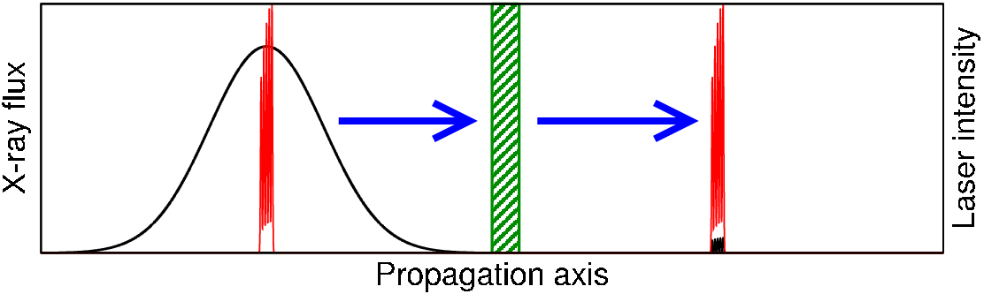
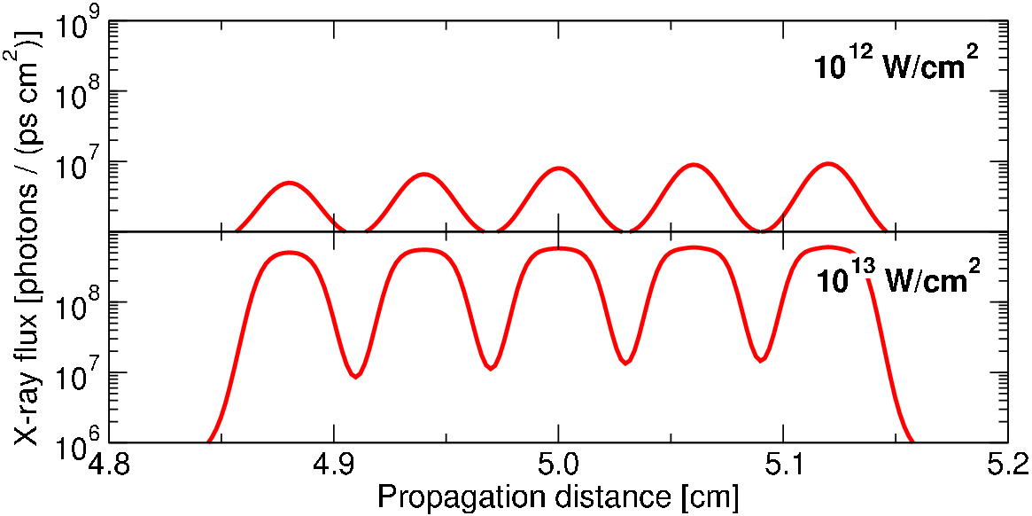
In Fig. 9, we demonstrate the principle of x-ray pulse shaping based on the effect electromagnetically induced transparency for x rays. On the left hand side of the gas cell, the initial laser and x-ray pulses are shown. The laser pulse has the shape of Eq. (41); the x-ray pulse has a Gaussian envelope (38). The pulses copropagate from left to right with the speed of light in vacuum $c$ through the gas cell which is filled with argon. Also in the cell the propagation speed deviates only minutely from $c$ (see the appendix). After passing through the cell—the right hand side of the figure—a pulse shape similar to the shape of the laser pulse is cut out of the broad x-ray pulse; the laser pulse remains unchanged. The fairly elaborate pulse shape (41) was imprinted approximately on the x-ray pulse. In Fig. 10, we show a close-up of the x-ray pulse on the right hand side of Fig. 9 for two different intensities of the dressing laser. We see a pronounced reduction of the initial peak x-ray flux $J_{\mathrm{X,0}}$ [Eq. (38)]. Due to the nonlinear dependence of the x-ray absorption cross section on the laser intensity (Fig. 4), the resulting transmitted pulse varies not only in the flux but also the general shape differs somewhat from the initial pulse. Overall the peak x-ray flux drops for $10^{13}\,{\rm{W/cm^{2}}}$ by a factor of 10. For neon, we found a stronger transmission on resonance which leads to a suppression of only a half for the same peak laser intensity [13].

Only the flux envelope of the x-ray pulse has been modified in Fig. 10. The time evolution of the phase of the x-ray pulses remains random. With the EIT for x rays method, the phase cannot be effectively manipulated because the magnitude of the polarizability and variation of the polarizability due to laser dressing are very small. Hence the magnitude and variation of the index of refraction of the gas is also very small. The x rays are basically fully absorbed before the phase can be influenced noticeably. This finding is in contrast to EIT for optical wavelengths where enormous changes of refraction and dispersion of the medium on the resonance can be observed and exploited see, e.g., Refs. 18, 19, 20, 21.

V Conclusion

In this paper, we investigated the complex index of refraction of atoms in the light of an intense optical laser in the x-ray region. This is a so-called two-color problem. The laser intensity is assumed to be sufficiently low such that the atoms are only dressed but not excited or ionized. We devised an ab initio theory to compute the basic atomic quantities, the dynamic dipole polarizability and the photoabsorption cross section, from which the real and imaginary part of the index of refraction, respectively, are determined. We describe the fundamental interaction of the atoms with the light in terms of quantum electrodynamics. The determination of the atomic properties involves resolvents. We use a single-vector Lanczos algorithm to compute the involved resolvents directly. The index of refraction is a concept of classical electrodynamics; it follows from the Maxwell equations. The transition from the quantum mechanics to classical physics is made by expressing the classical macroscopic polarizability in terms of quantum mechanical atomic polarizability and atomic absorption cross section. Finally, we consider a laser and an x-ray pulse copropagating through a gas cell using rate equations.

Our theory is applied to argon. We study the x-ray polarizability and absorption over a large range of dressing-laser intensities for parallel and perpendicular laser and x-ray polarization vectors. For parallel polarizations, we find electromagnetically induced transparency (EIT) for x rays on the Ar $\,1s\to 4p$ pre-edge resonance. The absorption is suppressed by a factor of $3.6$ when the laser is present. Also for perpendicular polarizations, the cross section on resonance shows a noticeable drop by a factor of $1.9$ for a laser intensity of $10^{13}\,{\rm{W/cm^{2}}}$ . As an application of EIT for x rays, the control of the absorption of the x rays allows one to imprint the shape of the laser pulse on x rays. We show the transmitted x-ray pulses for two different laser intensities which vary, apart from the flux, also due to the nonlinear dependence of the cross section on the laser intensity.

Our work opens up numerous possibilities for future research. The $K$ edge of argon is at $3205.9\,{\rm{eV}}$ [1] which implies a wavelength of the x rays of $3.9\,{\rm{\hbox{\AA}}}$ , i.e., our work opens up possibilities to shape hard x-ray pulses. Ultrashort, femtosecond, hard x-ray pulses come into reach. Especially, in conjunction with the emerging x-ray free electron lasers, our results may prove useful. The ability of pulse shaping x rays opens up possibilities for all-x-ray pump-probe experiments and quantum control of inner-shell processes.

Acknowledgements.

We thank Linda Young for fruitful discussions. C.B. was partly funded by a Feodor Lynen Research Fellowship from the Alexander von Humboldt Foundation. This work was supported by the Office of Basic Energy Sciences, Office of Science, U.S. Department of Energy, under Contract No. DE-AC02-06CH11357.

Appendix A Secondary physical processes

$\omega$ [ $\,{\rm{eV}}$ ]	$v_{\mathrm{p}}/c-1$	$v_{\mathrm{g}}/c-1$	$v_{\mathrm{p,pl}}/c-1$	$v_{\mathrm{g,pl}}/c-1$
0001.55	$-1.3\times 10^{-3}$	$-1.3\times 10^{-3}$	$1.4\times 10^{-8\phantom{0}}$	$-1.4\times 10^{-8\phantom{0}}$
3203.42	$\phantom{-}9.6\times 10^{-8}$	$\phantom{-}4.0\times 10^{-4}$	$3.4\times 10^{-15}$	$-3.4\times 10^{-15}$

Table 1: Estimate of the changes of the phase and group velocity due to secondary physical effects. We consider refraction and dispersion of the laser and the x rays by the argon-gas medium and the plasma for

I_{\mathrm{L,0}}=10^{13}\,{\rm{W/cm^{2}}}

Numerous secondary physical processes occur in course of the pulse propagation. The absorption of x rays leads to the production of ions and free electrons; in other words, a plasma. The ion production is governed by the rate equation

\Delta n^{\prime}_{\#}(z_{i})=n^{\prime}_{\#}(z_{i})\,\sigma^{\prime}(z_{i})\,J^{\prime}_{\mathrm{X}}(z_{i})\,\Delta t\;.

(42)

In the inner part of the gas cell the ion number density is constant; its maximum is $1.3\times 10^{13}\,{\rm{cm^{-3}}}$ . The ions which are created by photoionization have a $K$ vacancy. Each resonantly absorbed x ray generates a decay cascade which leads to the emission of $3.8$ electrons (Fig. 1(b) in Ref. 61).

The phase velocity [53] of laser and x-ray pulses in the medium is

v_{\mathrm{p}}(\omega)={c\over n(\omega)}

(43)

and their group velocity is [53, 21]:

v_{\mathrm{g}}(\omega)={c\over n(\omega)+\omega{\>\mathrm{d}n\over\>\mathrm{d}\omega}}\;,

(44)

where $n(\omega)$ denotes the real part of the refractive index in this appendix. We will show that both velocities differ only minutely from the corresponding velocities in vacuum for our choice of parameters.

The index of refraction of a plasma is

n_{\mathrm{pl}}(\omega)=\sqrt{1-{\omega_{\mathrm{p}}^{2}\over\omega^{2}}}\;,

(45)

with the plasma frequency $\omega_{\mathrm{p}}=\sqrt{4\pi\,n_{\mathrm{e}}}$ [53]. The group velocity for a plasma is

v_{\mathrm{g,pl}}(\omega)=c\,n_{\mathrm{pl}}(\omega)\;.

(46)

The refractive index of argon gas for laser light is obtained from Eq. (37). We use the dynamic polarizability of argon atoms for $\omega_{\mathrm{L}}=1.55\,{\rm{eV}}$ [62, 63] which is $11.42\,e^{2}\,a_{0}^{2}\,{\rm{E_{\mathit{h}}}}^{-1}$ . The real part of the refractive index follows with Eq. (37) to $n(1.55\,{\rm{eV}})=1.0013$ for the physical parameters from Sec. III.

The group velocity of x rays in argon gas follows from Eq. (44). We insert the derivative of the index of refraction letting $\mu=0$ in Eq. (37) yielding

v_{\mathrm{g,X}}(\omega_{\mathrm{X}})={c\over 1+2\pi\,n_{\#}\,[\alpha_{\mathrm{I}}(\omega_{\mathrm{X}})+\omega_{\mathrm{X}}\,{\>\mathrm{d}\alpha_{\mathrm{I}}\over\>\mathrm{d}\omega}(\omega_{\mathrm{X}})]}\;.

(47)

The polarizability of argon on resonance is taken from the curve in Fig. 5 and its numerical derivative. The group velocity of the laser in argon gas $v_{\mathrm{g,L}}(\omega_{\mathrm{L}})$ is obtained from Eq. (47)—with “X” replaced by “L”—by inserting the slope of the line used for the linear interpolation of the dynamic polarizability [62, 63].

In Table 1, we list exemplary estimates of the secondary physical effects. We assume a laser intensity of $10^{13}\,{\rm{W/cm^{2}}}$ . Overall we observe that these effects are very small under the conditions of this paper. However, for increasing gas densities and/or increasing laser intensities, these factors become relevant and have to be accounted for. The largest difference to $c$ occurs for the phase and group velocities of the laser in the argon gas. We observe that the maximum of the phase velocities and the group velocities are essentially the same. This is unlike EIT for optical wavelengths where the group velocity and phase velocity on resonance differ largely, leading to slow light [18, 21]. For lower laser intensities, the plasma related velocities, $v_{\mathrm{p,pl}}$ and $v_{\mathrm{g,pl}}$ increase slightly because a larger fraction of the x-ray pulse is absorbed leading to a denser plasma. Conversely, these velocities are smaller for higher laser intensities as long as the laser intensity remains far below the saturation intensity. As soon as the laser begins to contribute to the plasma formation, $v_{\mathrm{p,pl}}$ and $v_{\mathrm{g,pl}}$ deviate noticeably from $c$ .

References

[1] A. C. Thompson, D. T. Attwood, E. M. Gullikson, M. R. Howells, J. B. Kortright, A. L. Robinson, J. H. Underwood, K.-J. Kim, J. Kirz, I. Lindau, et al., X-ray data booklet (Lawrence Berkeley National Laboratory, Berkeley, 2001), 2nd ed.
[2] F. J. Wuilleumier and M. Meyer, J. Phys. B 39, R425 (2006).
[3] L. Young, D. A. Arms, E. M. Dufresne, R. W. Dunford, D. L. Ederer, C. Höhr, E. P. Kanter, B. Krässig, E. C. Landahl, E. R. Peterson, et al., Phys. Rev. Lett. 97, 083601 (2006).
[4] R. Santra, R. W. Dunford, and L. Young, Phys. Rev. A 74, 043403 (2006).
[5] Z.-H. Loh, M. Khalil, R. E. Correa, R. Santra, C. Buth, and S. R. Leone, Phys. Rev. Lett. 98, 143601 (2007), arXiv:physics/0703149.
[6] R. Santra, C. Buth, E. R. Peterson, R. W. Dunford, E. P. Kanter, B. Krässig, S. H. Southworth, and L. Young, J. Phys.: Conf. Ser. 88, 012052 (2007), arXiv:0712.2556.
[7] E. Gagnon, P. Ranitovic, X.-M. Tong, C. L. Cocke, M. M. Murnane, H. C. Kapteyn, and A. S. Sandhu, Science 317, 1374 (2007).
[8] C. Buth and R. Santra, Phys. Rev. A 77, 013413 (2008a), arXiv:0711.3203.
[9] E. R. Peterson, C. Buth, D. A. Arms, R. W. Dunford, E. P. Kanter, B. Krässig, E. C. Landahl, S. T. Pratt, R. Santra, S. H. Southworth, et al., Appl. Phys. Lett. 92, 094106 (2008), arXiv:0802.1894.
[10] C. Buth and R. Santra, J. Chem. Phys. 129, 134312 (2008b), arXiv:0809.0146.
[11] L. Young, C. Buth, R. W. Dunford, P. J. Ho, E. P. Kanter, B. Krässig, E. R. Peterson, N. Rohringer, R. Santra, and S. H. Southworth, Rev. Mex. Fís. (2008), manuscript submitted, arXiv:0809.3537.
[12] C. Buth and R. Santra, Phys. Rev. A 75, 033412 (2007), arXiv:physics/0611122.
[13] C. Buth, R. Santra, and L. Young, Phys. Rev. Lett. 98, 253001 (2007), arXiv:0705.3615.
[14] C. Buth, R. Santra, and L. Young, Rev. Mex. Fís. (2008), manuscript submitted, arXiv:0805.2619.
[15] S. E. Harris, J. E. Field, and A. Imamoǧlu, Phys. Rev. Lett. 64, 1107 (1990).
[16] K.-J. Boller, A. Imamoǧlu, and S. E. Harris, Phys. Rev. Lett. 66, 2593 (1991).
[17] S. E. Harris, Phys. Today 50, 36 (1997).
[18] L. V. Hau, S. E. Harris, Z. Dutton, and C. H. Behroozi, Nature 397, 594 (1999).
[19] D. F. Phillips, A. Fleischhauer, A. Mair, R. L. Walsworth, and M. D. Lukin, Phys. Rev. Lett. 86, 783 (2001).
[20] M. Lukin and A. Imamoǧlu, Nature 413, 273 (2001).
[21] M. Fleischhauer, A. Imamoǧlu, and J. P. Marangos, Rev. Mod. Phys. 77, 633 (2005).
[22] R. Santra, E. Arimondo, T. Ido, C. H. Greene, and J. Ye, Phys. Rev. Lett. 94, 173002 (2005).
[23] M. O. Krause and J. H. Oliver, J. Phys. Chem. Ref. Data 8, 329 (1979).
[24] M. H. Chen, B. Crasemann, and H. Mark, Phys. Rev. A 21, 436 (1980).
[25] V. Schmidt, Electron spectrometry of atoms using synchrotron radiation (Cambridge University Press, Cambridge, 1997), ISBN 0-521-55053-X.
[26] A. M. Weiner, Rev. Sci. Instrum. 71, 1929 (2000).
[27] M. Borland, Phys. Rev. ST Accel. Beams 8, 074001 (2005).
[28] A. Szabo and N. S. Ostlund, Modern quantum chemistry: Introduction to advanced electronic structure theory (McGraw-Hill, New York, 1989), 1st, revised ed., ISBN 0-486-69186-1.
[29] E. Merzbacher, Quantum mechanics (John Wiley & Sons, New York, 1998), 3rd ed., ISBN 0-471-88702-1.
[30] We assume that the continuum of core-excited states is discretized. In Sec. II.3 we introduce a complex absorbing potential and a basis set to accomplish this.
[31] D. P. Craig and T. Thirunamachandran, Molecular quantum electrodynamics (Academic Press, London, 1984), ISBN 0-486-40214-2.
[32] Equation (4) was obtained by converting the equation from SI units to atomic units. Therefore factors $\alpha$ , the fine-structure constant, are missing which are typically found when converting equations from Gaussian units to atomic units.
[33] M. O. Scully and M. S. Zubairy, Quantum optics (Cambridge University Press, Cambridge, New York, Melbourne, 1997), ISBN 0-521-43595-1.
[34] V. I. Kukulin, V. M. Krasnopol’sky, and J. Horáček, Theory of resonances (Kluwer, Dordrecht, 1989), ISBN 90-277-2364-8.
[35] N. Moiseyev, Phys. Rep. 302, 211 (1998a).
[36] R. Santra and L. S. Cederbaum, Phys. Rep. 368, 1 (2002).
[37] C. Buth, R. Santra, and L. S. Cederbaum, Phys. Rev. A 69, 032505 (2004), arXiv:physics/0401081.
[38] A. J. F. Siegert, Phys. Rev. 56, 750 (1939).
[39] J. J. Sakurai, Modern quantum mechanics (Addison-Wesley, Reading (Massachusetts), 1994), 2nd ed., ISBN 0-201-53929-2.
[40] N. B. Delone and V. P. Krainov, Physics – Uspekhi 42, 669 (1999).
[41] P. Meystre and M. Sargent III, Elements of quantum optics (Springer, Berlin, 1991), 2nd ed., ISBN 3-540-54190-X.
[42] J. C. Slater, Phys. Rev. 81, 385 (1951).
[43] J. C. Slater and K. H. Johnson, Phys. Rev. B 5, 844 (1972).
[44] We restrict ourselves to single core holes due to only moderate x-ray intensities.
[45] N. Moiseyev, J. Phys. B 31, 1431 (1998b).
[46] U. V. Riss and H.-D. Meyer, J. Phys. B 31, 2279 (1998).
[47] H. O. Karlsson, J. Chem. Phys. 109, 9366 (1998).
[48] J. Als-Nielsen and D. McMorrow, Elements of modern x-ray physics (John Wiley & Sons, New York, 2001), ISBN 0-471-49858-0.
[49] C. Lanczos, J. Res. Natl. Bur. Stand. 45, 255 (1950).
[50] J. K. Cullum and R. A. Willoughby, Lanczos algorithms for large symmetric eigenvalue computations (Birkhäuser, Boston, 1985), ISBN 0-8176-3292-6-F, 3-7643-3292-6-F, two volumes.
[51] H.-D. Meyer and S. Pal, J. Chem. Phys. 91, 6195 (1989).
[52] T. Sommerfeld, U. V. Riss, H.-D. Meyer, L. S. Cederbaum, B. Engels, and H. U. Suter, J. Phys. B 31, 4107 (1998).
[53] J. D. Jackson, Classical electrodynamics (John Wiley & Sons, Chichester, New York, 1998), 3rd ed., ISBN 0-471-30932-X.
[54] C. Buth and R. Santra, fella – the free electron laser atomic, molecular, and optical physics program package, Argonne National Laboratory, Argonne, Illinois, USA (2008c), version 1.3.0, with contributions by Mark Baertschy, Kevin Christ, Chris H. Greene, Hans-Dieter Meyer, and Thomas Sommerfeld, www.cse.anl.gov/Fundamental_Interactions/FELLA_main.shtml.
[55] F. Herman and S. Skillman, Atomic structure calculations (Prentice-Hall, Englewood Cliffs, NJ, 1963).
[56] J. L. Campbell and T. Papp, At. Data Nucl. Data Tables 77, 1 (2001).
[57] S. Augst, D. Strickland, D. D. Meyerhofer, S. L. Chin, and J. H. Eberly, Phys. Rev. Lett. 63, 2212 (1989).
[58] G. Liggett and J. S. Levinger, J. Opt. Soc. Am. 58, 109 (1968).
[59] A. E. Kingston, J. Opt. Soc. Am. 54, 1145 (1964).
[60] The temperature and pressure of the argon gas, for which the refractive index is determined, are not stated in Ref. 58. Yet in Ref. 58, the authors refer to a similar study by Kingston [59] who gives results for normal temperature and pressure (NTP), i.e., $20\,{}^{\circ}\mathrm{C}$ and $1\,{\rm{atm}}$ . Hence, to compare with Liggett and Levinger, we assume NTP for argon gas.
[61] J. Doppelfeld, N. Anders, B. Esser, F. von Busch, H. Scherer, and S. Zinz, J. Phys. B 26, 445 (1993).
[62] N. K. Rahman, A. Rizzo, and D. L. Yeager, Chem. Phys. Lett. 166, 565 (1990).
[63] The value of $\omega_{\mathrm{L}}=1.55\,{\rm{eV}}=0.057\,{\rm{E_{\mathit{h}}}}$ is determined by linear interpolation between the points $0.05\,{\rm{E_{\mathit{h}}}}$ and $0.1\,{\rm{E_{\mathit{h}}}}$ from Ref. 62.

58, 59