Classifying smooth lattice polytopes
via toric fibrationsThanks: AD was partially supported by UBACYT X042 and X064, CONICET PIP 5617 and ANPCyT PICT 20569, Argentina.Thanks: SDR was partially supported by Vetenskapsrådet’s grant NT:2006-3539, and the CIAM (Center of industrial and applied mathematics).

Alicia Dickenstein, Sandra Di Rocco, Ragni Piene Address: Departamento de Matemática, FCEN, Universidad de Buenos Aires, Ciudad Universitaria - Pab. I, (1428) Buenos Aires, Argentina Email address: alidick@dm.uba.ar Address: Department of Mathematics, KTH, SE-10044 Stockholm, Sweden Email address: dirocco@math.kth.se Address: CMA/Department of Mathematics, University of Oslo, P. O. Box 1053 Blindern, NO-0316 Oslo, Norway Email address: ragnip@math.uio.no

Date: August 24, 2026

Abstract.

We show that any smooth ${\mathbb{Q}}$ -normal lattice polytope $P$ of dimension $n$ and degree $d$ is a strict Cayley polytope if $n\geq 2d+1$ . This gives a sharp answer, for this class of polytopes, to a question raised by V. V. Batyrev and B. Nill.

1. Introduction

Let $P$ be an $n$ -dimensional lattice polytope (i.e., a convex polytope with integer vertices) in ${\mathbb{R}}^{n}$ . We represent it as an intersection of half spaces

P\,=\,\cap_{i=1}^{r}H_{\rho_{i},-a_{i}}^{+},

where $H_{\rho_{i},-a_{i}}^{+}=\{x\in{\mathbb{R}}^{n}\,|\,\langle\rho_{i},x\rangle\geq-a_{i}\}$ are the half spaces, $H_{\rho_{i},-a_{i}}=\{x\in{\mathbb{R}}^{n}\,|\,\langle\rho_{i},x\rangle=-a_{i}\}$ the supporting hyperplanes, $\rho_{i}$ the corresponding primitive inner normals, and $a_{i}\in{\mathbb{Z}},\,i=1,\dots,r$ . Recall that an $n$ -dimensional lattice polytope $P$ is smooth if every vertex is equal to the intersection of $n$ of the hyperplanes $H_{\rho_{i},-a_{i}}$ , and if the corresponding $n$ normal vectors $\rho_{i}$ form a lattice basis for ${\mathbb{Z}}^{n}\subset{\mathbb{R}}^{n}$ . Smooth polytopes are sometimes called Delzant polytopes or regular polytopes.

Definition 1.1.

Let $P=\cap_{i=1}^{r}H_{\rho_{i},-a_{i}}^{+}\subset{\mathbb{R}}^{n}$ be an $n$ -dimensional lattice polytope. Define $P^{(s)}:=\cap_{i=1}^{r}H_{\rho_{i},-a_{i}+s}^{+},$ for $s\geq 1$ .

Note that the lattice points of $P^{(1)}$ are precisely the interior lattice points of $P$ .

Definition 1.2.

Let $P$ be a smooth $n$ -dimensional lattice polytope and $s\geq 1$ an integer. Let $m$ be a vertex of $P$ . Reorder the hyperplanes so that $\{m\}=\cap_{i=1}^{n}H_{\rho_{i},-a_{i}}$ . We say that $P$ is $s$ -spanned at $m$ if the lattice point $m(s)$ , defined by $\{m(s)\}=\cap_{i=1}^{n}H_{\rho_{i},-a_{i}+s}$ , lies in $P^{(s)}$ . We say that $P$ is $s$ -spanned if $P$ is $s$ -spanned at every vertex.

If $\{m\}=\cap_{1}^{n}H_{\rho_{i},-a_{i}}$ , we can write $m=(-a_{1},\ldots,-a_{n})$ in the dual basis of $\rho_{1},\ldots,\rho_{n}$ , and similarly $m(s)=(-a_{1}+s,\ldots,-a_{n}+s)$ . It follows from the definition that if $P$ is $s$ -spanned, then $P^{(s)}\cap{\mathbb{Z}}^{n}\neq\emptyset$ .

Example 1.3.

Let $P$ be the smooth polytope obtained from the simplex $d\Delta_{3}$ by removing the simplex $\Delta_{3}=\Conv\{(0:0:0),(1:0:0),(0:1:0),(0:0:1)\}$ , see Figure 1. Assume $d\geq 4$ . Then $P^{(1)}\neq\emptyset$ , but $P$ is not $1$ -spanned. In fact, consider the vertex $m$ of $P$ , given by $\{m\}=\{(1:0:0)\}=(y=0)\cap(z=0)\cap(x+y+z=1)$ , then the lattice point $m(1)$ , given by $\{m(1)\}=\{(0:1:1)\}=(y=1)\cap(z=1)\cap(x+y+z=2)$ , is not a point in $P^{(1)}$ . Similarly for the vertices $(0:1:0)$ and $(0:0:1)$ .

Note that if we instead remove $2\Delta_{3}$ , then the resulting polytope is $1$ -spanned. In this case, the vertices $(2:0:0)$ , $(0:2:0)$ , and $(0:0:2)$ all “go” to the same lattice point $(1:1:1)$ , which is an interior point of the polytope.

Figure 1.

We recall the definitions of degree and codegree of a lattice polytope introduced in [1].

Definition 1.4.

Let $P\subset{\mathbb{R}}^{n}$ be an $n$ -dimensional lattice polytope. The codegree of $P$ is the natural number

\textstyle\codeg(P):=\min_{{\mathbb{N}}}\{k\,|\,(kP)^{(1)}\cap{\mathbb{Z}}^{n}\neq\emptyset\}.

The degree of $P$ is

\deg(P):=n+1-\codeg(P).

We further introduce a more “refined” notion of codegree.

Definition 1.5.

Let $P\subset{\mathbb{R}}^{n}$ be an $n$ -dimensional lattice polytope. The ${\mathbb{Q}}$ -codegree of $P$ is defined as

\textstyle\codeg_{\mathbb{Q}}(P):=\inf_{{\mathbb{Q}}}\{\frac{a}{b}\,|\,(aP)^{(b)}\neq\emptyset\}.

The number $\codeg_{\mathbb{Q}}(P)$ is well defined, since $m(aP^{(b)})=(maP)^{(mb)}$ and, for any polytope $P^{\prime}$ , we have $P^{\prime}\neq\emptyset$ if and only if $mP^{\prime}\neq\emptyset$ for every integer $m\geq 1$ . Moreover, it is clear that ${\codeg_{\mathbb{Q}}(P)}\leq\codeg(P)$ holds.

Example 1.6.

Let $\Delta_{n}$ denote the $n$ -dimensional simplex. Then we have $\codeg_{{\mathbb{Q}}}(2\Delta_{n})=\frac{n+1}{2}$ and $\codeg(2\Delta_{n})=\lceil{\frac{n+1}{2}}\rceil$ .

As we shall see in Proposition 2.2, the following definition embodies the polytope version of the notion of nef value for projective varieties.

Definition 1.7.

Let $P\subset{\mathbb{R}}^{n}$ be an $n$ -dimensional smooth lattice polytope. The nef value of $P$ is

\textstyle\tau(P)=\inf_{\mathbb{Q}}\{\frac{a}{b}\,|\,aP\text{ is $b$-spanned}\}.

Remark 1.8.

Clearly, the inequality $\tau(P)\geq\codeg_{\mathbb{Q}}(P)$ always holds. It can be strict, as in Example 1.3, where $\codeg(P)=\codeg_{\mathbb{Q}}(P)=1$ and $\tau(P)=2$ .

Observe also that when $\tau(P)$ is an integer, it follows from Lemma 2.4 below that $\tau(P)\geq\codeg(P)$ .

Definition 1.9.

An $n$ -dimensional lattice polytope $P$ in ${\mathbb{R}}^{n}$ is called ${\mathbb{Q}}$ -normal if $\codeg_{\mathbb{Q}}(P)=\tau(P)$ .

We shall now explain the notion of generalized Cayley polytopes — these are particular examples of the twisted Cayley polytopes defined in [5].

Definition 1.10.

Let $P_{0},\ldots,P_{k}\subset{\mathbb{R}}^{m}$ be lattice polytopes in ${\mathbb{Z}}^{m}$ , $e_{1},\ldots,e_{k}$ a basis for ${\mathbb{Z}}^{k}$ and $e_{0}=0\in{\mathbb{Z}}^{k}$ . If $\{m_{i}^{j}\}_{i}$ are the vertices of $P_{j}$ , so that $P_{j}={\rm Conv}\{m_{i}^{j}\}$ is the convex hull, and $s$ is a positive integer, consider the polytope ${\rm Conv}\{(m_{i}^{j},se_{j})\}_{i,j}\subseteq{\mathbb{R}}^{m+k}$ . Any polytope $P$ which is affinely equivalent to this polytope will be called an $s$ th order generalized Cayley polytope associated to $P_{0},\ldots,P_{k}$ , and it will be denoted by

P\cong[P_{0}\ast P_{1}\ast\cdots\ast P_{k}]^{s}.

If all the polytopes $P_{0},\dots,P_{k}$ have the same normal fan $\Sigma$ (equivalently, if they are strictly combinatorially equivalent), we call $P$ strict, and denote it by

P\cong\Cayley^{s}_{\Sigma}(P_{0},\ldots,P_{k}).

If in addition $s=1$ , we write $P\cong\Cayley_{\Sigma}(P_{0},\ldots,P_{k})$ and call $P$ a strict Cayley polytope.

Smooth generalized strict Cayley polytopes are natural examples of ${\mathbb{Q}}$ -normal polytopes. In Proposition 3.9 we give sufficient conditions for $P\cong\Cayley^{s}_{\Sigma}(P_{0},\ldots,P_{k})$ to be ${\mathbb{Q}}$ -normal, and we compute the common value $\codeg_{\mathbb{Q}}(P)=\tau(P)$ in this case.

In [1] Batyrev and Nill posed the following question:

Question. Given an integer $d$ , does there exist an integer $N(d)$ such that every lattice polytope of degree $d$ and dimension $\geq N(d)$ is a Cayley polytope?

A first general answer was given by C. Haase, B. Nill, and S. Payne in [10], where they prove the existence of a lower bound which is quadratic in $d$ .

In this article we give an optimal linear bound in the case of smooth ${\mathbb{Q}}$ -normal lattice polytopes, and show that polytopes of dimension greater than or equal to this bound are strict Cayley polytopes.

Answer. For $n$ -dimensional smooth ${\mathbb{Q}}$ -normal lattice polytope, we can take $N(d)=2d+1$ . More precisely, if $P$ is a smooth ${\mathbb{Q}}$ -normal lattice polytope of dimension $n$ and degree $d$ such that $n\geq 2d+1$ , then $P$ is a strict Cayley polytope.

Observe that the condition $n\geq 2\deg(P)+1$ is equivalent to $\codeg(P)\geq\frac{n+3}{2}$ . Furthermore, note that our bound is sharp: consider the standard $n$ -dimensional simplex $\Delta_{n}$ and let $P:=2\Delta_{n}$ as in Example 1.6. Then, $\tau(P)=\codeg_{\mathbb{Q}}(P)=\frac{n+1}{2}=\frac{n+3}{2}-1$ and $P$ is not a Cayley polytope. It is, however, a generalized Cayley polytope, with $s=2$ . We conjecture that an even smaller linear bound, like $\frac{n+1}{s}$ , should suffice for the polytope to be an $s$ -th order generalized Cayley polytope.

We shall deduce our answer from Theorem 1.12 below, which gives a characterization of ${\mathbb{Q}}$ -normal smooth lattice polytopes with big codegree. Before stating our main theorem, we recall the notion of a defective projective variety.

Definition 1.11.

Let $X\subset{\mathbb{P}}^{N}$ be a projective variety over an algebraically closed field and denote by $X^{*}\subset({\mathbb{P}}^{N})^{\vee}$ its dual variety in the dual projective space. Then $X$ is defective if $X^{*}$ is not a hypersurface, and its defect is the natural number $\delta=N-1-\dim(X^{*})$ .

Theorem 1.12.

Let $P\subset{\mathbb{R}}^{n}$ be a smooth lattice polytope of dimension $n$ . Then the following statements are equivalent:

(1)

$P$ is ${\mathbb{Q}}$ -normal and $\codeg(P)\geq\frac{n+3}{2}$ ,
(2)

$P=\Cayley_{\Sigma}(P_{0},\ldots,P_{k})$ is a smooth strict Cayley polytope, where $k+1=\codeg(P)$ and $k>\frac{n}{2}$ ,
(3)

the (complex) toric polarized variety $(X,L)$ corresponding to $P$ is defective, with defect $\delta=2\codeg(P)-2-n$ .

We conjecture that the assumption $\tau(P)=\codeg_{\mathbb{Q}}(P)$ always holds for smooth lattice polytopes satisfying $\codeg(P)\geq\frac{n+3}{2},$ and we therefore expect that the above classification holds for all smooth polytopes.

Our proof of Theorem 1.12 relies on the study of the nef value of nonsingular toric polarized varieties. This is developed in Section 2. Section 3 contains the study of generalized Cayley polytopes in terms of fibrations. In particular, for smooth generalized strict Cayley polytopes $P^{s}=\Cayley_{\Sigma}^{s}(P_{0},\ldots,P_{k})$ such that $s<k+1$ and $\dim P_{i}+1<\frac{k+1}{s}$ for all $i$ , Proposition 3.9 shows that $\codeg(P^{s})>1$ , providing a family of lattice polytopes without interior lattice points. Section 4 contains the proof of the classification Theorem 1.12, together with some final comments.

2. The codegree and the nef value

Let $X$ be a nonsingular projective variety over an algebraically closed field, and let $L$ be an ample line bundle (or divisor) on $X$ .

Definition 2.1.

Assume that the canonical divisor $K_{X}$ is not nef. The nef value of $(X,L)$ is defined as

\textstyle\tau_{L}:=\min_{\mathbb{R}}\{t\,|\,K_{X}+tL\text{ is nef}\}.

By Kawamata’s rationality theorem [9, Prop. 3.1, p. 619], the nef value $\tau_{L}$ is a positive rational number.

Proposition 2.2.

Let $X$ be a nonsingular projective toric variety of dimension $n$ , and let $L$ be an ample line bundle on $X$ . Let $P\subset{\mathbb{R}}^{n}$ be the associated $n$ -dimensional smooth lattice polytope. Then

\tau_{L}=\tau(P).

Proof.

If we write the polytope $P$ as $\cap_{i=1}^{r}H^{+}_{\rho_{i},-a_{i}}$ , then $L=\sum_{i=1}^{r}a_{i}D_{i}$ , where the $D_{i}$ are the invariant divisors on $X$ . Since $K_{X}=-\sum_{i=1}^{r}D_{i}$ , the polytope associated to $X$ and the adjoint line bundle $bK_{X}+aL$ is

\textstyle P_{bK_{X}+aL}=\cap_{i=1}^{r}H^{+}_{\rho_{i},-a\cdot a_{i}+b}=(aP)^{(b)}.

The lattice points of $(aP)^{(b)}$ form a basis for the vector space of global sections of $bK_{X}+aL$ ,

H^{0}(X,bK_{X}+aL)=\oplus_{m\in(aP)^{(b)}\cap M}{\mathbb{C}}\chi^{m}

(see [13, Lemma 2.3, p. 72]).

Denote by $\Sigma$ the fan of $X$ , let $x(\sigma)$ be the fixed point associated to the $n$ -dimensional cone $\sigma=\langle\rho_{1},\ldots,\rho_{n}\rangle\in\Sigma$ , and let $U_{\sigma}=X\setminus(\cup_{\tau\not\subset\sigma}V(\tau))$ be the affine patch containing $x(\sigma)$ . The restriction of a generator $\chi^{m}\in H^{0}(X,bK_{X}+aL)$ to $U_{\sigma}$ is

\chi^{m}|_{U_{\sigma}}=\Pi_{1}^{n}\chi_{i}^{\langle m,\rho_{i}\rangle-(-a\cdot a_{i}+b)},

where $\chi_{1},\ldots,\chi_{n}$ is a system of local coordinates such that $x(\sigma)=(0,\ldots,0).$ It follows that the line bundle $bK_{X}+aL$ is spanned, or globally generated, at $x(\sigma)$ (i.e., it has at least one nonvanishing section at $x(\sigma)$ ) if and only if the lattice point $(-a\cdot a_{1}+b,\ldots,-a\cdot a_{n}+b)$ , written with respect to the dual basis of $\rho_{1},\ldots,\rho_{n}$ , is in $(aP)^{(b)}$ .

Because the base locus of a line bundle is invariant under the torus action, if it is non empty, it must be the union of invariant subspaces. Hence it has to contain fixed points. It follows that $bK_{X}+aL$ is spanned if and only if it is spanned at each fixed point, hence if and only if the polytope $aP$ is $b$ -spanned. ∎

Corollary 2.3.

Let $P\subset{\mathbb{R}}^{n}$ be an $n$ -dimensional smooth lattice polytope. Then

(1)

$\codeg(P)=\codeg_{\mathbb{Q}}(P)=\tau(P)=n+1$ if and only if $P=\Delta_{n}.$
(2)

If $P\neq\Delta_{n},$ then $\codeg_{\mathbb{Q}}(P)\leq\tau(P)\leq n.$

Proof.

Let $(X,L)$ be the polarized nonsingular toric variety corresponding to $P$ . In [12, Cor. 4.2] it is proven that $K_{X}+H$ is spanned for any line bundle $H$ on $X$ such that $H\cdot C\geq n$ for all invariant curves $C$ on $X$ , unless $X={\mathbb{P}}^{n}$ and $H={\cal O}_{{\mathbb{P}}^{n}}(n).$

Because the line bundle $L$ is ample, we have $L\cdot C\geq 1$ and thus $nL\cdot C\geq n$ , for all invariant curves $C$ . It follows that if $X\neq{\mathbb{P}}^{n}$ or $nL\neq{\cal O}_{{\mathbb{P}}^{n}}(n)$ , then $\tau_{L}=\tau(P)\leq n$ . This proves $(2)$ . If $(X,L)=({\mathbb{P}}^{n},{\cal O}_{{\mathbb{P}}^{n}}(1))$ , then $\tau_{L}=\tau(P)=n+1$ , because $K_{{\mathbb{P}}^{n}}={\cal O}_{{\mathbb{P}}^{n}}(-n-1)$ . The corresponding polytope is $P=\Delta_{n}$ and $\codeg(P)=\codeg_{\mathbb{Q}}(P)=\tau(P)=n+1$ , as stated in $(1)$ . ∎

Lemma 2.4.

Let $P\subset{\mathbb{R}}^{n}$ be a smooth $n$ -dimensional polytope with codegree $c$ and nef value $\tau$ . Then $\tau\in{\mathbb{Q}}_{>0}$ and $\tau>c-1$ .

Proof.

Let $(X,L)$ be the polarized projective toric variety associated to $P$ . Then $\tau=\tau_{L}\in{{\mathbb{Q}}}_{>0}$ . By [2, Lemma 0.8.3] $K_{X}+\tau L$ is nef (and not ample). For any $s\geq\tau$ , $K_{X}+sL=(K_{X}+\tau L)+(s-\tau)L$ is also nef. When $s$ is an integer, this implies that $K_{X}+sL$ is spanned, hence $(sP)^{(1)}\cap{\mathbb{Z}}^{n}\neq\emptyset$ . Taking $s=c-1$ and observing that $((c-1)P)^{(1)}$ has no lattice points, we deduce that $c-1<\tau$ , as claimed. ∎

Let $\tau(P)=\frac{a}{b},$ where $a,b$ are coprime. On complete toric varieties, nef line bundles with integer coefficients are spanned (see [12, Thm. 3.1]). It follows that the linear system $|bK_{X}+aL|$ defines a morphism

\varphi:X\to{\mathbb{P}}^{N},

where $N=|(aP)^{(b)}\cap{\mathbb{Z}}^{n}|-1$ . The Remmert–Stein factorization gives $\varphi=f\circ\varphi_{P},$ where $\varphi_{P}:X\to Y$ is a morphism with connected fibers onto a normal toric variety $Y$ such that $\dim Y=\dim(aP)^{(b)}$ and $f:Y\to{\mathbb{P}}^{N}$ . Moreover, $\varphi_{P}$ is the contraction of a face of the nef cone NE( $X$ ) [3, Lemma 4.2.13, p. 94].

Remark 2.5.

If the morphism $\varphi_{P}$ contracts a line, i.e., if there is a curve $C$ such that $L\cdot C=1$ and $\varphi_{P}(C)$ is a point, then $\tau(P)$ is necessarily an integer. In fact $0=(bK_{X}+aL)\cdot C$ implies $\frac{a}{b}=-K_{X}\cdot C\in{\mathbb{Z}}$ .

Lemma 2.6.

Let $P$ be a smooth $n$ -dimensional polytope and let $(X,L)$ be the corresponding polarized toric variety. If $\tau(P)>\frac{n+1}{2}$ , then there exists an invariant line on $X$ contracted by the nef value morphism $\varphi_{P}$ . In particular, $\tau(P)\in{\mathbb{Z}}$ , and $\tau(P)\geq\codeg(P)$ . If, moreover, $\varphi_{P}$ is not birational, then $\varphi_{P}$ is the contraction of an extremal ray in the nef cone, unless $n$ is even and $P=\Delta_{\frac{n}{2}}\times\Delta_{\frac{n}{2}}$ .

Proof.

Because the nef value morphism is the contraction of a face of the Mori cone, it contracts at least one extremal ray. Take $C$ to be a generator of this ray. Recall that, by Mori’s Cone theorem (see e.g. [6, p. 25]), $n+1\geq-K_{X}\cdot C$ . Because $(K_{X}+\tau(P)L)\cdot C=0$ , we have

\textstyle n+1\geq-K_{X}\cdot C=\tau(P)L\cdot C>\frac{n+1}{2}L\cdot C,

which gives $L\cdot C=1$ and $\tau(P)=-K_{X}\cdot C\in{\mathbb{Z}}$ . Lemma 2.4 gives $\tau(P)>\codeg(P)-1$ from which we deduce that $\tau(P)\geq\codeg(P)$ . If $\varphi_{P}$ is not birational, the last assertion follows from [4, (3.1.1.1), p. 30]. ∎

We will also need the following key lemma. This lemma, and its proof, is essentially the same as [3, Lemma 7.1.6, p. 157].

Lemma 2.7.

Let $(X,L)$ be the polarized nonsingular toric variety associated to a smooth ${\mathbb{Q}}$ -normal lattice polytope $P$ . Then the morphism $\varphi_{P}$ is not birational.

Proof.

Let $\frac{a}{b}=\tau(P).$ Assume the morphism $\varphi_{P}$ is birational. By [3, Lemma 2.5.5, p. 60] there is an integer $m$ and an effective divisor $D$ on $X$ such that

m(bK_{X}+aL)=L+D.

It follows that $D\in|mbK_{X}+(ma-1)L|$ , and thus $\codeg_{\mathbb{Q}}(P)\leq\frac{ma-1}{mb}<\frac{a}{b}=\tau(P)$ , which contradicts the assumption that $P$ is ${\mathbb{Q}}$ -normal. ∎

3. Generalized Cayley Polytopes and toric fibrations

Strict generalized Cayley polytopes (recall Definition 1.10) correspond to particularly nice toric fibrations, namely projective bundles. We will compute their associated nef values and codegrees. We refer to [5, Section 3] for further details on toric fibrations.

Definition 3.1.

A polarized toric fibration is a quintuple $(f,X,Y,F,L),$ where

(1)

$X$ and $Y$ are normal toric varieties with $\dim(Y)<\dim(X)$ ,
(2)

$f\colon X\to Y$ is an equivariant flat surjective morphism with connected fibers,
(3)

the general fiber of $f$ is isomorphic to the (necessarily toric) variety $F$ ,
(4)

$L$ is an ample line bundle on $X$ .

There is a $1$ - $1$ correspondence between polarized toric fibrations and fibrations of polytopes, making Definition 3.1 equivalent to the following.

Definition 3.2.

Let $\pi:M\to\Lambda$ be a surjective map of lattices and let $P_{0},\ldots,P_{k}\subset M_{\mathbb{R}}$ be lattice polytopes. We call $\pi$ a fibration with fiber $\Delta$ if

(1)

$\pi_{\mathbb{R}}(P_{i})=m_{i}\in\Lambda$ for every $i=0,\ldots,k$ ,
(2)

$m_{0},\ldots,m_{k}$ are all distinct and are the vertices of

$\Delta:=\Conv\{m_{0},\ldots,m_{k}\}\subset\Lambda_{{\mathbb{R}}},$
(3)

$P_{0},\ldots,P_{k}$ have the same normal fan, $\Sigma$ .

In [5, Lemma 3.6] it is proven that $(f,X,Y,F,L)$ is a toric fibration if and only if the polytope $P\subset M_{\mathbb{R}}$ associated to $(X,L)$ has the structure of a fibration. More precisely, $(f,X,Y,F,L)$ is a toric fibration if and only if there is a sublattice $\Lambda^{\vee}\hookrightarrow M^{\vee}$ such that the dual map $\pi:M\to\Lambda$ is a fibration of polytopes with fiber $\Conv\{\pi(P)\}\subset\Lambda\otimes_{\mathbb{Z}}{\mathbb{R}}$ . Moreover, $F$ is the toric variety defined by the inner normal fan of $\Conv\{\pi(P)\}$ , and every fiber of $f\colon X\to Y$ , with the reduced scheme structure, is isomorphic to $F$ .

Observe that by construction, $\Cayley^{s}_{\Sigma}(P_{0},\ldots,P_{k})\subset M_{\mathbb{R}}\cong{\mathbb{R}}^{m}\oplus\Lambda_{\mathbb{R}}$ , where $\Lambda_{\mathbb{R}}={\mathbb{R}}^{k}$ . The projection

\pi:M\to\Lambda,\quad\quad\pi(m,e)=e,

gives the polytope $\Cayley^{s}_{\Sigma}(P_{0},\ldots,P_{k})$ the structure of a a fibration with fiber $s\Delta_{k}$ .

It follows that $\Cayley^{s}_{\Sigma}(P_{0},\ldots,P_{k})$ defines a toric fibration $f\colon X\to Y$ with general fiber isomorphic to ${\mathbb{P}}^{k}$ .

Example 3.3.

The strict Cayley sum $\Cayley_{\Sigma(\Delta_{1})}^{2}(4\Delta_{1},2\Delta_{1},2\Delta_{1})$ is associated to the toric fibration $(\pi,{\mathbb{P}}_{{\mathbb{P}}^{1}}(\mathcal{O}_{{\mathbb{P}}^{1}}(4)\oplus\mathcal{O}_{{\mathbb{P}}^{1}}(2)\oplus\mathcal{O}_{{\mathbb{P}}^{1}}(2)),{\mathbb{P}}^{1},{\mathbb{P}}^{2},\xi)$ , where $\xi$ is the tautological line bundle and $\pi$ is the projection (see Figure 2).

Figure 2.

Remark 3.4.

Even if all the $P_{i}$ are smooth and the fiber $\Delta$ is smooth, the polytope $\Cayley^{s}_{\Sigma}(P_{0},\ldots,P_{k})$ is not necessarily smooth. Consider the polytope $\Cayley_{\Sigma(\Delta_{1})}^{2}(6\Delta_{1},5\Delta_{1},3\Delta_{1})$ depicted in Figure 3. At the vertex $(3,0,2)$ , the first lattice points on the corresponding three edges give the vectors $(2,0,2)-(3,0,2)=(-1,0,0)$ , $(4,1,1)-(3,0,2)=(1,1,-1)$ , and $(6,0,0)-(3,0,2)=(3,0,-2)$ , which do not form a basis for the lattice.

Figure 3.

Remark 3.5.

When the polytopes $P_{i}$ are not strictly combinatorially equivalent, the variety associated to the Cayley polytope $[P_{0}\star\cdots\star P_{k}]^{s}$ is birationally equivalent to a toric variety associated to a strict Cayley polytope, in the following precise way.

The normal fan $\Sigma$ defined by the Minkowski sum $P_{0}+\cdots+P_{k}$ is a common refinement of the normal fans defined by the polytopes $P_{i}$ (see e.g. [15, 7.12]). Let $(X_{P_{i}},L_{i})$ be the polarized toric variety associated to the polytope $P_{i}$ and let $\pi_{i}:Y\to X_{P_{i}}$ be the induced birational morphism, where $Y$ is the toric variety defined by the fan $\Sigma$ . Notice that the line bundle $\pi_{i}^{*}L_{i}$ on $Y$ is spanned, and the associated polytope $Q_{i}$ is affinely equivalent to $P_{i}$ .

Set $P^{\prime}_{i}=Q_{i}+\sum_{j=0}^{k}P_{j}$ for $i=0,\ldots,k$ . Note that the $P^{\prime}_{i}$ are strictly combinatorially equivalent, since their inner normal fan is $\Sigma$ . The normal fan of the polytope $\Cayley^{s}_{\Sigma}(P^{\prime}_{0},\ldots,P^{\prime}_{k})$ is then a refinement of the normal fan of the polytope $[P_{0}\star\cdots\star P_{k}]^{s}$ , and thus it defines a proper birational morphism

\pi:X_{\Cayley^{s}_{\Sigma}(P^{\prime}_{0},\ldots,P^{\prime}_{k})}\to X_{[P_{0}\star\cdots\star P_{k}]^{s}}.

Lemma 3.6.

Let $P_{0},\ldots,P_{k}\subset{\mathbb{R}}^{m}$ be strictly combinatorially equivalent polytopes such that the polytope Ê $P^{s}=\Cayley^{s}_{\Sigma}(P_{0},\ldots,P_{k})$ is smooth. Let $f\colon X\to Y$ be the associated toric fibration. Then $P_{i}$ is smooth for all $i=0,\ldots,k$ , and all fibers are reduced and isomorphic to ${\mathbb{P}}^{k}$ .

Proof.

Let $F$ be an invariant fiber of $f$ , then, since it is not general, it must be the fiber over a fixed point of $Y$ . Equivalently, there is a vertex $m$ of $\Cayley_{\Sigma}^{s}(P_{0},\ldots,P_{k})$ which is the intersection of a $k$ -dimensional face $Q$ such that $\pi(Q)=s\Delta_{k}$ and an $(n-k)$ -dimensional face $R$ such that $\pi(R)=e_{i}\in{\mathbb{R}}^{k}$ . Hence $R=P_{i}$ . Moreover, by construction, $Q$ is a simplex (possibly non standard) of edge lengths $b_{1},\ldots,b_{k}$ , with $1\leq b_{i}\leq s$ . Because $\Cayley^{s}_{\Sigma}(P_{0},\ldots,P_{k})$ is smooth, the first lattice points $m_{1},\ldots,m_{n}$ on the $n$ edges meeting at $m$ form a lattice basis. This is equivalent to asking that the $n\times n$ matrix formed by taking the integral vectors $m_{1}-m,\ldots,m_{n}-m$ as columns, has determinant $\pm 1$ . After reordering we can assume that $e_{0}=0$ . Then the corresponding matrix $A$ has the shape featured in Figure 4,

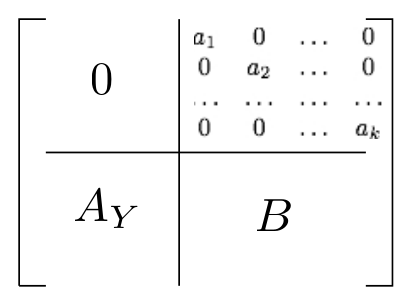
where $a_{i}$ , $1\leq a_{i}\leq s$ , corresponds to the coordinate of the first lattice point on the $i$ th edge of the simplex $Q$ . The matrix $A_{Y}$ is the matrix given by the first lattice points through the (corresponding) vertex of $P_{0}$ . A standard computation in linear algebra gives $\det(A)=\det(A_{Y})a_{1}\cdots a_{k}$ . It follows that $\det(A_{Y})=1$ and $a_{1}=\cdots=a_{k}=1$ .

Because each vertex of $P_{i}$ is the intersection of a smooth fiber with $P_{i}$ , we conclude that $P_{i}$ is smooth for all $i=0,\ldots,k$ . The equalities $a_{1}=\cdots=a_{k}=1$ show that all invariant fibers have edge length $s$ . Every special fiber (as a cycle) is a combination of invariant fibers. If there were a non reduced fiber $tF$ , then it should contain an invariant curve such that $tC$ is numerically equivalent to $C^{\prime}$ , where $C^{\prime}$ is an invariant curve in $s\Delta$ . Then, because $L\cdot C\geq s$ and $L\cdot C^{\prime}=s$ , we would have $t=1$ . Lemma 3.6 implies that the $P_{i}$ are smooth, and hence $Y$ is smooth. One can see this also from the standard fact that for every morphism with connected fibers between two normal toric varieties, the general fiber is necessarily toric [8, Lemma 1.2]. ∎

Observe that the hypothesis that $P^{s}$ is smooth in Lemma 3.6 above, is essential in order to prove that all fibers are reduced and embedded as Veronese varieties.

Toric projective bundles are isomorphic to projectivized bundles of a vector bundle, which necessarily splits as a sum of line bundles [8, Lemma 1.1]. We will denote the projectivized bundle by ${\mathbb{P}}_{Y}(L_{0}\oplus\cdots\oplus L_{k})$ , where $Y$ is the toric variety associated to $\Sigma$ .

Proposition 3.7.

Let $P_{0},\ldots,P_{k}\subset{\mathbb{R}}^{m}$ be strictly combinatorially equivalent polytopes such that

P^{s}:=\Cayley_{\Sigma}^{s}(P_{0},\ldots,P_{k})

is smooth. Then there are line bundles $L_{0},\cdots,L_{k}$ on $Y=X(\Sigma)$ such that the toric variety $X(\Sigma_{P^{s}})$ , defined by the inner normal fan $\Sigma_{P^{s}}$ of $P^{s}$ , is isomorphic to ${\mathbb{P}}_{Y}(L_{0}\oplus\cdots\oplus L_{k}).$

Proof.

Denote by $L$ the ample line bundle on $X(\Sigma_{P^{s}})$ associated to the given polytope $P^{s}$ . By Lemma 3.6, all fibers are isomorphic to ${\mathbb{P}}^{k}$ and thus $X(\Sigma_{P^{s}})$ has the structure of a projective bundle over $Y$ . Equivalently, $f_{*}(L)=L_{0}\oplus\cdots\oplus L_{k}$ and $X(\Sigma_{P^{s}})\cong{\mathbb{P}}_{Y}(L_{0}\oplus\cdots\oplus L_{k})$ , where $f\colon X(\Sigma_{P^{s}})\to Y$ . ∎

A complete description of the geometry of such varieties when $s=1$ is contained in [7, Section 3] and [13, 1.1].

Throughout the rest of the section we will always assume that $P^{s}=\Cayley^{s}_{\Sigma}(P_{0},\ldots,P_{k})$ is a smooth polytope. Denote as before by $(X,L)$ the associated polarized toric variety. Let $f\colon X\to Y$ be as above. The invariant curves on $X$ are of two types:

(1)

pullbacks $f^{*}V(\alpha_{i})$ of invariant curves from $Y$ , corresponding to the edges of $P_{i}$ ,
(2)

curves $V(\alpha_{F})$ contained in a fiber $F$ , corresponding to the edges on simplices $s\Delta^{k}$ .

Line bundles on $X$ can be written as $L=f^{*}(M)+a\xi$ , where $M$ is a line bundle on $Y$ and $\xi$ is the tautological line bundle on ${\mathbb{P}}_{Y}(L_{0}\oplus\ldots\oplus L_{k}).$

Because a line bundle on a nonsingular toric variety is spanned, respectively (very) ample, if and only if the intersection with all the invariant curves is non negative, respectively positive, there is a well understood spannedness and ampleness criterion, see [7, Prop. 2].

Lemma 3.8.

Let $L=f^{*}(M)+a\xi$ be a line bundle on ${\mathbb{P}}_{Y}(L_{0}\oplus\cdots\oplus L_{k})$ . Then for every curve of type $f^{*}V(\alpha_{i})$ , we have $L\cdot f^{*}V(\alpha_{i})=(M+sL_{i})\cdot V(\alpha_{i})$ , and for every curve $V(\alpha_{F})$ we have $V(\alpha_{F})\cdot L=a$ . Consequently

(1)

$L$ is ample if and only if $a\geq 1$ and $M+sL_{i}$ is ample for all $i$ ,
(2)

$L$ is spanned if and only if $a\geq 0$ and $M+sL_{i}$ are spanned for all $i$ .

Because the fibers of $\pi$ correspond to simplices $s\Delta_{k},$ and thus are embedded as $s$ -Veronese varieties, and because the line bundles $L_{i}$ are ample, we see that $P^{s}=\Cayley^{s}_{\Sigma}(P_{0},\ldots,P_{k})$ corresponds to the toric embedding

({\mathbb{P}}_{Y}(L_{0}\oplus\cdots\oplus L_{k}),s\xi).

Proposition 3.9.

Let $P^{s}=\Cayley^{s}_{\Sigma}(P_{0},\ldots,P_{k})$ be a smooth generalized strict Cayley polytope. Assume that $\dim P_{i}+1<\frac{k+1}{s}$ for all $i$ . Then $P^{s}$ is ${\mathbb{Q}}$ -normal, and

\textstyle\codeg_{\mathbb{Q}}(P^{s})=\tau(P^{s})=\frac{k+1}{s}.

Proof.

Recall that

X:=X(P^{s})={\mathbb{P}}_{Y}(L_{0}\oplus\cdots\oplus L_{k}),

where $L_{i}$ is ample on $Y:=X(\Sigma)$ , for $i=0,\ldots,k$ , and $P^{s}$ is the polytope defined by the line bundle $s\xi$ , where $\xi:=\xi_{L_{0}\oplus\cdots\oplus L_{k}}$ .

Recall also that the canonical line bundle on $X$ is $K_{X}=\pi^{*}(K_{Y}+L_{0}+\cdots+L_{k})-(k+1)\xi$ , where $\pi\colon X\to Y$ . It follows that

H:=bK_{X}+as\xi=\pi^{*}(b(K_{Y}+L_{0}+\cdots+L_{k}))+(as-b(k+1))\xi.

By Lemma 3.8, $H$ is spanned (resp. ample) if and only if $as-b(k+1)\geq 0$ (resp. $\geq 1$ ) and $b(K_{Y}+L_{0}+\cdots+L_{k})+sL_{i}$ is spanned (resp. ample).

Observe that, because $L_{i}$ is ample for each $i$ , $K_{Y}+L_{0}+\cdots+L_{k}$ is ample if $k+1>\dim P_{i}+1$ [12, Cor. 4.2 (ii)], which holds by assumption. It follows that, with the given hypotheses, we have

(i)

$H$ is spanned if and only if $\frac{a}{b}\geq\frac{k+1}{s}$
(ii)

$H$ is ample if and only if $\frac{a}{b}>\frac{k+1}{s}$ ,

and thus $\tau(P)=\frac{k+1}{s}$ .

Consider the projection map $\pi\colon{\mathbb{R}}^{n}\to{\mathbb{R}}^{k}$ such that $\pi(P)=s\Delta_{k}$ . Clearly, if $a,b$ are such that $(aP)^{(b)}\neq\emptyset$ , then for all points $m\in(aP)^{(b)}$ , $\pi(m)\in(as\Delta_{k})^{(b)}$ . This implies that $\frac{a}{b}\geq\codeg_{\mathbb{Q}}(s\Delta_{k})=\frac{k+1}{s}$ , and hence $\codeg_{\mathbb{Q}}(P)\geq\frac{k+1}{s}$ . Together with the inequality $\codeg_{\mathbb{Q}}(P)\leq\tau(P)=\frac{k+1}{s}$ , this proves

\textstyle\codeg_{\mathbb{Q}}(P)=\tau(P)=\frac{k+1}{s}.

∎

Remark 3.10.

Christian Haase showed us the following beautiful geometric argument to prove Proposition 3.9. As before, denote by $\Sigma$ the common normal fan of $P_{0},\dots,P_{k}$ and by $\Sigma(P^{s})$ the normal fan of $P^{s}$ . Consider the smooth toric varieties $X=X(\Sigma(P^{s}))$ and $Y=X(\Sigma)$ , and let $L$ denote the ample line bundle on $X$ with associated polytope $P^{s}$ and $L_{0},\dots,L_{k}$ the ample line bundles on $Y$ with associated polytopes $P_{0},\dots,P_{k}$ .

As $\tau(s\Delta_{k})=\frac{k+1}{s}>\tau(P_{i})$ , we have that an integer multiple of $L_{i}+\frac{s}{k+1}K_{Y}$ is ample on $Y$ for all $i=0,\ldots,k$ . Let $\rho_{1},\ldots,\rho_{\ell}$ be the primitive generators of the one dimensional cones in $\Sigma$ , so that

P_{i}\,=\,\cap_{j=1}^{\ell}H^{+}_{\rho_{j},-a_{ij}}.

Then the polytope

\cap_{j=1}^{\ell}H^{+}_{\rho_{j},-a_{ij}+\frac{s}{k+1}},

corresponding to the line bundle (with coefficients in ${\mathbb{Q}}$ ) $L_{i}+\frac{s}{k+1}K_{Y}$ , is combinatorially equivalent to $P_{i}$ , for all $i=0,\ldots,k$ . On the other hand, the polytope

\textstyle\{x=(x_{1},\ldots,x_{k})\in s\Delta_{k}\,|\,\sum_{i=1}^{k}x_{i}\leq s-\frac{s}{k+1},\,x_{i}\geq\frac{s}{k+1},\,\forall\,i=1,\ldots,k\}

equals the barycenter $v$ of the simplex $s\Delta_{k}$ . Hence the polytope associated to $L+\frac{s}{k+1}K_{X}$ reduces to the fiber over $v$ in $P^{s}$ , which can be identified with $\frac{1}{k+1}(P_{0}+\cdots+P_{k})$ , and no multiple of the corresponding line bundle is ample.

For any rational number $\frac{a}{b}>\frac{k+1}{s}$ , we have again that the polytope

\cap_{j=1}^{\ell}H^{+}_{\rho_{j},-a_{ij}+\frac{b}{a}}

is combinatorially equivalent to $P_{i}$ for all $i=0,\ldots,k$ . But now the polytope given by the points in $s\Delta_{k}$ at lattice distance $\frac{b}{a}$ from each of its facets is also combinatorially equivalent to $s\Delta_{k}$ , and therefore the polytope corresponding to $L+\frac{b}{a}K_{X}$ is combinatorially equivalent to $P^{s}$ . We conclude that $\tau(P^{s})=\frac{k+1}{s}$ , as wanted.

4. Classifying smooth lattice polytopes with high codegree

We now use the results in the previous sections to give the proof of Theorem 1.12.

Proof of Theorem 1.12. Let $(X,L)$ be the nonsingular toric variety and ample line bundle associated to $P$ .

Assume (1) holds. Because $P$ is ${\mathbb{Q}}$ -normal, Lemma 2.7 implies that the nef value map $\varphi:=\varphi_{P}$ is not birational. Set $\tau:=\tau(P)$ . Lemma 2.4 gives that $\tau>\codeg(P)-1\geq\frac{n+1}{2}$ . If $n$ is even and $P=\Delta_{\frac{n}{2}}\times\Delta_{\frac{n}{2}}$ , then $\codeg(P)=\frac{n}{2}+1<\frac{n+3}{2}$ . Therefore, Lemma 2.6 implies that $\tau$ is an integer and $\tau\geq\codeg(P)\geq\frac{n+3}{2}$ , and that $\varphi\colon X\to Y$ is a (non birational) contraction of an extremal ray in the nef cone $NE(X)$ of $X$ .

By [14, Cor. 2.5, p. 404], we know that $\varphi$ is flat, $Y$ is a smooth toric variety, and, since $X$ is smooth, a general fiber $F$ is isomorphic to ${\mathbb{P}}^{k}$ , where $k=\dim X-\dim Y$ . Under this isomorphism, $L|_{F}={\mathcal{O}}_{{\mathbb{P}}^{k}}(s)$ , for some positive integer $s$ . Let $\ell\subseteq F\cong{\mathbb{P}}^{k}$ be a line. Then, since $F$ , and hence $\ell$ , is contracted by $\varphi$ , we have

0=(K_{X}+\tau L)\cdot\ell=K_{X}\cdot\ell+\tau L\cdot\ell=K_{F}\cdot\ell+\tau s=-(k+1)+\tau s.

We therefore get

\textstyle\frac{n+1}{2}<\tau=\frac{k+1}{s}\leq\frac{n+1}{s},

which gives $s=1$ and $\tau=\codeg_{\mathbb{Q}}(P)=k+1\in{\mathbb{Z}}$ . By Lemma 2.4, we have $\tau\geq\codeg(P)$ . As $\codeg(P)\geq\codeg_{\mathbb{Q}}(P)$ , we get $\codeg(P)=k+1$ . Hence $k+1\geq\frac{n+3}{2}$ , so that $k>\frac{n}{2}$ .

Since $L^{k}\cdot F=1$ for a general fiber of $\varphi$ and $\varphi$ is flat, $L^{k}\cdot Z=1$ for every fiber $Z$ . Therefore all fibers are irreducible, reduced, and of degree one in the corresponding embedding. It follows that for every fiber $Z,$ $(Z,L|_{Z})\cong({\mathbb{P}}^{k},{\mathcal{O}}_{{\mathbb{P}}^{k}}(1)).$ Therefore $\varphi$ is a fiber bundle: $X={\mathbb{P}}_{Y}(\varphi_{*}L)$ , where $\varphi_{*}L$ is a rank $k+1$ vector bundle. Since $Y$ is toric, this bundle splits as a sum of line bundles $\varphi_{*}L=L_{0}\oplus\ldots\oplus L_{k}$ , and therefore $P$ is a strict Cayley polytope. Hence (1) implies (2).

Assume (2) holds. By Proposition 3.9 (with $s=1$ ), $P$ is ${\mathbb{Q}}$ -normal, and $\codeg_{\mathbb{Q}}(P)=\tau=k+1$ . Since $\codeg_{\mathbb{Q}}(P)$ is an integer, $\codeg(P)=\codeg_{\mathbb{Q}}(P)$ , hence $\codeg(P)=k+1>\frac{n}{2}+1$ , so $\codeg(P)\geq\frac{n+3}{2}$ . Therefore (1) holds.

The equivalence of (2) and (3) is essentially contained in [7]; here is a brief sketch of the proof.

Assume (2) holds. Since $k>\frac{n}{2}$ , $(X,L)$ is defective with defect $\delta\ =2k-n$ [11, Prop. 5.12, p. 369] hence $\delta=2\codeg(P)-2-n$ , since $\codeg(P)=k+1$ .

Assume (3) holds, so that $P$ is defective with defect $\delta=2\codeg(P)-2-n\geq 1$ . By [7, Thm. 2], then $P=\Cayley_{\Sigma}(P_{0},\ldots,P_{k})$ is a smooth strict Cayley polytope, with $k=\frac{n+\delta}{2}>\frac{n}{2}$ and $\codeg(P)=\frac{n+\delta}{2}+1=k+1$ . $\square$

We isolate the following result from the statement and proof of the previous theorem.

Corollary 4.1.

Let $P$ be a smooth ${\mathbb{Q}}$ -normal lattice polytope of dimension $n$ , and assume $\codeg(P)\geq\frac{n+3}{2}$ . Then, $\tau:=\tau(P)=\codeg(P)$ is an integer and the associated polarized toric variety $(X,L)$ is defective with defect $\delta=2\tau-2-n$ .

The classification of smooth ${\mathbb{Q}}$ -normal lattice polytopes of degree $0$ and $1$ follows from Theorem 1.12 (cf. [1] for the general case).

Corollary 4.2.

Assume $P$ is a smooth, ${\mathbb{Q}}$ -normal $n$ -dimensional lattice polytope. Then

(1)

$\deg(P)=0$ if and only if $P=\Delta_{n}$ ,
(2)

$\deg(P)=1$ if and only if $P={\rm Cayley}(P_{0},\ldots,P_{n-1})$ is a Lawrence prism (the $P_{i}$ are segments) or $P=2\Delta_{2}$ .

Proof.

(1) Because $\tau(P)>{\rm codeg}(P)-1=n\geq\frac{n+1}{2},$ Lemma 2.6Ê implies that $\varphi_{P}$ contracts a line. It follows that $\tau(P)$ is an integer, $\tau(P)\geq n+1$ and thus $\tau(P)={\rm codeg}(P)=n+1$ . Theorem 1.12 implies that $P$ is a strict Cayley polytope with $k=n$ . This is equivalent to $P=\Delta_{n}$ .

(2) For $n\geq 3$ the same argument as in (1) applies and gives that $P$ is Cayley with $k=n-1$ . Assume $n=2.$ Since $\codeg(P)=2$ , $P\neq\Delta_{2}$ and $P$ has no interior lattice points. Let $m$ be a vertex of $P$ . Because $P$ is smooth, the first lattice points on the two edges containing $m(\sigma)$ form a lattice basis. In this basis $m(\sigma)=(0,0)$ , and the lattice point $(1,1)$ is not an interior point of $P$ . Therefore there are only three possibilities: (i) One of the edges has length $>1$ , the other edge has length $1$ , and the point $(1,1)$ is on a third edge parallel to $\rho_{1}$ , which gives a strict Cayley polytope. (ii) Both edges have length $1$ , and $(1,1)$ is the fourth vertex, hence $P=\Delta_{1}\times\Delta_{1}=\Cayley_{\Sigma(\Delta_{1})}(\Delta_{1},\Delta_{1})$ . (iii) Both edges have length $2$ , and there is only one other edge containing $(1,1)$ . In this case $P=2\Delta_{2}.$ ∎

We close the paper with some loose ends. In the Introduction we conjectured that any smooth lattice polytope $P$ with $\codeg(P)\geq\frac{n+3}{2}$ is in fact ${\mathbb{Q}}$ -normal. This conjecture is supported by [3, 7.1.8], which suggests that for $n\leq 7$ , if $P$ is a smooth lattice polytope and $\codeg_{\mathbb{Q}}(P)>\frac{n}{2}$ , then $P$ is ${\mathbb{Q}}$ -normal. We also expect that without any smoothness assumptions, all lattice polytopes $P$ with $\codeg(P)\geq\frac{n+3}{2}$ are indeed Cayley polytopes.

Acknowledgements.

We thank the Institute for Mathematics and its Applications (IMA), Minneapolis, where this project began. We also thank the Department of Mathematics of KTH and the Göran Gustafsson Foundation, as well as the Center of Mathematics for Applications (CMA) and Department of Mathematics of the University of Oslo, for sponsoring several visits, during which this paper was completed. We are grateful to Eva Maria Feichtner and Bernd Sturmfels for calling our attention to the paper [1], and to Eduardo Cattani for useful discussions. We would also like to thank Christian Haase and Benjamin Nill for very interesting discussions, and for showing us the alternative proof in Remark 3.10. Finally, we would like to thank the referee for thoughtful and most helpful comments.

References

[1] Victor V. Batyrev and Benjamin Nill. Multiples of lattice polytopes without interior lattice points. Moscow Math. J., 7(2):195–207, 2007.
[2] Mauro C. Beltrametti and Andrew J. Sommese. On the adjunction theoretic classification of polarized varieties. J. reine angew. Math. 427:157–192, 1992.
[3] Mauro C. Beltrametti and Andrew J. Sommese. The adjunction theory of complex projective varieties, de Gruyter Expositions in Mathematics, Vol. 16. Walter de Gruyter & Co., Berlin, 1995.
[4] Mauro C. Beltrametti, Andrew J. Sommese, and Jarosław A. Wiśniewski. Results on varieties with many lines and their applications to adjunction theory. In Complex algebraic varieties (Bayreuth, 1990), pp. 16–38. Lecture Notes in Math., 1507, Springer, Berlin, 1992.
[5] Cinzia Casagrande and Sandra Di Rocco. Projective Q-factorial toric varieties covered by lines. Comm. Contemp. Math., 10(3):363–389, 2008.
[6] Herbert Clemens, János Kollàr, and Shigefumi Mori. Higher-dimensional complex geometry. Astérisque No. 166, 1988.
[7] Sandra Di Rocco. Projective duality of toric manifolds and defect polytopes. Proc. London Math. Soc. (3), 93(1):85–104, 2006.
[8] Sandra Di Rocco and Andrew J. Sommese. Chern numbers of ample vector bundles on toric surfaces. Trans. Amer. Math. Soc., 356(2):587–598, 2004.
[9] Yujiro Kawamata. The cone of curves of algebraic varieties. Ann. of Math. (2), 119(3):603–633, 1984.
[10] Christian Haase, Benjamin Nill, and Sam Payne. Cayley decompositions of lattice polytopes and upper bounds for $h^{*}$ -polynomials. Preprint, arXiv:0804.3667, 2008. (To appear in J. reine angew. Math.)
[11] Antonio Lanteri and Daniele Struppa. Projective manifolds whose topology is strongly reflected in their hyperplane sections. Geom. Dedicata, 21(3):357–374, 1986.
[12] Mircea Mustaţă. Vanishing theorems on toric varieties. Tohoku Math. J. (2), 54(3):451–470, 2002.
[13] Tadao Oda. Convex bodies and algebraic geometry. Ergebnisse der Mathematik und ihrer Grenzgebiete (3), Vol. 15, Springer-Verlag, Berlin 1988.
[14] Miles Reid. Decomposition of toric morphisms. In Arithmetic and geometry, Vol. II, pp. 395–418, Progr. Math., 36, Birkhäuser Boston, Boston, MA, 1983.
[15] Günter M. Ziegler. Lectures on polytopes. Graduate Texts in Mathematics, 152. Springer-Verlag, New York, 1995.