Dynamics and constraints of the Unified Dark Matter flat cosmologies

If we combine eq.(13) together with the initial parameterization [see eq.(8)] we immediately obtain the following expressions:

and after some algebra the evolution of the scalar field becomes:

Using eqs. (5) and (16) one can prove that

Now the range of $\Psi$-values for which the UDM scalar field is well defined [due to eq.(16)] is: $\Psi\in(-1,1)$. Evidently, when the system reaches at the critical point $\phi=0$ then $\Psi(t_{m})=0$ (or $V_{min}=4\omega^{2}_{1}\kappa/3$). For this to be the case we must have $t_{m}=-\theta_{1}/\omega_{1}$ and therefore, $\theta_{1}<0$.

Inserting eq.(13) into eq.(10) the scale factor, normalized to unity at the present epoch, evolves in time as

where $t_{0}$ is the present age of the universe in billion years. The constant $\theta_{1}$ is related to $\theta_{2}$ because at the singularity ($t=0$), the scale factor has to be exactly zero [see eq.(18)]. After some algebra, we find that

Furthermore, we investigate the circumstances under which an inflection point exists and therefore have an acceleration phase of the scale factor. This crucial period in the cosmic history corresponds to $\ddot{a}(t_{I})=0$ which implies that the condition

should contain roots which are real and such that $a\in(0,1)$. The above equation is solvable because for $c_{1},c_{2}>0$ the potential energy [$V(\phi)$] takes only positive values. Knowing the integration constants ($\omega_{1},\theta_{1},\omega_{2},\theta_{2}$), of the current dynamical problem we can calculate the inflection point by solving numerically the following equation:

with

where $\nu_{1}=1$ and $\nu_{2}=-\sqrt{\kappa}$.

In addition, the Hubble function predicted by the UDM model can be viewed as the sum of basic hyperbolic functions:

with

where $H_{0}$ is the Hubble constant. In this work we use $H_{0}=100h$Kms^-1Mpc^-1 with $h=0.72$ [45] or $H_{0}=h/9.778\simeq 0.0736$Gyr^-1 corresponding to $t_{0}\approx H^{-1}_{0}\simeq 13.6$Gyr. Also we can relate the frequency $\omega_{2}$ of the hyperbolic oscillator in the $x_{2}$ axis with the well known cosmological parameters. Indeed, $\omega_{2}$ is given by

while $\theta_{1}\propto H_{0}t_{0}$ has no units. Notice that, $\Omega_{m}$ is the matter density at the present time.

Without wanting to appear too pedagogical, we remind the reader of some basic elements of the concordance $\Lambda$-cosmology. In this framework, the normalized scale factor of the universe is

The Hubble function is written as

Comparing the $\Lambda$ model with the observational data (we sample $\Omega_{m}\in[0.1,1]$ in steps of 0.01) we find that the best fit value is $\Omega_{m}=0.26\pm 0.01$ with $\chi_{tot}^{2}(\Omega_{m})\simeq 195$ (${\rm dof}=192$) in a very good agreement with the 5 years WMAP data [4]. The inflection point takes place at

Therefore, we estimate $\omega_{2}\simeq 1.29H_{0}\simeq 0.095$Gyr^-1, $t^{\Lambda}_{I}\simeq 0.51t_{0}$ and $a^{\Lambda}_{I}\simeq 0.56$. The deceleration parameter at the present time is $q_{0}\equiv-\ddot{a}/\dot{a}^{2}|_{a=1}\simeq-0.61$.

In this case we use a simple parameterization for the dark energy equation of state parameter which is based on a Taylor expansion around the present time (see Chevallier & Polarski [46] and Linder [47], hereafter CPL)

The Hubble parameter is given by:

where ${\rm w}_{0}$ and ${\rm w}_{1}$ are constants. We sample the unknown parameters as follows: ${\rm w}_{0}\in[-2,-0.4]$ and ${\rm w}_{1}\in[-2.6,2.6]$ in steps of 0.01. We find that for $\Omega_{m}=0.26$ the overall likelihood function peaks at ${\rm w}_{0}=-1.20^{+0.28}_{-0.20}$ and ${\rm w}_{1}=1.14^{+1.0}_{-1.9}$ while the corresponding $\chi_{tot}^{2}({\rm w}_{0},{\rm w}_{1})$ is 193.6 (${\rm dof}=191$). The deceleration parameter at the present time is $q_{0}\simeq-0.83$.

Let us consider now a completely different model namely the variable Chaplygin gas (herafter VCG) which corresponds to a Born-Infeld tachyon action [48, 49]. Recently, an interesting family of Chaplygin gas models was found to be consistent with the current observational data [50]. In the framework of a spatially flat FLRW metric, it can be shown that the Hubble function takes the following formula:

where $\Omega_{b}\simeq 0.021h^{-2}$ is the density parameter for the baryonic matter [51] and $B_{s}\in[0.01,0.51]$ in steps of 0.01 and $n\in[-4,4]$ in steps of 0.02. The corresponding effective equation of state parameter ${\rm w}(a)=P_{DE}/\rho_{DE}$ is related to $H(a)$ according to

while the effective matter density parameter is: $\Omega^{eff}_{m}=\Omega_{b}+(1-\Omega_{b})\sqrt{B_{s}}$. We find that the best fit parameters are $B_{s}=0.07\pm 0.02$ and $n=1.06\pm 0.33$ ($\Omega^{eff}_{m}\simeq 0.29$) with $\chi_{tot}^{2}(B_{s},n)=193.7$ (${\rm dof}=191$) and the present value of the deceleration parameter is $q_{0}\simeq-0.60$.

In order to predict analytically the time evolution of the main cosmological functions [$\phi(t)$, $a(t)$, $H(t)$ and ${\rm w}(t)$] we have to define the corresponding unknown constants of the problem ($\omega_{1},\theta_{1},\omega_{2},\theta_{2}$). At the same time, from the restrictions found in section 3 (see eqs. 12, 19 and 24), we can reduce the parameter space to $(\Omega_{m},\theta_{1})$. We do so by fitting the predictions of the UDM cosmological model and recent observational data. Here, we use $\Omega_{m}\in[0.1,1]$ and $\theta_{1}\in[-1,0]$ in steps of 0.01.

Figure 1 (thin dashed lines) shows the 1$\sigma$, 2$\sigma$ and 3$\sigma$ confidence levels in the $(\Omega_{m},|\theta_{1}|)$ plane when using BAOs. Obviously, the $\theta_{1}$ parameter is not constrained by this analysis and all the values in the interval $-1\leq\theta_{1}\leq 0$ are acceptable. However, the BAOs statistical analysis puts constraints on the matter density parameter $\Omega_{m}\simeq 0.25$.

Therefore, in order to put further constraints on $\theta_{1}$ we additionally utilize the SNIa data. In figure 1 (thick solid lines), we present the SNIa likelihood contours and we find that the best fit solution is $\Omega_{m}\simeq 0.4$ and $\theta_{1}\simeq-0.05$. The joint likelihood function peaks at $\Omega_{m}=0.25^{+0.02}_{-0.01}$ and $\theta_{1}=-0.39^{+0.04}_{-0.08}$ ($\theta_{2}\simeq 0.54$) with $\chi_{tot}^{2}(\Omega_{m},|\theta_{1}|)\simeq 194.1$ (${\rm dof}=191$). Note that the errors of the fitted parameters represent $1\sigma$ uncertainties. In the insert plot of figure 1 we provide the solutions (circles-BAOs and triangles-SNIa) within $1\sigma$ contours in the $(\Omega_{m},\phi_{0})$ plane, where $\phi_{0}$ is the present value of the scalar field. The corresponding best fit value of the scalar field (see eqs. 15 and 16) is $\phi_{0}\simeq 0.42$ or $0.084$ in Planck units ($G=c\equiv 1$), while the frequencies are $\omega_{1}\simeq 0.067$Gyr^-1 and $\omega_{2}\simeq 0.095$Gyr^-1. It is interesting to mention that although the frequency ($\omega_{1}\sim 0.9H_{0}$) of the hyperbolic oscillator in the $x_{1}$ axis is somewhat less than the present expansion rate of the universe, the $\omega_{2}$ is equal to the value predicted by the $\Lambda$ cosmology (see section 4.1).

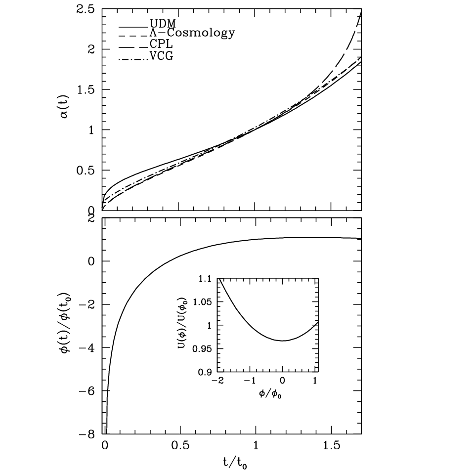
Knowing now the parameter space ($\omega_{1},\theta_{1},\omega_{2},\theta_{2}$) we investigate, in more detail, the correspondence of the UDM model with the different dark energy models (see sections 4.1, 4.2 and 4.3) in order to show the extent to which they compare. Our analysis provides an evolution of the UDM scale factor seen in the upper panel of figure 2 as the solid line, which closely resembles, especially at late times ($0.6<a\leq 1.5$), the corresponding scale factor of the $\Lambda$ (short dashed), VCG (dot dashed), and CPL (long dashed). Note that the UDM deceleration parameter at the present time is $q_{0}\simeq-0.62$. However, for $a>1.5$, the CPL and the VCG scale factors evolve more rapidly than the other two models (UDM and $\Lambda$ cosmology). Also it is clear that an inflection point [$\ddot{a}(t_{I})=0$] is present in the evolution of the UDM scale factor. The UDM inflection point is located at $t_{I}\simeq 0.46t_{0}$ which corresponds to $a_{I}\simeq 0.61$ and is somewhat different than the value predicted from the usual $\Lambda$ cosmology (see section 4.1). Before the inflection point, the UDM appears to be more decelerated from the other three dark energy cosmological models due to the fact that the second term [$\propto{\rm sinh}^{2}(\omega_{1}t+\theta_{1}$)] in eq.(18) plays an important role. From figure 2 it becomes clear that the UDM model reaches a maximum deviation from the other three dark energy models prior to $a\sim 0.15$ ($z\sim 5.5$). In order to investigate whether the expansion of the observed universe follows such a possibility we need a visible distance indicator (better observations) at redshifts $z>2$.

The evolution of the scalar field is presented in the bottom panel of figure 2, while in the insert figure we plot the scalar field dependence of the potential energy normalized to unity at the present time. As we have stated in section 3.1 there is one minimum at $\phi=0$ that corresponds to $t_{m}=-\theta_{1}/\omega_{1}\sim 0.4t_{0}$. To conclude, we plot in figure 3 the relative deviations of the distance modulus, $\Delta(m-M)$, of the dark energy models used here from the traditional $\Lambda$ cosmology. Notice that the open points represent the following deviation: $(m-M)_{SNIa}-(m-M)_{\Lambda}$. Within the SNIa redshift range $0.016\leq z\leq 1.775$ ($0.360\leq a\leq 0.984$) the VCG distance modulus is close to the $\Lambda$ one. The largest deviations of the distance moduli occur at redshifts around 0.5-1 for the UDM and 1.1-1.5 for the CPL model respectively.

We would like to end this section with a discussion on the dark energy equation of state. As we have stated already in the introduction, there is a possibility for the equation of state parameter to be a function of time rather than a constant ratio between the pressure and the energy density. Within the framework of the scalar field cosmology the equation of state parameter is derived from the field model and in general it is a complicated function of time, even when the potential is written as a simple function of the scalar field. In our case we have

or else (see eqs.16, 17)

Note that $\Lambda-$models can be described by scalar models with ${\rm w}$ strictly equal to -1. Using our best fit parameters we present in left panel of figure 4, the equation of state parameter as a function of the scale factor for the different dark energy models. The UDM model (solid line) is the only case that provides positive values for the equation of state parameter at early epochs. We have checked the UDM scenario against the cosmic coincidence problem (why the matter energy density and the dark energy density are of the same order at the present epoch) by utilizing the basic tests proposed by [41]. These are: (a) at early enough times the equation of state parameter tends to its maximum value, ${\rm w}\longrightarrow+1$, which means that the dark energy density initially takes large values. So as long as the scalar field rolls down the potential energy, $V(\phi)$, decreases rapidly and the kinetic energy $T_{\phi}={\dot{\phi}}^{2}/2$ takes a large value, (b) then $\phi$ continues to roll down, the dark energy density decreases and the equation of state parameter remains close to unity for a quite long period of time ($a<0.2$) and (c) for $0.2\leq a\leq 0.95$ the equation of state parameter is a decreasing function of time and it becomes negative at $a>0.56$. Before that epoch, the potential energy of the scalar field remains less than the kinetic energy (see the insert plot in the left panel of figure 4) and the equation of state parameter (or the scalar field) resembles background matter. In a special case where ${\rm w}=0$ [or $T_{\phi}\simeq V(\phi)$] the equation of state behaves exactly like that of pressure-less matter. For ${\rm w}=-1/3$ we reach the same expansion as in an open universe, because the dark energy density evolves as $a^{-2}$ and has no effect on $\ddot{a}$. In fact, we verify that prior to the inflection point ${\rm w}(t_{I})\simeq-0.334$, which means that after $t_{I}$ the accelerating expansion of the Universe starts. Finally, ${\rm w}\simeq-1$ close to the present epoch $a\sim 1$ and the scalar field is effectively frozen (the same situation seems to hold also in the limit $a\gg 1$). This is to be expected because at this period the scalar field varies slowly with time (see the insert panel of figure 4), so that $T_{\phi}\ll V(\phi)$ and the dark energy fluid asymptotically reaching the de-Sitter regime (cosmological constant).

In order to conclude this discussion, it is interesting to point out that we also investigate the sensitivity of the above results to the matter density parameter. As an example, in the right panel of figure 4 we present the evolution of the equation of state parameter for $(\Omega_{m},\theta_{1})=(0.73,-1)$ [upper line] and $(\Omega_{m},\theta_{1})=(0.19,-0.1)$ [bottom line]. We confirm that in the range $\Omega_{m}\in(0.19,0.73)$ and $\theta_{1}\in(-1,-0.1)$ the general behavior (described before) of the functional form of the equation of state parameter is an intermediate case between the above lines for $a\leq 1$ and thus it depends weakly on the values of the parameter space ($\Omega_{m},\theta_{1}$). Therefore, our main cosmological results for the UDM scenario persist for all physical values of $\Omega_{m}$ and it strongly indicates that the UDM model over-passes the cosmic coincidence problem.

The evolution equation of the growth factor for models where the dark energy fluid has a vanishing anisotropic stress and the matter fluid is not coupled to other matter species is given by ([52], [53], [54]):

where $N={\rm ln}a$ and $\Omega_{m}(a)=\Omega_{m}a^{-3}H^{2}_{0}/H^{2}(a)$. Useful expressions of the growth factor can be found for the $\Lambda$CDM cosmology in [52], for the quintessence scenario (${\rm w}=const$) in [55], [56], [57], [58], for dark energy models with a time varying equation of state in [59] and for the scalar tensor models in [60]. In the upper panel of figure 5 we present the growth factor evolution which is derived by solving numerically eq. (38), for the four dark energy models (including the UDM). Note that the growth factors are normalized to unity at the present time. The behavior of the UDM growth factor (solid line) has the expected form, i.e. it is an increasing function of the scale factor. Also we find that the growth factor in the UDM model is almost an intermediate case between the VCG (dot dashed line) and CPL (long dashed line) models respectively. In the bottom panel of figure 5 we show the deviation, $(1-D_{DE}/D_{\Lambda})\%$, of the growth factors $D_{DE}(a)$ for the current dark energy models with respect to the $\Lambda$ solution $D_{\Lambda}(a)$. Assuming now that clusters have formed prior to the epoch of $z_{\rm f}\simeq 1.4$ ($a_{\rm f}\sim 0.42$), in which the most distant cluster has been found [69], the UDM scenario (open triangles) deviates from the $\Lambda$ solution by $4.2\%$ while the CPL (open circles) and VCG (solid squares) deviates by $-1.5\%$ and $5.1\%$ respectively. Also at the $\Lambda$-inflection point ($a^{\Lambda}_{I}\simeq 0.56$) we find the following results: (i) UDM-$\Lambda$ $3.3\%$, (ii) CPL-$\Lambda$ $-0.4\%$ and (iii) VCG-$\Lambda$ $3.2\%$. To conclude this discussion it is obvious that for $a\geq 0.7$ the UDM growth factor tends to the $\Lambda$ solution (the same situation holds for the CPL model but with $a\geq 0.55$).

The so called spherical collapse model, which has a long history in cosmology, is a simple but still a fundamental tool for understanding how a small spherical patch [with radius $R(t)$] of homogeneous overdensity forms a bound system via gravitation instability [61]. From now on, we will call $a_{\rm t}$ the scale factor of the universe where the overdensity reaches its maximum expansion ($\dot{R}=0$) and $a_{\rm f}$ the scale factor in which the sphere virializes, while $R_{\rm t}$ and $R_{\rm f}$ the corresponding radii of the spherical overdensity. Note that in the spherical region, $\rho_{mc}\propto R^{-3}$ is the matter density while $\rho_{\phi_{c}}$ will denote the corresponding density of the dark energy. In order to address the issue of the dark energy in the gravitationally bound systems (clusters of galaxies) we can consider the following assumptions: (i) clustered dark energy considering that that the whole system virializes (matter and dark energy), (ii) the dark energy remains clustered but now only the matter virializes and (iii) the dark energy remains homogeneous and only the matter virializes (for more details see [62], [63] [64] and [65]). Note, that in this work we are using the third possibility.

Here we review only some basic concepts of the problem based on the assumption that the dark energy component under a scale of galaxy clusters can be treated as being homogeneous: $\rho_{\phi_{c}}(t)=\rho_{\phi}(t)$, $\phi_{c}(t)=\phi(t)$ and ${\rm w}_{c}(t)={\rm w}(t)$. In general the evolution of the spherical perturbations as the latter decouple from the background expansion is given by the Raychaudhuri equation:

Now within the cluster region the evolution of the dark energy component is written as (see [62])

while if we consider a scalar field the above equation becomes

where

Figure 6 presents examples of $R(t)$ obtained for the UDM (solid line) and for the concordance $\Lambda$ model (dashed line). The time needed for a spherical shell to re-collapse is twice the turn-around time, $t_{\rm f}\simeq 2t_{\rm t}$.

On the other hand, utilizing both the virial theorem and the energy conservation we reach to the following condition:

where $U_{G}=-3GM^{2}/5R$ is the potential energy and $U_{\phi_{c}}=-4\pi GM(1+3{\rm w}_{c})\rho_{\phi_{c}}R^{2}/5$ is the potential energy associated with the dark energy for the spherical overdensity (see [62] and [63]; in our case $4\pi G\equiv 1/2$). Using the above formulation we can obtain a cubic equation that relates the ratio between the virial $R_{\rm f}$ and the turn-around outer radius $R_{\rm t}$ the so called collapse factor ($\lambda=R_{\rm f}/R_{\rm t}$). Notice that eq.(43) is valid when the ratio of the system’s dark energy to the matter’s densities at the time of the turn-around takes relatively small values [64]. Of course in the case of ${\rm w}_{c}=-1$ the above expressions get the usual form for $\Lambda$ cosmology ([57], [66]) while for an Einstein-de Sitter model ($\Omega_{m}=1$) we have $\lambda=1/2$.

Finally solving numerically eq.(43) [it can be done also analytically] we calculate the collapse factor. In particular, figure 7 shows the behavior of the collapse factor for the current cosmological models starting from the UDM (solid line), $\Lambda$ (short dashed), VCG (dot dashed), and CPL (long dashed). We find that the collapse factor lies in the range $0.43\leq\lambda\leq 0.50$ in agreement with previous studies ( [57], [62], [63], [64], [67], [68], [65]). Prior to the cluster formation epoch ($z_{\rm f}\simeq 1.4$) the UDM scenario, appears to produce more bound systems with respect to the other dark energy models. Indeed, we find the following values: $\lambda_{UDM}\simeq 0.44$, $\lambda_{\Lambda}\simeq 0.49$, $\lambda_{CPL}\simeq 0.48$ and $\lambda_{VCG}\simeq 0.50$. Also it becomes clear that the UDM collapse factor decreases slowly with the redshift of virialization $z_{f}$, due to its positive equation of state parameter. This is also incorporated by the fact that at early epochs the cosmic expansion of the UDM model is much more decelerated than in the other three dark energy models. The latter result is in agreement with those obtained by [62]. They found a similar behavior for the collapse factor by considering several potentials with an exponential phase.