Time dependent simulation of the Driven Lid Cavity at High Reynolds Number
Abstract
In this work, numerical solutions of the two dimensional time dependent incompressible flow, in a driven cavity at high Reynolds number , are presented. At high , there is a controversy. Some studies predicted that the flow is steady, others found time dependent non-steady flow, either periodic or aperiodic. In this study, the driven lid cavity is successfully solved using a very fine grid mesh, for up to . We discretize the Vorticity-Stream formulation of the Navier-Stokes equation with the SSPRK(5,4) scheme in a grid. Using this very fine grid, the results obtained converge to a stationary solution. Detailed results for between and are presented. The driven lid cavity problem is solved with a NVIDIA GPU using the CUDA programming environment with double precision.
Keywords:
Driven Lid Cavity Flow , 2-D Time Dependent Incompressible N-S Equation , Fine Grid , Reynolds Number , CUDA1 Introduction
The driven lid cavity flow is one of the most studied problems of the physics of fluids. The simple geometry makes the problem easy to solve numerically and apply boundary conditions. Despite being a problem rather studied, there are still some questions and controversy about what happens at high Reynolds numbers.
In the literature it is possible to find numerous studies about the driven cavity flow, however the nature of the flow at high Reynolds number is still not agreed upon. Driven cavity flow serve as a benchmark problem for numerical methods in terms of numerical efficiency and accuracy. Erturk [1] grouped these numerical studies into three categories. In the first category are the studies with numerical solutions of 2-D steady incompressible flow at high Reynolds numbers. Some of these studies are Erturk et. al. [2], Erturk and Gokcol [3], Barragy and Carey [4], Schreiber and Keller [5], Benjamin and Denny [6], Liao and Zhu [7], Ghia et. al. [8] for . Barragy and Carey [4] have also presented solutions for . Erturk et. al. [2] and also Erturk and Gokcol [3] have presented steady solutions up to . In the second category we have the studies about hydrodynamic stability analysis, Fortin et. al. [9], Gervais et. al. [10], Sahin and Owens [11] and Abouhamza and Pierre [12]. And the third category includes the studies about the steady to unsteady transition flow through a Direct Numerical Simulation (DNS) and the transition Reynolds number. Some of the studies found in the literature are Auteri, Parolini and Quartepelle [13], Peng, Shiau and Hwang [14], Tiesinga, Wubs and Veldman [15], Poliashenko and Aidun [16], Cazemier, Verstappen and Veldman [17], Goyon [18], Wan, Zhou and Wei [19] and Liffman [20].
Erturk [21] studied the numerical solutions of 2-D steady flow, with time independent equations, for and found that at high Reynolds numbers the solutions obtained depend of the mesh spacing. For coarse meshes, at high Reynolds numbers, he found no convergence. But for a fine grid he finds a steady solution. Thus he claimed that the true solution is steady and to be found numerically a very fine grid is needed.
Zhen-Hua et al. [22] with multi-relaxation-time (MRT model) lattice Boltzmann method obtained solutions for up to , but the grid used () in the MRT model are coarse compared to the article of Erturk, and the solutions obtained by them are not steady.
Notice that the existence of solutions to the stationary flow equation, does not necessarily imply that the natural solution is stationary. Let us illustrate this claim with the well known case of metastable water. At the normal pressure and at temperatures below freezing, two phases of water, i.e., two solutions of the non-linear equations for the water, exist. The stable solution is composed of solid water (ice) and the metastable is composed of supercooled water. In the same way the existence of a stationary solution to the flow equations, does not necessarily exclude the existence of a second, unsteady, solution. The solution of the time-dependent equation is necessary to discriminate which is the true solution, occurring naturally in the lab.
Since different authors find different solutions, in this paper we examine if for high Reynolds numbers as high as the numerical solutions of 2-D time dependent incompressible flow in a driven cavity become steady after a given time. Importantly, our equations are time-dependent, and our grid is very fine, thus we expect to obtain the true solution. We use the vorticity-stream function formulation to the Navier-Stokes equation.
This study is divided in five sections. The first section, the objective is presented and the existing works on the subject. In the second section, we present the theory and the fundamental equations used in the numeric calculations. In the third section, we describe the driven lid cavity problem, numeric equations, boundary conditions and the algorithm used. In the section four, we present the results and a comparison with existing studies about the cavity flow. Finally, in the section five, we present the conclusions about this study.
2 Vorticity-Stream Function Formulation
The fundamental equations of fluid dynamics are based on three universal laws of conservation: mass, moment and energy conservation. In general, there are two ways to solve numerically the Navier-Stokes equations. The first is proceeding with primitive variables formulation, , e . The second is using the vorticity-stream function approach.
Using the stream function, and the vorticity, , in place of the primitive variables , e , where these quantities are defined by:
| (1) |
and
| (2) |
The main reason for enter the stream function is that, for runoffs in which and are constants, the equation of continuity is satisfied.
The vorticity-stream function is given by
| (4) | ||||
| (5) |
where is the fluid velocity, the pressure, the fluid density and kinematic viscosity. The kinematic viscosity is given by:
| (6) |
where is the viscosity.
3 Numerical Method
In this section we present the driven lid cavity problem, the numerical equations, the boundary conditions and the algorithm. In the figure 1 is represented the outline problem to study. The top of the wall cavity moves with speed .

Numeric vorticity equation is given by:
| (7) |
with
| (8) | |||||
The five stage fourth order SSPRK developed by Ruuth and Spiteri, [23] , and guaranteed optimal [24], is given by:
| (9) | ||||
| (10) | ||||
| (11) | ||||
| (12) | ||||
| (13) | ||||
To get the stream function, we apply the fourth order method, [3], to solve the Poisson equation (3),
| (14) |
To solve the fourth order Stream equation, we use the Successive Over Relaxation method (SOR), since this method converge much faster than the traditional methods (methods of Jacobi and Gauss-Seidel). The idea is to use the available current estimates from other locations () when they become available and use the estimates of current positions () to improve the estimative of :
| (15) |
where is the relaxation parameter, and
| (16) | |||||
| (17) | |||||
| (18) | |||||
| (19) | |||||
| (20) | |||||
| (21) |
To obtain the velocity ( e ) it is only need to numerically solve the equation (2),
| (22) |
3.1 Boundary Conditions
The boundary conditions in the four walls are given by:
- •
left and right walls:
(23) - •
top and bottom walls:
(24)
where is the uniform velocity for the translation of the top wall and zero for the other three walls.
In order to solve equation (13), Thom’s method is used for calculating vorticity on the boundaries, therefore the boundary conditions are given by
| (25) |
3.2 Algorithm
An algorithm for solving the problem of the driven lid cavity using the vorticity-stream function approach is given by the scheme in figure 2.
To ensure the stability and convergence of the algorithm, should be small enough to a given viscosity, , and resolution of the grid, . The Reynolds number, , can be calculated using the kinematic viscosity, , and the conditions of the cavity:
in the following calculations it was considered:
Using this values, it’s the same using dimensionless variables.
In this study, we defined by the following equations
| (26) | |||||
| (27) |
for stream function and vorticity respectively, as convergence criteria to the steady state.
4 Results
In this work, we present results of the cavity flow from up to .
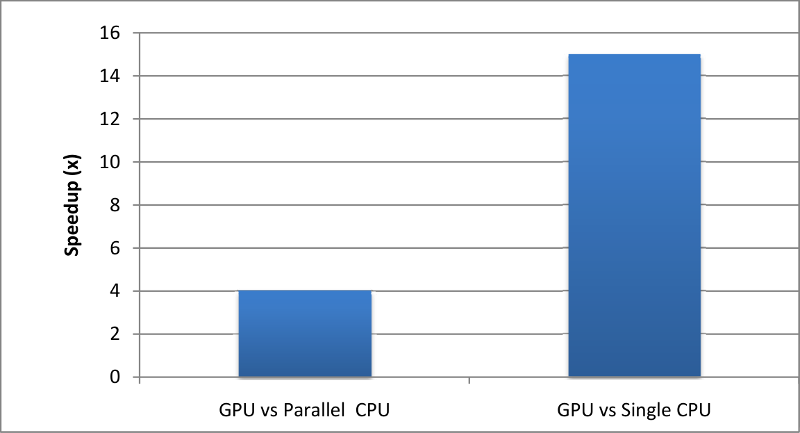
The numerical code was written for use in CPU’s (Intel(R) Core(TM)2 Quad CPU Q9450 @ 2.66GHz) and in GPU’s (NVIDIA GEFORCE 280 GTX GPU with double precision capabilities). For the CPU, we use OPENMP with C language and for GPU we use CUDA language. Most of the GPU’s only support single precision but the recent GPU’s have included support for double precision, although using double precision is almost eight times slower than single precision. Nevertheless, the GPU used is faster than the most recent Intel Quad core. Figure 3 summarizes our GPU code performance relative to the serial CPU version of our code and CPU parallel code performance relative to the serial CPU version of our code using double precision in all cases. In the parallel CPU version code we tested it in a Quad Core CPU with OPENMP.
In order to obtain a good convergence of the method we need to choose an appropriate value for the parameter, the relaxation parameter, in equation (15). We make several tests in order to see which value is the best and this parameter varies from 0.8 to 0.1 as the Reynolds number increase.
Using the algorithm described above, we started with a grid of points for and and the solution converges to a steady state in time.
For we obtain a solution that converges to a steady state with a grid of . With this small lattice we cannot obtain a solution for the Reynolds number above . Erturk et. al. [2] said that they have to use a grid of for . So, when we use a grid of for , we obtain a steady solution up to . The choice of this grid is due to the GPU architecture. Table 1 shows the grid mesh used at various Reynolds numbers for the final results. For up to , the algorithm ended when the value obtained by and were less than and for stream function and vorticity respectively. For and , the values considered for and were and . Such values are more than satisfactory, demonstrating that the solution converges to a steady state.
The figure 4 shows the boundary conditions and a schematic of the vortices generated in the driven cavity flow. In this figure, the abbreviations TL, BL and BR refer to top left, bottom left and bottom right corners of the cavity, respectively, and the number following these abbreviations to the vortices that appear in the flow, numbered according to size, Erturk [21].

Figures 5 to 9a show the stream function contours and Figure 11 the vorticity contours of the cavity flow up to . In the figure 5 are represented the stream function contours for , according to figure 4, all the vortices appear except the BL3 and TL2. This result is in agreement with the result obtained by Erturk [1]. For , figure 6, all the vortices appear except the TL2. For , all the vortices can be seen. These contour figures show that, the fine grid mesh provides very smooth solutions at high Reynolds numbers.


5 Conclusion
Numerical solutions of 2-D time dependent incompressible flow at high Reynolds numbers in a driven cavity are presented. The numerical equations are solved computationally using the numerical method above. For the Reynolds numbers studied, up to , the solution converges to a stationary state when using a very fine grid.
Based on the papers of Erturk et. al. [2], Erturk [1] and in this study, we conclude that in order to obtain a steady solution for the driven cavity flow, a very fine grid mesh is necessary when high Reynolds numbers are considered and also at high Reynolds numbers when a coarse grid mesh is used then the solution oscillates. This happens because a coarse mesh is not able to include the very small vortices at the corners.
According to Erturk [1], the studies that presented unsteady solutions of driven cavity flow using Direct Numerical Simulations (DNS) ([13, 17, 18, 20, 14, 16, 15, 19]) have experienced the same type of numerical oscillations because they have used a coarse mesh. With this study we agreed with Erturk [1]. In all of the Direct Numerical Simulation studies on the driven cavity flow found in the literature ([13, 17, 18, 20, 14, 16, 15, 19]), the maximum number of grid points used is less than . Therefore, the periodic solutions found in [13, 17, 18, 20, 14, 16, 15, 19] are similar to the false periodic solutions observed by Erturk et. al. [2] and Erturk [1] when a coarse grid mesh is used.
Acknowledgments
This study was possible due to the computer cluster funded by FCT grants PDCT/FP/63923/2005 and POCI/FP/81933/2007.
References
- [1] E. Erturk, Discussions on driven cavity flow, Accepted for publication in: Int. Journal for Numerical Methods in Fluids (2008) http://web.gyte.edu.tr/enerji/ercanerturk/drivencavity/sor/manuscript.h%tm.
- [2] E. Erturk, T. C. Corke, C. Gokcol, Numerical solutions of 2-D steady incompressible driven cavity flow at high Reynolds numbers, International Journal for Numerical Methods in Fluids 48 (2005) 747–774.
- [3] E. Erturk, C. Gokcol, Fourth order compact formulation of Navier-Stokes equations and driven cavity flow at high Reynolds numbers, International Journal for Numerical Methods in Fluids 50 (2006) 421–436.
- [4] E. Barragy, G. F. Carey, Stream function-vorticity driven cavity solution using finite elements, Computers Fluids 26 (1997) 453–468.
- [5] R. Schreiber, H. B. Keller, Driven cavity flows by efficient numerical techniques, Journal of Computational Physics 49 (1983) 310–333.
- [6] A. S. Benjamin, V. E. Denny, On the convergence of numerical solutions for 2-D flows in a cavity at large Re, Journal of Computational Physics 33 (1979) 340–358.
- [7] S. J. Liao, J. M. Zhu, A short note on higher-order stremfunction-vorticity formulation of 2-D steady state Navier-Stokes equations, International Journal for Numerical Methods in Fluids 22 (1996) 1–9.
- [8] U. Ghia, K. N. Ghia, C. T. Shin, High-Re solutions for incompressible flow using the Navier-Stokes equations and a multigrid method, Journal of Computational Physics 48 (1982) 387–411.
- [9] A. Fortin, M. Jardak, J. J. Gervais, R. Pierre, Localization of hopf bifurcations in fluid flow problems, International Journal for Numerical Methods in Fluids 24 (1997) 1185–1210.
- [10] J. J. Gervais, D. Lemelin, R. Pierre, Some experiments with stability analysis of discrete incompressible flows in the lid-driven cavity, International Journal for Numerical Methods in Fluids 24 (1997) 477–492.
- [11] M. Sahin, R. Owens, A novel fully-implicit finite volume method applied to the lid-driven cavity flow problem. Part II. Linear stability analysis, International Journal for Numerical Methods in Fluids 42 (2003) 79–88.
- [12] A. Abouhamza, R. Pierre, A neutral stability curve for incompressible flows in a rectangular driven cavity, Mathematical and Computer Modelling 38 (2003) 141–157.
- [13] F. Auteri, N. Parolini, L. Quartapelle, Numerical investigation on the stability of singular driven cavity flow, Journal of Computational Physics 183 (2002) 1–25.
- [14] Y.-F. Peng, Y.-H. Shiau, R. R. Hwang, Transition in a 2-D lid-driven cavity flow, Computers Fluids 32 (2003) 337–352.
- [15] G. Tiesinga, F. W. Wubs, A. E. P. Veldman, Bifurcation analysis of incompressible flow in a driven cavity by the Newton-Picard method, Journal of Computational and Applied Methematics 140 (2002) 751–772.
- [16] M. Poliashenko, C. K. Aidun, A direct method for computation of simple bifurcations, Journal of Computational Physics 121 (1995) 246–260.
- [17] W. Cazemier, R. W. C. P. Verstappen, A. E. P. Veldman, Proper orthogonal decomposition and low-dimensional models for the driven cavity flows, Physics of Fluids 10 (1998) 1685–1699.
- [18] O. Goyon, High-Reynolds number solutions of Navier-Stokes equations using incremental unknowns, Computer Methods in Applied Mechanics and Engineering 130 (1996) 319–335.
- [19] D. C. Wan, Y. C. Zhou, G. W. Wei, Numerical solution of incompressible flows by discrete singular convolution, International Journal for Numerical Methods in Fluids 38 (2002) 789–810.
- [20] K. Liffman, Comments on a collocation spectral solver for the Helmholtz equation, Journal of Computational Physics 128 (1996) 254–258.
- [21] E. Erturk, Nature of driven cavity flow at high-Re and benchmark solutions on fine grid mesh, arXiv:cs.NA/0411048.
- [22] C. Zhen-Hua, S. Bao-Chang, Z. Lin, Simulating high Reynolds number flow in two-dimensional lid-driven cavity by multi-relaxation-time lattice Boltzmann method, Chinese Physics Vol 15 No8.
- [23] R. J. Spiteri, S. J. Ruuth, A new class of optimal high-order strong-stability-preserving time discretization methods, SIAM J. Numer. Anal. 40 (2002) 469–491.
- [24] S. J. Ruuth, Global optimization of explicit strong-stability-preserving runge-kutta methods, Math. Comput. 75 (2006) 183–207.