跳到论文正文
W Papers独立论文阅读器 arXiv:0809.3095 论文正文 计算阅读时间 · 0%
引用这篇论文根据当前论文元数据生成,正式投稿前建议核对。


License: arXiv.org perpetual non-exclusive license
arXiv:0809.3095v2 [quant-ph] 16 Apr 2009

Gate fidelity of arbitrary single-qubit gates constrained by conservation laws

Tokishiro Karasawa Affiliation: National Institute of Informatics, Chiyoda-ku, Tokyo, 101-8430, Japan    Julio Gea-Banacloche Affiliation: Department of Physics, University of Arkansas, Fayetteville, Arkansas, 72701, USA    and Masanao Ozawa Email: jidai@nii.ac.jp, jgeabana@uark.edu, and ozawa@is.nagoya-u.ac.jp Affiliation: Graduate School of Information Science, Nagoya University, Chikusa-ku, Nagoya, 464-8601, Japan
Abstract

Recent investigations show that conservation laws limit the accuracy of gate operations in quantum computing. The inevitable error under the angular momentum conservation law has been evaluated so far for the CNOT, Hadamard, and NOT gates for spin 1/2 qubits, while the SWAP gate has no constraint. Here, we extend the above results to general single-qubit gates. We obtain an upper bound of the gate fidelity of arbitrary single-qubit gates implemented under arbitrary conservation laws, determined by the geometry of the conservation law and the gate operation on the Bloch sphere as well as the size of the ancilla.

pacs
03.67.Lx, 03.67.-a, 03.65.Yz, 03.65.Ta

1 Introduction

One of the most demanding factors in realizing scalable quantum computers is the accuracy requirement for implementing the elementary quantum gates set by the threshold theorem for successful concatenated error-correction [1]. Two types of errors under current consideration are the environment-induced decoherence, caused by the interaction with the environment, and the controller-induced decoherence, caused by the interaction with the controller of the gate operation (the latter considered separately from, and in addition to, any errors arising from classical control imperfections). The environment-induced decoherence may be overcome, in principle, by developing qubits with long decoherence time. In the early treatments [1], the controller-induced decoherence was not distinguished from the environment-induced one. However, they have different constraints, since insensitivity and controllability are two contradictory demands.

In the conventional description, the controller is described as a classical system and then causes no decoherence. However, the quantum nature of electromagnetic control fields has been studied by one of the present authors and others [2, 3, 4, 5, 6, 7, 8, 9], and shown to be a potentially substantial source of decoherence; see also Refs. [10, 11, 12] for a debate on the validity of the model under consideration.

In contrast to the above model-dependent approach, one of the present authors [13, 14, 15, 16] independently found physical constraints on gate operations generally imposed by conservation laws, by quantitatively generalizing the so-called Wigner-Araki-Yanase theorem [17, 18, 19]. The inevitable error probability under the angular momentum conservation law has been shown to be inversely proportional to the variance of the controller’s conserved quantity for the CNOT gate [13] and the Hadamard gate [15], while the SWAP gate obeys no constraint [13]. For the NOT gate a similar lower bound has been obtained more recently by a different method [20]. Subsequently, the above two approaches have been compared and merged [21, 22]. It was shown there that the limit derived from the angular momentum conservation law is equivalent to the one yielded by the phase fluctuations of the control field when a qubit-field interaction Hamiltonian of the Jaynes-Cummings type is assumed.

Here, we extend the above results to arbitrary single-qubit gates with arbitrary conservation laws from a geometrical point of view. We show that a lower bound of the gate infidelity, one minus the squared gate fidelity, is given by

sin2⁡θ2​sin2⁡Ψ⁡(1−sin2⁡θ2​sin2⁡Ψ)4​(1+σ​(L/c)2),\frac{\sin^{2}\frac{\theta}{2}\sin^{2}\Psi(1-\sin^{2}\frac{\theta}{2}\sin^{2}\Psi)}{4(1+\sigma(L/c)^{2})}, (1)

where Ψ\Psi is the relative angle between the axes of rotations on the Bloch sphere generated by the conserved quantity and the gate operation; θ\theta is the rotation angle of the gate in the Bloch sphere, or the difference of the arguments of two eigenvalues of the gate, as defined later (in particular, θ=π\theta=\pi for self-adjoint gates); LL is the conserved quantity in the controller; and cc is the maximum standard deviation of the conserved quantity in the qubit, while the standard deviation σ⁡(L/c)\sigma(L/c) of L/cL/c is generally understood as the size of the controller. If the control interaction has full rotation symmetry, we eventually conclude that the gate infidelity of any implementation of an arbitrary gate on a spin 1/2 qubit controlled by a spin N/2 ancilla system is bounded by (sin2⁡θ)​(4+4​N2)−1(\sin^{2}\theta)(4+4N^{2})^{-1} for 0≤θ≤π/20\leq\theta\leq\pi/2 and (4+4​N2)−1(4+4N^{2})^{-1} for π/2≤θ≤π\pi/2\leq\theta\leq\pi under the angular momentum conservation law. On the other hand, if the control interaction does not have the full rotational symmetry, the bound (1) holds. Because this bound vanishes in the important case θ=π\theta=\pi and Ψ=π/2\Psi=\pi/2 (corresponding to a NOT, or bit-flip, gate, when the conserved quantity is proportional to the zz component of the angular momentum), we have also developed here an approach that yields an alternative bound that is more suitable than (1) under some circumstances; this alternative bound scales as (1+1+σ​(L/c)2)−2(1+\sqrt{1+\sigma(L/c)^{2}})^{-2} with the size of the controller.

Although in many practical cases what we have called the controller will, by its very nature, be too large for our limits to represent a significant constraint, we note that, as pointed out above, laser pulses interacting with atomic qubits may be an exception to this [5], especially in view of the recent result that minimum energy pulses cannot be, in general, safely shared or reused [22]. Other systems for which our results may be quite relevant are the so-called “programmable quantum processors” [23, 24], which consist of a set of data qubits undergoing joint, closed evolution with a set of “program” qubits. If the total system evolution obeys a conservation law, our results clearly imply that the set of program qubits needs to be sufficiently large, in order to carry out the desired operations to a sufficiently large degree of accuracy.

Our paper is organized as follows. Section 2 gives the formulation of the problem and examples to which our formulation applies. Section 3 introduces the deviation operator and gives a lower bound of the infidelity in terms of the variance of the deviation operator. In Section 4, we consider the commutator of the deviation operator and the conserved quantity to obtain a lower bound on the variance of the deviation operator using Robertson’s inequality. In Section 5, the lower bound is represented in terms of the relative angle mentioned above and the size of the controller. Section 6 considers the case of the full rotational symmetry, while Section 7 gives an alternative lower bound which is useful for the case where the above bound vanishes.

2 Basic formulation

Let 𝐒{\bf S} be a qubit with computational basis {|0⟩,|1⟩}\{|0\rangle,|1\rangle\}. An arbitrary single-qubit gate is an arbitrary unitary operator U𝐒U_{{\bf S}} on the Hilbert space ℋ𝐒{\cal H}_{\bf S} of 𝐒{\bf S}. The class of arbitrary single-qubit gates includes the Pauli operators defined by X𝐒=|0⟩⟨1|+|1⟩⟨0|X_{{\bf S}}=\left|0\right\rangle\left\langle 1\right|+\left|1\right\rangle\left\langle 0\right|, Y𝐒=−i|0⟩⟨1|+i|1⟩⟨0|Y_{{\bf S}}=-i\left|0\right\rangle\left\langle 1\right|+i\left|1\right\rangle\left\langle 0\right|, and Z𝐒=|0⟩⟨0|−|1⟩⟨1|Z_{{\bf S}}=\left|0\right\rangle\left\langle 0\right|-\left|1\right\rangle\left\langle 1\right|, as well as the Hadamard gate defined by H𝐒=(2)−1(|0⟩⟨0|+|0⟩⟨1|+|1⟩⟨0|−|1⟩⟨1|)H_{{\bf S}}=(\sqrt{2})^{-1}\left(\left|0\right\rangle\left\langle 0\right|+\left|0\right\rangle\left\langle 1\right|+\left|1\right\rangle\left\langle 0\right|-\left|1\right\rangle\left\langle 1\right|\right). We introduce a vector σ→\vec{\sigma} defined by σ→=(X𝐒,Y𝐒,Z𝐒)\vec{\sigma}=(X_{\mathbf{S}},Y_{\mathbf{S}},Z_{\mathbf{S}}) for convenience in later analysis. The vector σ→\vec{\sigma} provides the general description of an arbitrary Hermitian operator of 𝐒{\bf S}

A=ϕ​I𝐒+θ2​u→⋅σ→,\displaystyle A=\phi I_{\mathbf{S}}+\frac{\theta}{2}\vec{u}\cdot\vec{\sigma}, (2)

where u→\vec{u} is a unit vector defined as u→=(ux,uy,uz)\vec{u}=(u_{x},u_{y},u_{z}) with ‖u→‖2=ux2+uy2+uz2=1\|\vec{u}\|^{2}={u_{x}}^{2}+{u_{y}}^{2}+{u_{z}}^{2}=1, and ϕ\phi and θ\theta are real numbers, and I𝐒I_{\mathbf{S}} stands for the identity operator of 𝐒{\bf S}. Here we have introduced an inner product between an arbitrary (c-number) vector u→\vec{u} and the Pauli operators as

u→⋅σ→=ux​X𝐒+uy​Y𝐒+uz​Z𝐒.\displaystyle\vec{u}\cdot\vec{\sigma}=u_{x}X_{\mathbf{S}}+u_{y}Y_{\mathbf{S}}+u_{z}Z_{\mathbf{S}}. (3)

As an arbitrary unitary operator can be written as ei​Ae^{iA}, with AA Hermitian, we can write an arbitrary single-qubit gate U𝐒U_{\mathbf{S}} as

U𝐒=ei​A=ei​ϕ​(cos⁡θ2​I𝐒+i​sin⁡θ2​u→⋅σ→).\displaystyle U_{\mathbf{S}}=e^{iA}=e^{i\phi}\left(\cos\frac{\theta}{2}I_{\mathbf{S}}+i\sin\frac{\theta}{2}\vec{u}\cdot\vec{\sigma}\right). (4)

Since two eigenvalues of USU_{S} are exp⁡[i⁡(ϕ±θ/2)]\exp[i(\phi\pm\theta/2)], parameters ϕ\phi and θ\theta are uniquely determined with 0≤ϕ<2​π0\leq\phi<2\pi and 0≤θ≤π0\leq\theta\leq\pi. The angle θ\theta corresponds to the rotation angle in Bloch sphere induced by the gate USU_{S}; see p. 175 of Ref. [1].

Suppose we want to implement the arbitrary single-qubit gate U𝐒U_{\mathbf{S}} by letting the system 𝐒{\bf S} interact for a finite time interval with an ancilla 𝐀{\bf A}, which is described as a quantum system with a Hilbert space ℋ𝐀{\cal H}_{{\bf A}}. The total system to be considered is the composite system 𝐒+𝐀{\bf S}+{\bf A}, and we assume that its initial state is prepared as a product state before the interaction. We want the desired gate U𝐒U_{\mathbf{S}} to be implemented by the time evolution of the composite system. Thus, every possible implementation is characterized by a pair α=(ρ𝐀,U)\alpha=(\rho_{{\bf A}},U) consisting of a density operator ρ𝐀\rho_{{\bf A}} on ℋ𝐀{\cal H}_{{\bf A}} describing the initial state of 𝐀{\bf A} and a unitary operator UU on ℋ𝐒⊗ℋ𝐀{\cal H}_{{\bf S}}\otimes{\cal H}_{{\bf A}} describing the time evolution of 𝐒+𝐀{\bf S}+{\bf A} during the interaction [13]. An implementation (characterized by) α=(ρ𝐀,U)\alpha=(\rho_{{\bf A}},U) defines a trace-preserving quantum operation ℰα{\cal E}_{\alpha} by

ℰα​(ρ𝐒)=Tr𝐀⁡[U⁡(ρ𝐒⊗ρ𝐀)​U†]\displaystyle{\cal E}_{\alpha}(\rho_{{\bf S}})=\Tr_{{\bf A}}[U(\rho_{{\bf S}}\otimes\rho_{{\bf A}})U^{\dagger}] (5)

for any density operator ρ𝐒\rho_{{\bf S}} of the system 𝐒{\bf S}, where Tr𝐀\Tr_{{\bf A}} stands for the partial trace over ℋ𝐀{\cal H}_{{\bf A}}. For simplicity, in what follows we will assume that ρ𝐀\rho_{{\bf A}} is a pure state |A⟩​⟨A||A\rangle\langle A|, and in this case, the implementation will be described as α=(|A⟩,U)\alpha=(|A\rangle,U) (the case in which ρ𝐀\rho_{{\bf A}} is an arbitrary mixed state is considered in the Appendix).

How successful the implementation α=(|A⟩,U)\alpha=(|A\rangle,U) has been is measured by the gate fidelity of ℰα{\cal E}_{\alpha} relative to U𝐒U_{{\bf S}} (Ref. [1], p. 418) defined by

F⁡(ℰα,U𝐒)=inf|ψ⟩F⁡(|ψ⟩),\displaystyle F({\cal E}_{\alpha},U_{{\bf S}})=\inf_{|\psi\rangle}F(|\psi\rangle), (6)

where |ψ⟩|\psi\rangle varies over all state vectors of 𝐒{\bf S}, and F⁡(|ψ⟩)F(|\psi\rangle) is the fidelity of the two states U𝐒​|ψ⟩U_{{\bf S}}|\psi\rangle and ℰα​(|ψ⟩​⟨ψ|){\cal E}_{\alpha}(|\psi\rangle\langle\psi|), given by

F⁡(|ψ⟩)=⟨ψ|U𝐒†​ℰα​(|ψ⟩​⟨ψ|)​U𝐒|ψ⟩1/2.\displaystyle F(|\psi\rangle)=\langle\psi|U_{{\bf S}}^{\dagger}{\cal E}_{\alpha}(|\psi\rangle\langle\psi|)U_{{\bf S}}|\psi\rangle^{1/2}. (7)

The implementation is perfect, i.e., ℰα​(ρ)=U𝐒​ρ​U𝐒†{\cal E}_{\alpha}(\rho)=U_{{\bf S}}\rho U^{\dagger}_{{\bf S}} for any density operator ρ𝐒\rho_{{\bf S}}, if and only if F⁡(ℰα,U𝐒)=1F({\cal E}_{\alpha},U_{{\bf S}})=1. However, it has been shown that for several gates there is a constraint on the implementation naturally imposed by conservation laws [13, 15, 20]. In the present paper, we assume that there are additively conserved quantities L𝐒L_{{\bf S}} and L𝐀L_{{\bf A}} of the systems 𝐒{\bf S} and 𝐀{\bf A}, respectively, so that the unitary operator UU should satisfy the conservation law

[U,L]=0,\displaystyle[U,L]=0, (8)

where L=L𝐒⊗I𝐀+I𝐒⊗L𝐀L=L_{{\bf S}}\otimes I_{{\bf A}}+I_{{\bf S}}\otimes L_{{\bf A}}, and I𝐀I_{\mathbf{A}} is the identity operator of 𝐀{\bf A}.

Since different pairs of observables can represent the same additive conservation law, it is convenient to introduce a standard representation of the conserved quantity. Since a scalar operator poses no constraint, we always assume that L𝐒L_{{\bf S}} has two distinct real eigenvalues a<ba<b. Let c=(b−a)/2c=(b-a)/2. Then, it is easy to see that cc is the maximum standard deviation of L𝐒L_{{\bf S}} attained, for instance, by |ψ⟩=2−1/2(|L𝐒=a⟩+|L𝐒=b⟩)|\psi\rangle=2^{-1/2}(|L_{{\bf S}}=a\rangle+|L_{{\bf S}}=b\rangle). It is also easy to see that the operator c−1​(L𝐒−b​I𝐒)+I𝐒c^{-1}(L_{{\bf S}}-bI_{{\bf S}})+I_{{\bf S}} is a non-scalar, unitary and self-adjoint operator. Therefore this operator can be represented as

c−1​(L𝐒−b​I𝐒)+I𝐒\displaystyle c^{-1}(L_{{\bf S}}-bI_{{\bf S}})+I_{{\bf S}} =\displaystyle= l→⋅σ→\displaystyle\vec{l}\cdot\vec{\sigma} (9)

with a real vector l→=(lx,ly,lz)\vec{l}=(l_{x},l_{y},l_{z}) satisfying ‖l→‖2=lx2+ly2+lz2=1\|\vec{l}\|^{2}=l_{x}^{2}+l_{y}^{2}+l_{z}^{2}=1. Equivalently we have

L𝐒\displaystyle L_{{\bf S}} =\displaystyle= (b−c)​I𝐒+c​l→⋅σ→.\displaystyle(b-c)I_{{\bf S}}+c\,\vec{l}\cdot\vec{\sigma}. (10)

Here bb and cc are the maximum eigenvalue and the maximum standard deviation of L𝐒L_{{\bf S}}, respectively. The addition of a scalar operator to L𝐒L_{{\bf S}} does not affect the condition Eq. (8), and it also does not change the standard deviation of L𝐒L_{{\bf S}}; thus, the pair (L𝐒,L𝐀)(L_{{\bf S}},L_{{\bf A}}) and the pair (c​l→⋅σ→,L𝐀)(c\,\vec{l}\cdot\vec{\sigma},L_{{\bf A}}) represent the same additive conservation law. From the above, it is also true that the pair (l→⋅σ→,L𝐀/c)(\vec{l}\cdot\vec{\sigma},L_{{\bf A}}/c) represents the same conservation law as the pair (L𝐒,L𝐀)(L_{{\bf S}},L_{{\bf A}}). We shall use such simplifications where it is useful.

As above, the conserved quantity L𝐒L_{\mathbf{S}} is determined by the vector l→\vec{l}, which can be parameterized as l→=(sin⁡ω​cos⁡χ,sin⁡ω​sin⁡χ,cos⁡ω)\vec{l}=(\sin\omega\cos\chi,\sin\omega\sin\chi,\cos\omega) with 0≤ω≤π0\leq\omega\leq\pi and 0≤χ<2​π0\leq\chi<2\pi. As a reference, we introduce a unit vector e→=(0,0,1)\vec{e}=(0,0,1), which is the vector l→\vec{l} for ω=χ=0\omega=\chi=0. Then, there exists a unitary transformation R𝐒​(l→)R_{{\bf S}}(\vec{l}) of the system 𝐒{\bf S} such that

L𝐒​(l→)\displaystyle L_{{\bf S}}(\vec{l}) =\displaystyle= R𝐒​(l→)†​L𝐒​(e→)​R𝐒​(l→)\displaystyle{R_{{\bf S}}(\vec{l})}^{\dagger}L_{\mathbf{S}}(\vec{e})R_{{\bf S}}(\vec{l}) (11)

for any l→\vec{l}. For instance, we can take R𝐒(l→)=exp[−iω(n→⋅σ→)/2]{R_{{\bf S}}(\vec{l})}=\exp[-i\omega(\vec{n}\cdot\vec{\sigma})/2], where n→=(l→×e→)/‖l→×e→‖=(sin⁡χ,−cos⁡χ,0)\vec{n}=(\vec{l}\times\vec{e})/\|\vec{l}\times\vec{e}\|=(\sin\chi,-\cos\chi,0) so that we have R𝐒​(l→)=cos⁡(ω/2)​I𝐒−i​sin⁡(ω/2)​(sin⁡χ​X𝐒−cos⁡χ​Y𝐒)R_{{\bf S}}(\vec{l})=\cos(\omega/2)I_{\mathbf{S}}-i\sin(\omega/2)(\sin\chi X_{\mathbf{S}}-\cos\chi Y_{\mathbf{S}}). Now, we assume that L𝐀L_{{\bf A}} also depends on l→\vec{l} and that there is a unitary transformation R𝐀​(l→)R_{{\bf A}}(\vec{l}) such that

L𝐀​(l→)\displaystyle L_{{\bf A}}(\vec{l}) =\displaystyle= R𝐀​(l→)†​L𝐀​(e→)​R𝐀​(l→)\displaystyle{R_{{\bf A}}(\vec{l})}^{\dagger}L_{{\bf A}}(\vec{e})R_{{\bf A}}(\vec{l}) (12)

for any l→\vec{l}. Then, the conserved quantity of the system 𝐒+𝐀{\bf S}+{\bf A} is transformed as

L⁡(l→)=R​(l→)†​L​(e→)​R​(l→),L(\vec{l})=R(\vec{l})^{\dagger}L(\vec{e})R(\vec{l}),

where R⁡(l→)=R𝐒​(l→)⊗R𝐀​(l→)R(\vec{l})=R_{{\bf S}}(\vec{l})\otimes R_{{\bf A}}(\vec{l}) and L⁡(l→)=L𝐒​(l→)⊗I𝐀+I𝐒⊗L𝐀​(l→)L(\vec{l})=L_{{\bf S}}(\vec{l})\otimes I_{\mathbf{A}}+I_{\mathbf{S}}\otimes L_{{\bf A}}(\vec{l}).

The above formulation typically includes the following examples.

Angular momentum conservation law. In this case, we assume that the system 𝐒{\bf S} has the spin (ℏ/2)​σ→(\hbar/2)\vec{\sigma}. Then, L𝐒=(ℏ/2)​l→⋅σ→L_{{\bf S}}=(\hbar/2)\vec{l}\cdot\vec{\sigma} represents the spin component along the (ω,χ)(\omega,\chi) direction. The angular momentum conservation law in the (ω,χ)(\omega,\chi) direction is represented as the case where L𝐀L_{{\bf A}} is the angular momentum of 𝐀{\bf A} in the (ω,χ)(\omega,\chi) direction. In this case, we have b=c=ℏ/2b=c=\hbar/2 and l→\vec{l} is arbitrary.

Atom-field interaction. An additive conservation law holds for the well-known Jaynes-Cummings model [25], which describes the coupling of a two-level atom 𝐒{\bf S} with a single-mode 𝐀{\bf A} of the electromagnetic field with annihilation operator aa. Allowing for a detuning Δ\Delta between the atom and the field, the Hamiltonian for the model may be written in a suitable interaction picture as

H=ℏ​Δ​I⊗a†​a+i​ℏ​g​(|0⟩​⟨1|⊗a−|1⟩​⟨0|⊗a†),H=\hbar\Delta I\otimes a^{\dagger}a+i\hbar g\left(|0\rangle\langle 1|\otimes a-|1\rangle\langle 0|\otimes a^{\dagger}\right), (13)

where gg is an appropriate coupling constant. Then, L𝐒=Z𝐒L_{{\bf S}}=Z_{{\bf S}} and L𝐀=2​a†​aL_{{\bf A}}=2a^{\dagger}a constitute a pair of additively conserved quantities for U=e−itH/ℏU=e^{-itH/\hbar} for any real tt [21]. Thus, the constraint applies when one wants to realize a single-qubit gate by the Jaynes-Cummings interaction with the parameters Δ\Delta, gg, and tt. In this case, we have b=c=1b=c=1 and l→=(0,0,1)\vec{l}=(0,0,1). For multimode fields, we refer the reader to Refs. [21, 22].

3 Mean square deviation

In order to obtain an upper bound of the gate fidelity F⁡(ℰα,U𝐒)F({\cal E}_{\alpha},U_{{\bf S}}), we shall study the gate infidelity defined as 1−F​(ℰα,U𝐒)21-F({\cal E}_{\alpha},U_{{\bf S}})^{2}, and show that an additive conservation law generally poses a lower bound on the gate infidelity. It is expected that such a limitation can be derived by the uncertainty relation generally formulated by Robertson [26] on quantum fluctuations, measured by standard deviations or variances, of arbitrary pairs of non-commuting observables. In fact, in Refs. [13, 15] commutation relations satisfied by noise and disturbance operators with the conserved quantity have been considered in order to apply Robertson’s inequality, and lower bounds have been obtained for the gate infidelities of the CNOT gate and the Hadamard gate. Here, we extend the above method to arbitrary single-qubit gates.

For this purpose, we introduce the deviation operator DD of the system 𝐒+𝐀{\bf S}+{\bf A} defined by

D=U†​(L𝐒⊗I𝐀)​U−U𝐒†​L𝐒​U𝐒⊗I𝐀,\displaystyle D=U^{\dagger}(L_{{\bf S}}\otimes I_{{\bf A}})U-{U_{{\bf S}}}^{\dagger}L_{{\bf S}}U_{{\bf S}}\otimes I_{{\bf A}}, (14)

and we shall show that the variance of the deviation operator is, up to a constant factor, a lower bound on the gate infidelity. By the obvious cancellation when Eq. (10) is substituted in Eq. (14), we can assume L𝐒=c​l→⋅σ→L_{{\bf S}}=c\,\vec{l}\cdot\vec{\sigma} without any loss of generality. Then, L𝐒L_{{\bf S}} has eigenvalues ±c\pm c. Let |χ0⟩\left|\chi_{0}\right\rangle and |χ1⟩\left|\chi_{1}\right\rangle be unit eigenvectors of L𝐒L_{{\bf S}} with eigenvalues cc and −c-c, respectively. We define an orthonormal basis {|ξ0⟩\{|\xi_{0}\rangle, |ξ1⟩}|\xi_{1}\rangle\} as |ξ0⟩=U𝐒†|χ0⟩|\xi_{0}\rangle={U_{{{\bf S}}}^{\dagger}}\left|\chi_{0}\right\rangle and |ξ1⟩=U𝐒†|χ1⟩|\xi_{1}\rangle=U_{{{\bf S}}}^{\dagger}\left|\chi_{1}\right\rangle. For the input states |ξi⟩\left|\xi_{i}\right\rangle with i=0,1i=0,1, the fidelity is given by

F⁡(|ξi⟩)\displaystyle F(|\xi_{i}\rangle) =\displaystyle= ⟨χi|ℰα(|ξi⟩⟨ξi|)|χi⟩1/2.\displaystyle\left\langle\chi_{i}\right|{\mathcal{E}}_{\alpha}\left(\left|\xi_{i}\right\rangle\left\langle\xi_{i}\right|\right)\left|\chi_{i}\right\rangle^{1/2}. (15)

Since Tr⁡[ℰα​(|ξi⟩​⟨ξi|)]=1{\mathrm{Tr}}[{\mathcal{E}}_{\alpha}(|\xi_{i}\rangle\langle\xi_{i}|)]=1, we obtain

⟨χi|ℰα(|ξj⟩⟨ξj|)|χi⟩\displaystyle\left\langle\chi_{i}\right|{\mathcal{E}}_{\alpha}\left(\left|\xi_{j}\right\rangle\left\langle\xi_{j}\right|\right)\left|\chi_{i}\right\rangle =\displaystyle= 1−F​(|ξj⟩)2,\displaystyle 1-F(|\xi_{j}\rangle)^{2}, (16)

where i≠ji\neq j for i,j=0,1i,j=0,1. The left-hand side can be described by using the general description of the output state U(|ξi⟩⊗|A⟩)U(\left|\xi_{i}\right\rangle\otimes\left|A\right\rangle) of the system 𝐒+𝐀{\bf S}+{\bf A} as

U⁡(|ξi⟩⊗|A⟩)\displaystyle U(|\xi_{i}\rangle\otimes|A\rangle) =\displaystyle= |χ0⟩⊗|A0i⟩+|χ1⟩⊗|A1i⟩,\displaystyle|\chi_{0}\rangle\otimes|A^{i}_{0}\rangle+|\chi_{1}\rangle\otimes|A^{i}_{1}\rangle, (17)

where |Aji⟩|A^{i}_{j}\rangle are unnormalized states of 𝐀{\bf A}. It is clear that

⟨χi|ℰα(|ξj⟩⟨ξj|)|χi⟩=∥|Aij⟩∥2.\displaystyle\left\langle\chi_{i}\right|{\mathcal{E}}_{\alpha}\left(\left|\xi_{j}\right\rangle\left\langle\xi_{j}\right|\right)\left|\chi_{i}\right\rangle=\|\,|A^{j}_{i}\rangle\|^{2}. (18)

We, therefore, have

∥|Aij⟩∥2=1−F(|ξj⟩)2\displaystyle\|\,|A^{j}_{i}\rangle\|^{2}=1-F\left(\left|\xi_{j}\right\rangle\right)^{2} (19)

for i≠ji\neq j.

This fidelity F(|ξj⟩)F\left(\left|\xi_{j}\right\rangle\right) is related to the mean square ⟨D2⟩\langle D^{2}\rangle as follows. The mean square in the state |ψ⟩⊗|A⟩|\psi\rangle\otimes|A\rangle is written by

⟨D2⟩\displaystyle\langle D^{2}\rangle =\displaystyle= ‖[(L𝐒⊗I)​U−U⁡(U𝐒†​L𝐒​U𝐒⊗I)]​(|ψ⟩⊗|A⟩)‖2.\displaystyle\|\,[(L_{{\bf S}}\otimes I)U-U(U_{{{\bf S}}}^{\dagger}L_{{\bf S}}U_{{{\bf S}}}\otimes I)](|\psi\rangle\otimes|A\rangle)\|^{2}. (20)

Here, as any input state |ψ⟩|\psi\rangle of 𝐒{\bf S} can be described as |ψ⟩=cos⁡ζ⁡|ξ0⟩+ei​δ​sin⁡ζ⁡|ξ1⟩|\psi\rangle=\cos\zeta\,|\xi_{0}\rangle+e^{i\delta}\sin\zeta\,|\xi_{1}\rangle, where 0≤ζ≤π20\leq\zeta\leq\frac{\pi}{2} and 0≤δ<2​π0\leq\delta<2\pi, and L𝐒=c⁡|χ0⟩​⟨χ0|−c|χ1⟩​⟨χ1|L_{{\bf S}}=c|\chi_{0}\rangle\langle\chi_{0}|-c|\chi_{1}\rangle\langle\chi_{1}|, from Eq. (17) we have

⟨D2⟩\displaystyle\langle D^{2}\rangle =\displaystyle= 4​c2​(‖|A10⟩‖2​cos2⁡ζ+‖|A01⟩‖2​sin2⁡ζ).\displaystyle 4c^{2}(\||A^{0}_{1}\rangle\|^{2}\cos^{2}\zeta+\||A^{1}_{0}\rangle\|^{2}\sin^{2}\zeta). (21)

We substitute Eq. (19) into this equation and obtain

⟨D2⟩\displaystyle\langle D^{2}\rangle =\displaystyle= 4​c2​[1−F​(|ξ0⟩)2​cos2⁡ζ−F​(|ξ1⟩)2​sin2⁡ζ]\displaystyle 4c^{2}\left[1-F(|\xi_{0}\rangle)^{2}\cos^{2}\zeta-F(|\xi_{1}\rangle)^{2}\sin^{2}\zeta\right] (22)
≤\displaystyle\leq 4​c2​[1−F⁡(ℰα,U𝐒)].\displaystyle 4c^{2}[1-F({\mathcal{E}}_{\alpha},U_{{\bf S}})].

Since σ​(D)2≤⟨D2⟩\sigma(D)^{2}\leq\langle D^{2}\rangle, where σ​(D)2\sigma(D)^{2} stands for the variance of DD in the state |ψ⟩⊗|A⟩|\psi\rangle\otimes|A\rangle, we obtain

1−F​(ℰα,U𝐒)2≥14​c2​sup|ψ⟩σ​(D)2,\displaystyle 1-F({\mathcal{E}}_{\alpha},U_{{\bf S}})^{2}\geq\frac{1}{4c^{2}}\sup_{|\psi\rangle}\sigma(D)^{2}, (23)

where |ψ⟩|\psi\rangle varies over all the state vectors of 𝐒{\bf S}.

4 Uncertainty relation

In what follows, we shall consider the uncertainty relation between the deviation operator DD and the conserved quantity LL to obtain an lower bound of the variance of DD.

By the conservation law (8), we have

[D,L]\displaystyle[D,L] =\displaystyle= −[U𝐒†L𝐒U𝐒,L𝐒]⊗I𝐀.\displaystyle-[{U_{{\bf S}}}^{\dagger}L_{{\bf S}}U_{{\bf S}},L_{{\bf S}}]\otimes I_{{\bf A}}. (24)

Since addition of a scalar operator does not affect the commutator, we assume b=cb=c or L𝐒=c​l→⋅σ→L_{{\bf S}}=c\,\vec{l}\cdot\vec{\sigma} without any loss of generality. By Robertson’s inequality [26], we have

σ⁡(D)​σ​(L)≥12​|⟨[D,L]⟩|,\displaystyle\sigma(D)\sigma(L)\geq\frac{1}{2}|\langle[D,L]\rangle|, (25)

where ⟨⋯⟩\langle\cdots\rangle and σ\sigma stands for the mean value and standard deviation in the state |ψ⟩⊗|A⟩|\psi\rangle\otimes|A\rangle, respectively. Since the state |ψ⟩⊗|A⟩|\psi\rangle\otimes|A\rangle is a product state, the variance of the conserved quantity is given by

σ​(L)2=σ​(L𝐒)2+σ​(L𝐀)2.\displaystyle\sigma(L)^{2}=\sigma(L_{{\bf S}})^{2}+\sigma(L_{{\bf A}})^{2}. (26)

Thus, we have

σ​(D)2≥(14)​|⟨[U𝐒†​L𝐒​U𝐒,L𝐒]⟩|2σ​(L𝐒)2+σ​(L𝐀)2.\displaystyle\sigma(D)^{2}\geq\left(\frac{1}{4}\right)\frac{|\langle[U_{{\bf S}}^{\dagger}L_{{\bf S}}U_{{\bf S}},L_{{\bf S}}]\rangle|^{2}}{\sigma(L_{{\bf S}})^{2}+\sigma(L_{{\bf A}})^{2}}. (27)

As the variance of L𝐒L_{\mathbf{S}} is upper bounded by the maximum eigenvalue cc, namely, σ​(L𝐒)2≤c\sigma(L_{{\bf S}})^{2}\leq c, we see that

σ​(D)2≥(14​c2)​|⟨[U𝐒†​L𝐒​U𝐒,L𝐒]⟩|21+σ​(L𝐀/c)2\displaystyle\sigma(D)^{2}\geq\left(\frac{1}{4c^{2}}\right)\frac{|\langle[{U_{{\bf S}}}^{\dagger}L_{{\bf S}}U_{{\bf S}},L_{{\bf S}}]\rangle|^{2}}{1+\sigma(L_{{\bf A}}/c)^{2}} (28)

for any |ψ⟩|\psi\rangle and |A⟩|A\rangle. We are interested in the worst case error sup|ψ⟩σ​(D)2\sup_{|\psi\rangle}\sigma(D)^{2}. Taking the supremum over |ψ⟩|\psi\rangle of the both sides, and noting the relation sup|ψ⟩|⟨X⟩|=‖X‖\sup_{|\psi\rangle}|\langle X\rangle|=\|X\| for any operator on ℋ𝐒{\cal H}_{{\bf S}}, we obtain

sup|ψ⟩σ​(D)2≥(14​c2)​‖[U𝐒†​L𝐒​U𝐒,L𝐒]‖21+σ​(L𝐀/c)2\displaystyle\sup_{|\psi\rangle}\sigma(D)^{2}\geq\left(\frac{1}{4c^{2}}\right)\frac{\|\,[{U_{{\bf S}}}^{\dagger}L_{{\bf S}}U_{{\bf S}},L_{{\bf S}}]\,\|^{2}}{1+\sigma(L_{{\bf A}}/c)^{2}} (29)

for any |A⟩|A\rangle.

5 Constraint with relative angle in the general case

In what follows, we determine the operator norm ‖[U𝐒†​L𝐒​U𝐒,L𝐒]‖\|\,[{U_{{\bf S}}}^{\dagger}L_{{\bf S}}U_{{\bf S}},L_{{\bf S}}]\,\| in geometrical terms from the vector analysis in three-dimensional space.

To calculate this operator norm, recall the relations L𝐒/c=l→⋅σ→L_{{\bf S}}/c=\vec{l}\cdot\vec{\sigma} and U𝐒=ei​ϕ​(cos⁡θ2​I𝐒+i​sin⁡θ2​u→⋅σ→)U_{{\bf S}}=e^{i\phi}(\cos\frac{\theta}{2}I_{\mathbf{S}}+i\sin\frac{\theta}{2}\vec{u}\cdot\vec{\sigma}), and calculate

(l→⋅σ→)​(u→⋅σ→)=(l→⋅u→)​I𝐒+i⁡(l→×u→)⋅σ→,\displaystyle(\vec{l}\cdot\vec{\sigma})(\vec{u}\cdot\vec{\sigma})=(\vec{l}\cdot\vec{u})I_{\mathbf{S}}+i(\vec{l}\times\vec{u})\cdot\vec{\sigma}, (30)

where l→⋅u→=lx​ux+ly​uy+lz​uz\vec{l}\cdot\vec{u}=l_{x}u_{x}+l_{y}u_{y}+l_{z}u_{z} and l→×u→=(ly​uz−lz​uy,lz​ux−lx​uz,lx​uy−ly​ux)\vec{l}\times\vec{u}=(l_{y}u_{z}-l_{z}u_{y},l_{z}u_{x}-l_{x}u_{z},l_{x}u_{y}-l_{y}u_{x}). We are going to use Eq. (30) repeatedly. A straightforward calculation leads to

U𝐒†​L𝐒​U𝐒=cos2⁡θ2​L𝐒−2​c​sin⁡θ2​cos⁡θ2​(l→×u→)⋅σ→+sin2⁡θ2​(u→⋅σ→)​L𝐒​(u→⋅σ→).\displaystyle\hskip-14.22636ptU_{\mathbf{S}}^{\dagger}L_{\mathbf{S}}U_{\mathbf{S}}=\cos^{2}\frac{\theta}{2}L_{\mathbf{S}}-2c\sin\frac{\theta}{2}\cos\frac{\theta}{2}(\vec{l}\times\vec{u})\cdot\vec{\sigma}+\sin^{2}\frac{\theta}{2}(\vec{u}\cdot\vec{\sigma})L_{\mathbf{S}}(\vec{u}\cdot\vec{\sigma}). (31)

Now take the commutator of this with L𝐒L_{\mathbf{S}}. The first term gives zero, and the last one may be written as

[sin2⁡θ2​(u→⋅σ→)​L𝐒​(u→⋅σ→),L𝐒]=2​i​c2​sin2⁡θ2​[(l→⋅u→)​(u→×l→)−{u→×(l→×u→)}×l→]⋅σ→.\displaystyle\hskip-51.21495pt\left[\sin^{2}\frac{\theta}{2}(\vec{u}\cdot\vec{\sigma})L_{{{\bf S}}}(\vec{u}\cdot\vec{\sigma}),L_{{{\bf S}}}\right]=2ic^{2}\sin^{2}\frac{\theta}{2}\left[(\vec{l}\cdot\vec{u})(\vec{u}\times\vec{l})-\{\vec{u}\times(\vec{l}\times\vec{u})\}\times{\vec{l}}\right]\cdot\vec{\sigma}. (32)

As u→\vec{u} and l→\vec{l} are unit vectors, the vector analysis gives (u→×(l→×u→))×l→=−(l→⋅u→)​(u→×l→).\big(\vec{u}\times(\vec{l}\times\vec{u})\big)\times\vec{l}=-(\vec{l}\cdot\vec{u})(\vec{u}\times\vec{l}). Thus we have

[(u→⋅σ→)​L𝐒​(u→⋅σ→),L𝐒]\displaystyle[(\vec{u}\cdot\vec{\sigma})L_{{{\bf S}}}(\vec{u}\cdot\vec{\sigma}),L_{{{\bf S}}}] =\displaystyle= 4​c2​i​(l→⋅u→)​(u→×l→)⋅σ→,\displaystyle 4c^{2}i(\vec{l}\cdot\vec{u})(\vec{u}\times\vec{l})\cdot\vec{\sigma}, (33)

and accordingly,

[U𝐒†​L𝐒​U𝐒,L𝐒]\displaystyle[U_{\mathbf{S}}^{\dagger}L_{\mathbf{S}}U_{\mathbf{S}},L_{\mathbf{S}}] (34)
=4​i​c2​sin⁡θ2​[cos⁡θ2​{(u→×l→)×l→}+sin⁡θ2​(u→⋅l→)​(u→×l→)]⋅σ→.\displaystyle=4ic^{2}\sin\frac{\theta}{2}\left[\cos\frac{\theta}{2}\left\{\left(\vec{u}\times\vec{l}\right)\times\vec{l}\right\}+\sin\frac{\theta}{2}\left(\vec{u}\cdot\vec{l}\right)\left(\vec{u}\times\vec{l}\right)\right]\cdot\vec{\sigma}. (35)

In Eq. (35), the vectors (u→×l→)×l→(\vec{u}\times\vec{l})\times\vec{l} of the first term and (u→×l→)(\vec{u}\times\vec{l}) of the second term are mutually orthogonal and have the same norm ‖u→×l→‖\|\vec{u}\times\vec{l}\|. Hence the square of the operator norm of the commutator can be written by

‖[U𝐒†​L𝐒​U𝐒,L𝐒]‖2=16​c4​sin2⁡θ2​‖u→×l→‖2​{cos2⁡θ2+sin2⁡θ2​(u→⋅l→)2},\displaystyle\|[U_{\mathbf{S}}^{\dagger}L_{\mathbf{S}}U_{\mathbf{S}},L_{\mathbf{S}}]\|^{2}=16c^{4}\sin^{2}\frac{\theta}{2}\|\vec{u}\times\vec{l}\|^{2}\left\{\cos^{2}\frac{\theta}{2}+\sin^{2}\frac{\theta}{2}\left(\vec{u}\cdot\vec{l}\right)^{2}\right\}, (36)

because any vector a→\vec{a} the operator norm ‖a→⋅σ→‖\|\vec{a}\cdot\vec{\sigma}\| is given by ‖a→‖.\|\vec{a}\|.

Here, the vectors u→\vec{u} and l→\vec{l} have the following geometric meaning with respect to the Bloch sphere determined by σ→\vec{\sigma}. We note that, in general, an operator of the form exp(−iθ(n→⋅σ→)/2)\exp(-i\theta(\vec{n}\cdot\vec{\sigma})/2) causes a rotation of the qubit state in the Bloch sphere by an angle θ\theta around an axis given by the unit vector n→\vec{n}; by the representation (2) and (4), we see that the desired gate operation U𝐒U_{{\bf S}} is, up to a phase factor, precisely such a rotation, by an angle θ\theta, around an axis given by u→\vec{u}. On the other hand, the vector l→\vec{l} represents the direction of the conserved quantity (for instance, the direction of a conserved angular momentum component), and therefore is an axis of symmetry of the system, since a rotation around l→\vec{l}, given by RL(t)=exp(−itL𝐒/2c)R_{L}(t)=\exp(-itL_{{\bf S}}/2c), commutes with UU. Let Ψ\Psi be the relative angle between those two axes corresponding to RUR_{U} and RLR_{L}. Then, Ψ\Psi is characterized by

l→⋅u→=cos⁡Ψand‖u→×l→‖=sin⁡Ψ.\displaystyle\vec{l}\cdot\vec{u}=\cos\Psi\quad\mbox{and}\quad\|\vec{u}\times\vec{l}\|=\sin\Psi. (37)

Thus, we have

‖[U𝐒†​L𝐒​U𝐒,L𝐒]‖2=16​c4​sin2⁡θ2​sin2⁡Ψ⁡(1−sin2⁡θ2​sin2⁡Ψ).\displaystyle\|\,[U_{{\bf S}}^{\dagger}L_{{{\bf S}}}U_{{\bf S}},L_{{{\bf S}}}]\,\|^{2}=16c^{4}\sin^{2}\frac{\theta}{2}\sin^{2}\Psi\left(1-\sin^{2}\frac{\theta}{2}\sin^{2}\Psi\right). (38)

We combine the above relation with Eqs. (23) and (29), and obtain

1−F​(ℰα,U𝐒)2≥sin2⁡θ2​sin2⁡Ψ⁡(1−sin2⁡θ2​sin2⁡Ψ)1+σ​(L𝐀/c)2.\displaystyle 1-F({\mathcal{E}}_{\alpha},U_{{\bf S}})^{2}\geq\frac{\sin^{2}\frac{\theta}{2}\sin^{2}\Psi(1-\sin^{2}\frac{\theta}{2}\sin^{2}\Psi)}{1+\sigma(L_{{\bf A}}/c)^{2}}. (39)

We have thus successfully generalized the result in Ref. [15] for the Hadamard gate to all the single-qubit gates. To see this, when θ=π\theta=\pi (corresponding to a self-adjoint gate U𝐒U_{{\bf S}}), we have

1−F​(ℰα,U𝐒)2≥sin2⁡2​Ψ4​(1+σ​(L𝐀/c)2).\displaystyle 1-F({\mathcal{E}}_{\alpha},U_{{\bf S}})^{2}\geq\frac{\sin^{2}2\Psi}{4(1+\sigma(L_{{\bf A}}/c)^{2})}. (40)

For L𝐒=Z𝐒L_{{\bf S}}=Z_{{\bf S}} or L𝐒=X𝐒L_{{\bf S}}=X_{{\bf S}} the relative angle of the Hadamard gate is π/4\pi/4, and the lower bound becomes 4​(1+σ​(L𝐀/c)2)−1{4(1+\sigma(L_{{\bf A}}/c)^{2})}^{-1}, which was proved in the paper [15]. When θ=0\theta=0, the operator U𝐒U_{\mathbf{S}} is proportional to the identity, and, of course, no restrictions apply in that case.

Refer to caption
Figure 1: The left figure describes the rotation of the vector l→\vec{l} in the Bloch sphere representation. The vector l→\vec{l} rotates about the axis vector u→\vec{u} by an angle θ\theta, which corresponds to the unitary transformation U𝐒†​L𝐒​U𝐒U_{\mathbf{S}}^{\dagger}L_{\mathbf{S}}U_{\mathbf{S}}. The rotated vector l→′\vec{l}^{\prime} and the original vector l→\vec{l} make a relative angle 2​γ2\gamma with each other. The right figure is just the interior elevation.

Eq. (38) has a simple geometrical representation. See the left figure of Fig. 1. In the Bloch sphere representation, U𝐒U_{\mathbf{S}} is the rotation about the axis vector u→\vec{u} by an angle θ\theta. By the unitary transformation of the conserved quantity, i.e., U𝐒†​L𝐒​U𝐒U_{{\bf S}}^{\dagger}L_{{{\bf S}}}U_{{\bf S}}, the vector l→\vec{l} is being rotated to the vector l→′\vec{l}^{\prime} defined by U𝐒†​L𝐒​U𝐒=c​l→′⋅σ→U_{{\bf S}}^{\dagger}L_{{{\bf S}}}U_{{\bf S}}=c\vec{l}^{\prime}\cdot\vec{\sigma}. Since ‖[a→⋅σ→,b→⋅σ→]‖\|[\vec{a}\cdot\vec{\sigma},\vec{b}\cdot\vec{\sigma}]\| = 2 ‖a→×b→‖\|\vec{a}\times\vec{b}\| for any two self-adjoint operators a→⋅σ→\vec{a}\cdot\vec{\sigma} and b→⋅σ→\vec{b}\cdot\vec{\sigma}, we have ‖[U𝐒†​L𝐒​U𝐒,L𝐒]‖=2​c2​‖l→′×l→‖.\|[U_{{\bf S}}^{\dagger}L_{{{\bf S}}}U_{{\bf S}},L_{\mathbf{S}}]\|=2c^{2}\|\vec{l}^{\prime}\times\vec{l}\|. Let the relative angle between the rotated vector l→′\vec{l}^{\prime} and the vector l→\vec{l} be 2​γ2\gamma, that is, ‖l→′×l→‖=sin⁡2​γ\|\vec{l}^{\prime}\times\vec{l}\|=\sin 2\gamma. We rewrite the square of the operator norm as

‖[U𝐒†​L𝐒​U𝐒,L𝐒]‖2=4​c4​sin2⁡2​γ.\displaystyle\|[U_{{\bf S}}^{\dagger}L_{{{\bf S}}}U_{{\bf S}},L_{\mathbf{S}}]\|^{2}=4c^{4}\sin^{2}2\gamma. (41)

This equation must be consistent with Eq. (38). This is easily seen from the right figure of Fig. 1. Suppose that the point Q and R are located at the tips of the vector l→′\vec{l}^{\prime} and l→\vec{l}, respectively. The length of segment QR is described by sin⁡γ\sin\gamma, and at the same time it can be described by 2​sin⁡Ψ​sin⁡θ22\sin\Psi\sin\frac{\theta}{2} because PQ=PR=sin⁡Ψ\sin\Psi. Therefore we see that sin2⁡2​γ=4​sin2⁡θ2​sin2⁡Ψ⁡(1−sin2⁡θ2​sin2⁡Ψ)\sin^{2}2\gamma=4\sin^{2}\frac{\theta}{2}\sin^{2}\Psi(1-\sin^{2}\frac{\theta}{2}\sin^{2}\Psi), yielding Eq. (38) from Eq. (41).

In terms of the relative angle 2​γ2\gamma, the lower bound of the gate infidelity is written by

1−F​(ℰα,U𝐒)2≥sin2⁡2​γ4​(1+σ​(L𝐀/c)2).\displaystyle 1-F({\mathcal{E}}_{\alpha},U_{{\bf S}})^{2}\geq\frac{\sin^{2}2\gamma}{4(1+\sigma(L_{{\bf A}}/c)^{2})}. (42)

If θ=π\theta=\pi, it is easily seen from the left figure of Fig. 1 that 2​γ2\gamma becomes 2​Ψ2\Psi. In this case, we obtain the lower bound (40) for any self-adjoint gate. This is expected because any self-adjoint gate is the rotation about the axis u→\vec{u} by an angle π\pi.

6 Constraint under the angular momentum conservation law

Now, we consider the case in which all components of the angular momentum are conserved, which means that UU must have full rotational invariance. In this case, for the given U𝐒U_{{\bf S}} the conservation law (8) holds for any direction (ω,χ)(\omega,\chi), so that (39) holds for any Ψ\Psi with c=ℏ/2c=\hbar/2. We will derive a lower bound of the gate infidelity maximized over all the relative angles, which gives the lower bound under rotational symmetry. To get a lower bound, which holds for any initial state |A⟩|A\rangle, we note that for any given ancilla system 𝐀{\bf A}, the standard deviation σ⁡(2​L𝐀/ℏ)\sigma(2L_{{\bf A}}/\hbar) is upper bounded by the operator norm ‖2​L𝐀/ℏ‖\|2L_{{\bf A}}/\hbar\|, if it is finite. We obtain

1−F​(ℰα,U𝐒)2≥sin2⁡θ2​sin2⁡Ψ⁡(1−sin2⁡θ2​sin2⁡Ψ)1+‖2​L𝐀​(l→)/ℏ‖2\displaystyle 1-F({\mathcal{E}}_{\alpha},U_{{\bf S}})^{2}\geq\frac{\sin^{2}\frac{\theta}{2}\sin^{2}\Psi(1-\sin^{2}\frac{\theta}{2}\sin^{2}\Psi)}{1+\|2L_{{\bf A}}(\vec{l})/\hbar\|^{2}} (43)

for any initial state |A⟩|A\rangle. Then the denominator of this lower bound is invariant over all the vectors l→\vec{l}, because the operator norm is invariant under the unitary transformation defined by Eq. (12).

The numerator can be maximized by the proper choice of the vector l→\vec{l} specifying the relative angle Ψ\Psi. Since the quantity sin2⁡θ2​sin2⁡Ψ⁡(1−sin2⁡θ2​sin2⁡Ψ)\sin^{2}\frac{\theta}{2}\sin^{2}\Psi(1-\sin^{2}\frac{\theta}{2}\sin^{2}\Psi) is upper bounded by (sin2⁡θ)/4(\sin^{2}\theta)/4 for 0≤θ≤π/20\leq\theta\leq\pi/2, and by 1/41/4 for π/2≤θ≤π\pi/2\leq\theta\leq\pi, we obtain

1−F​(ℰα,U𝐒)2≥sin2⁡θ4​(1+‖2​L𝐀​(l→)/ℏ‖2)\displaystyle 1-F({\mathcal{E}}_{\alpha},U_{{\bf S}})^{2}\geq\frac{\sin^{2}\theta}{4(1+\|2L_{{\bf A}}(\vec{l})/\hbar\|^{2})} (44)

for 0≤θ≤π/20\leq\theta\leq\pi/2, and

1−F​(ℰα,U𝐒)2≥14​(1+‖2​L𝐀​(l→)/ℏ‖2)\displaystyle 1-F({\mathcal{E}}_{\alpha},U_{{\bf S}})^{2}\geq\frac{1}{4(1+\|2L_{{\bf A}}(\vec{l})/\hbar\|^{2})} (45)

for π/2≤θ≤π\pi/2\leq\theta\leq\pi. The lower bound decreases as the operator norm of the conserved quantity increases. Thus, if 𝐀{\bf A} is a spin N/2N/2 system we have ‖2​L𝐀/ℏ‖=N\|2L_{{\bf A}}/\hbar\|=N and hence

1−F​(ℰα,U𝐒)2≥sin2⁡θ4​(1+N2)\displaystyle 1-F({\mathcal{E}}_{\alpha},U_{{\bf S}})^{2}\geq\frac{\sin^{2}\theta}{4(1+N^{2})} (46)

for 0≤θ≤π/20\leq\theta\leq\pi/2, and

1−F​(ℰα,U𝐒)2≥14​(1+N2)\displaystyle 1-F({\mathcal{E}}_{\alpha},U_{{\bf S}})^{2}\geq\frac{1}{4(1+N^{2})} (47)

for π/2≤θ≤π\pi/2\leq\theta\leq\pi. In particular, if the ancilla consists of NN qubits, that is, the total spin number is N/2N/2, we can conclude that any single-qubit gate on a spin 1/2 qubit system cannot be implemented within the gate infidelity less than (4+4​N2)−1(4+4N^{2})^{-1} (up to the constant sin2⁡θ\sin^{2}\theta for 0≤θ≤π/20\leq\theta\leq\pi/2) by a rotationally invariant interaction with an NN qubit ancilla system, or with any ancilla with spin N/2N/2.

7 An alternative lower bound

The derivation in Section 5 (in particular, Eq. (42)) suggests that there is no constraint on the realization of gates for which Ψ=0\Psi=0 (that is, u→=l→\vec{u}=\vec{l}) or Ψ=π/2\Psi=\pi/2 (that is, u→⋅l→=0\vec{u}\cdot\vec{l}=0) and θ=π\theta=\pi. While the first conclusion is correct, the second one is not true in general, since, for instance, a lower bound for the gate trace distance D⁡(ℰα,U𝐒)D({\cal E}_{\alpha},U_{{\bf S}}) has been obtained recently [20] for the bit flip or quantum NOT gate, U𝐒=X𝐒U_{\mathbf{S}}=X_{\mathbf{S}}, under b=c=1b=c=1 and l→=(0,0,1)\vec{l}=(0,0,1). However, since the gate infidelity is always dominated by the gate trace distance, i.e., D⁡(ℰα,U𝐒)≥1−F​(ℰα,U𝐒)2D({\cal E}_{\alpha},U_{{\bf S}})\geq 1-F({\cal E}_{\alpha},U_{{\bf S}})^{2}, we cannot immediately derive constraints for the gate fidelity from the result in [20]. Here, we shall instead show directly that such constraints do exist.

To motivate the calculations that follow, consider again the case just mentioned, with U𝐒=X𝐒U_{\mathbf{S}}=X_{\mathbf{S}} (i.e., u→=(1,0,0)\vec{u}=(1,0,0), θ=π\theta=\pi, and ϕ=−π/2\phi=-\pi/2), and a conservation law given by Eq. (10) with b=c=1b=c=1 and l→=(0,0,1)\vec{l}=(0,0,1) (i.e., L𝐒=Z𝐒L_{\mathbf{S}}=Z_{\mathbf{S}}). The difficulty is that in this case the ideal gate operator U𝐒U_{\mathbf{S}} transforms L𝐒L_{\mathbf{S}} into something that commutes with itself:

U𝐒†​L𝐒​U𝐒=X𝐒​Z𝐒​X𝐒=−Z𝐒=−L𝐒.\displaystyle U_{\mathbf{S}}^{\dagger}L_{\mathbf{S}}U_{\mathbf{S}}=X_{\mathbf{S}}Z_{\mathbf{S}}X_{\mathbf{S}}=-Z_{\mathbf{S}}=-L_{\mathbf{S}}. (48)

As a result, no constraint on DD follows from Eq. (24), since the commutator on the right-hand side vanishes. However, the situation is different when we look at the action of U𝐒U_{\mathbf{S}} on other system operators, in particular X𝐒X_{\mathbf{S}} and Y𝐒Y_{\mathbf{S}}. We have

U𝐒†​X𝐒​U𝐒\displaystyle U_{\mathbf{S}}^{\dagger}X_{\mathbf{S}}U_{\mathbf{S}} =\displaystyle= X𝐒,\displaystyle X_{\mathbf{S}},
U𝐒†​Y𝐒​U𝐒\displaystyle U_{\mathbf{S}}^{\dagger}Y_{\mathbf{S}}U_{\mathbf{S}} =\displaystyle= −Y𝐒,\displaystyle-Y_{\mathbf{S}}, (49)

so if we define, as in Eq. (14), the corresponding deviation operators

Dx\displaystyle D_{x} =\displaystyle= U†​(X𝐒⊗I𝐀)​U−X𝐒⊗I𝐀,\displaystyle U^{\dagger}(X_{{\bf S}}\otimes I_{{\bf A}})U-X_{{\bf S}}\otimes I_{{\bf A}},
Dy\displaystyle D_{y} =\displaystyle= U†​(Y𝐒⊗I𝐀)​U+Y𝐒⊗I𝐀,\displaystyle U^{\dagger}(Y_{{\bf S}}\otimes I_{{\bf A}})U+Y_{{\bf S}}\otimes I_{{\bf A}}, (50)

we find (using the conservation law, [U,L]=[U†,L]=0[U,L]=[U^{\dagger},L]=0)

[Dy,L]\displaystyle[D_{y},L] =\displaystyle= U†​[Y𝐒⊗I𝐀,L]​U+[Y𝐒,L𝐒]⊗I𝐀\displaystyle U^{\dagger}[Y_{{\bf S}}\otimes I_{{\bf A}},L]U+[Y_{{\bf S}},L_{{\bf S}}]\otimes I_{{\bf A}} (51)
=\displaystyle= 2​i​U†​(X𝐒⊗I𝐀)​U+2​i​X𝐒⊗I𝐀\displaystyle 2iU^{\dagger}(X_{{\bf S}}\otimes I_{{\bf A}})U+2iX_{{\bf S}}\otimes I_{{\bf A}}
=\displaystyle= 2​i​Dx+4​i​X𝐒⊗I𝐀,\displaystyle 2iD_{x}+4iX_{{\bf S}}\otimes I_{{\bf A}},

which shows that DyD_{y} and DxD_{x} cannot simultaneously be zero. Now, it is important to realize that the derivation of Eq. (23) does not depend on DD being the deviation operator for the system’s conserved quantity: an identical lower bound on the fidelity could be obtained from the deviation operator of any system Hermitian operator with eigenvalues ±c\pm c. Accordingly, in what follows we show how a generalization of the result (51), to arbitrary U𝐒U_{{\bf S}} and L𝐒L_{{\bf S}}, can be used in this way to derive a general lower bound for the gate infidelity that does not vanish when Ψ=π/2\Psi=\pi/2 and θ=π\theta=\pi, and thus in a sense complements the one obtained in Section 5, Eq. (42).

To simplify the calculations that follow, we introduce three operators l𝐒,il_{{\mathbf{S}},i} defined as

l𝐒,3\displaystyle l_{{\mathbf{S}},3} =\displaystyle= l→⋅σ→,\displaystyle\vec{l}\cdot\vec{\sigma}, (52)
l𝐒,2\displaystyle l_{{\mathbf{S}},2} =\displaystyle= 1sin⁡Ψ​(l→×u→)⋅σ→,\displaystyle\frac{1}{\sin\Psi}(\vec{l}\times\vec{u})\cdot\vec{\sigma}, (53)
l𝐒,1\displaystyle l_{{\mathbf{S}},1} =\displaystyle= −i​l𝐒,2​l𝐒,3=1sin⁡Ψ​{(l→×u→)×l→}⋅σ→=1sin⁡Ψ​u→⋅σ→−cos⁡Ψsin⁡Ψ​l→⋅σ→.\displaystyle-il_{{\mathbf{S}},2}l_{{\mathbf{S}},3}=\frac{1}{\sin\Psi}\{(\vec{l}\times\vec{u})\times\vec{l}\}\cdot\vec{\sigma}=\frac{1}{\sin\Psi}\vec{u}\cdot\vec{\sigma}-\frac{\cos\Psi}{\sin\Psi}\vec{l}\cdot\vec{\sigma}. (54)

These operators obeys the same commutation relation as the Pauli operators:

[l𝐒,i,l𝐒,j]=2​i​∑kϵi​j​k​l𝐒,k,\displaystyle[l_{{\mathbf{S}},i},l_{{\mathbf{S}},j}]=2i\sum_{k}\epsilon_{ijk}l_{{\mathbf{S}},k}, (55)

where ϵi​j​k\epsilon_{ijk} is the Levi-Civita symbol; in fact, they are essentially the Pauli operators, in a rotated reference frame. We define a new vector σ→′=(l𝐒,1,l𝐒,2,l𝐒,3)\vec{\sigma}^{\prime}=(l_{{\mathbf{S}},1},l_{{\mathbf{S}},2},l_{{\mathbf{S}},3}). Because any self-adjoint, unitary operator can be written in terms of σ→′\vec{\sigma}^{\prime} as a→⋅σ→′\vec{a}\cdot\vec{\sigma}^{\prime}, where a→\vec{a} is a unit vector, we can write

u→⋅σ→=u→′⋅σ→′.\displaystyle\vec{u}\cdot\vec{\sigma}=\vec{u}^{\prime}\cdot\vec{\sigma}^{\prime}. (56)

with a unit vector u→′=(u1,u2,u3)\vec{u}^{\prime}=(u_{1},u_{2},u_{3}). From the definition (54) it is clear that

u2=12​Tr⁡[l𝐒,2​(u→′⋅σ→′)]=12​sin⁡Ψ​Tr⁡[{(l→×u→)⋅σ→}​(u→⋅σ→)]=0.\displaystyle u_{2}=\frac{1}{2}\Tr[l_{{\mathbf{S}},2}(\vec{u}^{\prime}\cdot\vec{\sigma}^{\prime})]=\frac{1}{2\sin{\Psi}}\Tr[\{(\vec{l}\times\vec{u})\cdot\vec{\sigma}\}(\vec{u}\cdot\vec{\sigma})]=0. (57)

Therefore, U𝐒U_{\mathbf{S}} may be written as

U𝐒=ei​ϕ​{cos⁡θ2​I𝐒+i​sin⁡θ2​(u→′⋅σ→′)}\displaystyle U_{\mathbf{S}}=e^{i\phi}\left\{\cos\frac{\theta}{2}I_{\mathbf{S}}+i\sin\frac{\theta}{2}(\vec{u}^{\prime}\cdot\vec{\sigma}^{\prime})\right\} (58)

with u2=0.u_{2}=0. Straightforward calculations then yield

U𝐒†​l𝐒,i​U𝐒=cos2⁡θ2​l𝐒,i−2​sin⁡θ2​cos⁡θ2​(l→i×u→′)⋅σ→′+sin2⁡θ2​(u→′⋅σ→′)​l𝐒,i​(u→′⋅σ→′)\displaystyle\hskip-28.45274ptU_{\mathbf{S}}^{\dagger}l_{{\mathbf{S}},i}U_{\mathbf{S}}=\cos^{2}\frac{\theta}{2}l_{{\mathbf{S}},i}-2\sin\frac{\theta}{2}\cos\frac{\theta}{2}(\vec{l}_{i}\times\vec{u}^{\prime})\cdot\vec{\sigma}^{\prime}+\sin^{2}\frac{\theta}{2}(\vec{u}^{\prime}\cdot\vec{\sigma}^{\prime})l_{{\mathbf{S}},i}(\vec{u}^{\prime}\cdot\vec{\sigma}^{\prime}) (59)

for i=1,2i=1,2, where we define l→1=(1,0,0)\vec{l}_{1}=(1,0,0) and l→2=(0,1,0)\vec{l}_{2}=(0,1,0). Here in the third term, (u→′⋅σ→′)​l𝐒,i​(u→′⋅σ→′)(\vec{u}^{\prime}\cdot\vec{\sigma}^{\prime})l_{{\mathbf{S}},i}(\vec{u}^{\prime}\cdot\vec{\sigma}^{\prime}) can be written as

(u→′⋅σ→′)​l𝐒,1​(u→′⋅σ→′)=(u12−u32)​l𝐒,1+2​u1​u3​l𝐒,3\displaystyle(\vec{u}^{\prime}\cdot\vec{\sigma}^{\prime})l_{{\mathbf{S}},1}(\vec{u}^{\prime}\cdot\vec{\sigma}^{\prime})=({u_{1}}^{2}-{u_{3}}^{2})l_{{\mathbf{S}},1}+2u_{1}u_{3}l_{{\mathbf{S}},3} (60)

for i=1i=1, and

(u→′⋅σ→′)​l𝐒,2​(u→′⋅σ→′)=−(u12+u32)​l𝐒,2\displaystyle(\vec{u}^{\prime}\cdot\vec{\sigma}^{\prime})l_{{\mathbf{S}},2}(\vec{u}^{\prime}\cdot\vec{\sigma}^{\prime})=-({u_{1}}^{2}+{u_{3}}^{2})l_{{\mathbf{S}},2} (61)

for i=2i=2. We calculate the commutator [U𝐒†​l𝐒,i​U𝐒,l𝐒,3][U_{\mathbf{S}}^{\dagger}l_{{\mathbf{S}},i}U_{\mathbf{S}},l_{{\mathbf{S}},3}] by using the commutation relation (55) and obtain

[U𝐒†​l𝐒,1​U𝐒,l𝐒,3]=2​i​{−cos2⁡θ2​l𝐒,2+2​u3​sin⁡θ2​cos⁡θ2​l𝐒,1−(u12−u32)​sin2⁡θ2​l𝐒,2},\displaystyle\hskip-56.9055pt[U_{\mathbf{S}}^{\dagger}l_{{\mathbf{S}},1}U_{\mathbf{S}},l_{{\mathbf{S}},3}]=2i\left\{-\cos^{2}\frac{\theta}{2}l_{{\mathbf{S}},2}+2u_{3}\sin\frac{\theta}{2}\cos\frac{\theta}{2}l_{{\mathbf{S}},1}-\left({u_{1}}^{2}-{u_{3}}^{2}\right)\sin^{2}\frac{\theta}{2}l_{{\mathbf{S}},2}\right\}, (62)
[U𝐒†​l𝐒,2​U𝐒,l𝐒,3]=2​i​{cos2⁡θ2​l𝐒,1+2​u3​sin⁡θ2​cos⁡θ2​l𝐒,2−(u12+u32)​sin2⁡θ2​l𝐒,1}.\displaystyle\hskip-56.9055pt[U_{\mathbf{S}}^{\dagger}l_{{\mathbf{S}},2}U_{\mathbf{S}},l_{{\mathbf{S}},3}]=2i\left\{\cos^{2}\frac{\theta}{2}l_{{\mathbf{S}},1}+2u_{3}\sin\frac{\theta}{2}\cos\frac{\theta}{2}l_{{\mathbf{S}},2}-\left({u_{1}}^{2}+{u_{3}}^{2}\right)\sin^{2}\frac{\theta}{2}l_{{\mathbf{S}},1}\right\}.
(63)

Let then L𝐒=(b−c)​I𝐒+c​l→⋅σ→L_{{\bf S}}=(b-c)I_{{\bf S}}+c\vec{l}\cdot\vec{\sigma} and define accordingly, by analogy with (50), the deviation operators

Di\displaystyle D_{i} =\displaystyle= U†​(l𝐒,i⊗I𝐀)​U−U𝐒†​l𝐒,i​U𝐒⊗I𝐀\displaystyle U^{\dagger}(l_{{\mathbf{S}},i}\otimes I_{{\bf A}})U-U_{{\bf S}}^{\dagger}l_{{\mathbf{S}},i}U_{{\bf S}}\otimes I_{{\bf A}} (64)

for i=1,2i=1,2. Making use of the conservation law and the commutation relation (55) as in Eqs. (51) above, we obtain the relation

1c​[D1,L]\displaystyle\frac{1}{c}\big[D_{1},L\big] =\displaystyle= −2​i​U†​(l𝐒,2⊗I𝐀)​U−[U𝐒†​l𝐒,1​U𝐒,l𝐒,3]⊗I𝐀.\displaystyle-2iU^{\dagger}(l_{{\mathbf{S}},2}\otimes I_{\mathbf{A}})U-\left[U_{\mathbf{S}}^{\dagger}l_{{\mathbf{S}},1}U_{\mathbf{S}},l_{{\mathbf{S}},3}\right]\otimes I_{\mathbf{A}}. (65)

As L𝐒L_{{\bf S}} can be written in terms of σ→′\vec{\sigma}^{\prime} as L𝐒=(b−c)​I𝐒+c​l→′⋅σ→′L_{{\bf S}}=(b-c)I_{{\bf S}}+c\vec{l}^{\prime}\cdot\vec{\sigma}^{\prime} with l→′=(0,0,1)\vec{l}^{\prime}=(0,0,1), we have u1=‖l→′×u→′‖=sin⁡Ψu_{1}=\|\vec{l}^{\prime}\times\vec{u}^{\prime}\|=\sin\Psi and u3=(l→′⋅u→′)=cos⁡Ψu_{3}=(\vec{l}^{\prime}\cdot\vec{u}^{\prime})=\cos\Psi. These yield the following description of Eq. (65) by substituting Eq. (62),

1c​[D1,L]=−2​i​(D2+2​U𝐒†​l𝐒,2​U𝐒⊗I𝐀+2​v→⋅σ→′⊗I𝐀),\displaystyle\frac{1}{c}\big[D_{1},L\big]=-2i\left(D_{2}+2U_{\mathbf{S}}^{\dagger}l_{{\mathbf{S}},2}U_{\mathbf{S}}\otimes I_{\mathbf{A}}+2\vec{v}\cdot\vec{\sigma}^{\prime}\otimes I_{\mathbf{A}}\right), (66)

where v→=(v1,v2,v3)\vec{v}=(v_{1},v_{2},v_{3}) with

v1\displaystyle v_{1} =\displaystyle= 2​cos⁡Ψ​sin⁡θ2​cos⁡θ2,\displaystyle 2\cos\Psi\sin\frac{\theta}{2}\cos\frac{\theta}{2}, (67)
v2\displaystyle v_{2} =\displaystyle= cos2⁡Ψ​sin2⁡θ2−cos2⁡θ2,\displaystyle\cos^{2}\Psi\sin^{2}\frac{\theta}{2}-\cos^{2}\frac{\theta}{2}, (68)
v3\displaystyle v_{3} =\displaystyle= −sin⁡Ψ​sin⁡θ2​cos⁡θ2.\displaystyle-\sin\Psi\sin\frac{\theta}{2}\cos\frac{\theta}{2}. (69)

In a similar way, we have

1c​[D2,L]=2​i​(D1+2​U𝐒†​l𝐒,1​U𝐒⊗I𝐀+2​w→⋅σ→′⊗I𝐀),\displaystyle\frac{1}{c}\big[D_{2},L\big]=2i\left(D_{1}+2U_{\mathbf{S}}^{\dagger}l_{{\mathbf{S}},1}U_{\mathbf{S}}\otimes I_{\mathbf{A}}+2\vec{w}\cdot\vec{\sigma}^{\prime}\otimes I_{\mathbf{A}}\right), (70)

where w→=(w1,w2,w3)\vec{w}=(w_{1},w_{2},w_{3}) with

w1\displaystyle w_{1} =\displaystyle= cos2⁡Ψ​sin2⁡θ2−cos2⁡θ2,\displaystyle\cos^{2}\Psi\sin^{2}\frac{\theta}{2}-\cos^{2}\frac{\theta}{2}, (71)
w2\displaystyle w_{2} =\displaystyle= −2​cos⁡Ψ​sin⁡θ2​cos⁡θ2,\displaystyle-2\cos\Psi\sin\frac{\theta}{2}\cos\frac{\theta}{2}, (72)
w3\displaystyle w_{3} =\displaystyle= −sin⁡Ψ​cos⁡Ψ​sin2⁡θ2.\displaystyle-\sin\Psi\cos\Psi\sin^{2}\frac{\theta}{2}. (73)

Then, as in Section 4, Robertson’s uncertainty relation implies that:

σ​(D1)2\displaystyle\sigma(D_{1})^{2} ≥\displaystyle\geq |⟨D2+2​U𝐒†​l𝐒,2​U𝐒⊗I𝐀+2​v→⋅σ→′⊗I𝐀⟩|21+σ​(L𝐀/c)2,\displaystyle\frac{|\langle D_{2}+2U_{\mathbf{S}}^{\dagger}l_{{\mathbf{S}},2}U_{\mathbf{S}}\otimes I_{\mathbf{A}}+2\vec{v}\cdot\vec{\sigma}^{\prime}\otimes I_{\mathbf{A}}\rangle|^{2}}{1+\sigma(L_{{\bf A}}/c)^{2}}, (74)

Now suppose we evaluate the numerator of the right-hand side in Eq. (74) in the eigenstate of U𝐒†​l𝐒,2​U𝐒U_{\mathbf{S}}^{\dagger}l_{{\mathbf{S}},2}U_{\mathbf{S}} corresponding to the eigenvalue +1+1. Let ⟨⋅⟩′\langle\cdot\rangle^{\prime} denote the expectation values in this particular state. We then have

⟨(D1)2⟩′\displaystyle\langle(D_{1})^{2}\rangle^{\prime} ≥\displaystyle\geq |2+⟨D2⟩′+2​⟨v→⋅σ→′⟩′|21+σ​(L𝐀/c)2.\displaystyle\frac{|2+\langle D_{2}\rangle^{\prime}+2\langle\vec{v}\cdot\vec{\sigma}^{\prime}\rangle^{\prime}|^{2}}{1+\sigma(L_{{\bf A}}/c)^{2}}. (75)

Taking the square root of Eq. (75), we have

⟨(D1)2⟩′\displaystyle\sqrt{\langle(D_{1})^{2}\rangle^{\prime}} ≥\displaystyle\geq 2−|⟨D2⟩′|−2​|⟨v→⋅σ→′⟩′|1+σ​(L𝐀/c)2.\displaystyle\frac{2-|\langle D_{2}\rangle^{\prime}|-2|\langle\vec{v}\cdot\vec{\sigma}^{\prime}\rangle^{\prime}|}{\sqrt{1+\sigma(L_{{\bf A}}/c)^{2}}}. (76)

As sup⟨X2⟩≥⟨X2⟩≥|⟨X⟩|\sqrt{\sup\langle X^{2}\rangle}\geq\sqrt{\langle X^{2}\rangle}\geq|\langle X\rangle| holds for any observable XX, we have

sup⟨(D1)2⟩\displaystyle\sqrt{\sup\langle(D_{1})^{2}}\rangle ≥\displaystyle\geq 2−sup⟨(D2)2⟩−2​‖v→‖1+σ​(L𝐀/c)2,\displaystyle\frac{2-\sqrt{\sup\langle(D_{2})^{2}\rangle}-2\|\vec{v}\|}{\sqrt{1+\sigma(L_{{\bf A}}/c)^{2}}}, (77)

In a similar way, we have a lower bound of sup⟨(D2)2⟩\sqrt{\sup\langle(D_{2})^{2}}\rangle as

sup⟨(D2)2⟩\displaystyle\sqrt{\sup\langle(D_{2})^{2}}\rangle ≥\displaystyle\geq 2−sup⟨(D1)2⟩−2​‖w→‖1+σ​(L𝐀/c)2.\displaystyle\frac{2-\sqrt{\sup\langle(D_{1})^{2}\rangle}-2\|\vec{w}\|}{\sqrt{1+\sigma(L_{{\bf A}}/c)^{2}}}. (78)

Adding Eqs. (77) and (78) gives

sup⟨(D1)2⟩+sup⟨(D2)2⟩≥11+1+σ​(L𝐀/c)2​{4−2​(‖v→‖+‖w→‖)}.\displaystyle\sqrt{\sup\langle(D_{1})^{2}\rangle}+\sqrt{\sup\langle(D_{2})^{2}\rangle}\geq\frac{1}{1+\sqrt{1+\sigma(L_{{\bf A}}/c)^{2}}}\{4-2(\|\vec{v}\|+\|\vec{w}\|)\}.

In the same way as in Section 3 (cf. Eq. (22)), it can be shown that the gate infidelity is bounded from below by the mean square of DiD_{i}, i.e.,

1−F​(ℰα,U𝐒)2≥14​c2​sup|ψ⟩⟨(Di)2⟩.1-F({\cal E}_{\alpha},U_{\mathbf{S}})^{2}\geq\frac{1}{4c^{2}}\sup_{|\psi\rangle}\langle{(D_{i})}^{2}\rangle. (80)

Therefore, we obtain

1−F​(ℰα,U𝐒)2≥1(1+1+σ​(L𝐀/c)2)2​[1−12​(‖v→‖+‖w→‖)]2.\displaystyle 1-F({\cal E}_{\alpha},U_{{\bf S}})^{2}\geq\frac{1}{\left(1+\sqrt{1+\sigma(L_{{\bf A}}/c)^{2}}\right)^{2}}\left[1-\frac{1}{2}(\|\vec{v}\|+\|\vec{w}\|)\right]^{2}. (81)

Here ‖v→‖\|\vec{v}\| and ‖w→‖\|\vec{w}\| can be written as

‖v→‖\displaystyle\|\vec{v}\| =\displaystyle= cos2⁡θ2+cos2⁡Ψ​sin2⁡θ2​(cos2⁡θ2+cos2⁡Ψ​sin2⁡θ2),\displaystyle\sqrt{\cos^{2}\frac{\theta}{2}+\cos^{2}\Psi\sin^{2}\frac{\theta}{2}\left(\cos^{2}\frac{\theta}{2}+\cos^{2}\Psi\sin^{2}\frac{\theta}{2}\right)}, (82)
‖w→‖\displaystyle\|\vec{w}\| =\displaystyle= cos2⁡Ψ​sin2⁡θ2+cos2⁡θ2​(cos2⁡θ2+cos2⁡Ψ​sin2⁡θ2).\displaystyle\sqrt{\cos^{2}\Psi\sin^{2}\frac{\theta}{2}+\cos^{2}\frac{\theta}{2}\left(\cos^{2}\frac{\theta}{2}+\cos^{2}\Psi\sin^{2}\frac{\theta}{2}\right)}. (83)

This bound given by Eqs. (81)-(83) is fairly complicated. A slight simplification, resulting in a somewhat less tight bound, can be obtained by using

|v→|+|w→|≤2​|v→|+|w→|2.|\vec{v}|+|\vec{w}|\leq 2\sqrt{\frac{|\vec{v}|+|\vec{w}|}{2}}. (84)

This yields

1−F​(ℰα,U𝐒)2\displaystyle\hskip-56.9055pt1-F({\cal E}_{\alpha},U_{{\bf S}})^{2} (85)
≥1(1+1+σ​(L𝐀/c)2)2​[1−12​(1−sin2⁡θ2​sin2⁡Ψ)​(2−sin2⁡θ2​sin2⁡Ψ)]2.\displaystyle\hskip-56.9055pt\geq\frac{1}{\left(1+\sqrt{1+\sigma(L_{{\bf A}}/c)^{2}}\right)^{2}}\left[1-\frac{1}{\sqrt{2}}\sqrt{\left(1-\sin^{2}{\frac{\theta}{2}}\sin^{2}\Psi\right)\left(2-\sin^{2}\frac{\theta}{2}\sin^{2}\Psi\right)}\right]^{2}. (86)

which can also be written as

1−F​(ℰα,U𝐒)2≥1(1+1+σ​(L𝐀/c)2)2​[1−12​|cos⁡γ|​1+cos2⁡γ]21-F({\cal E}_{\alpha},U_{{\bf S}})^{2}\geq\frac{1}{\left(1+\sqrt{1+\sigma(L_{{\bf A}}/c)^{2}}\right)^{2}}\left[1-\frac{1}{\sqrt{2}}|\cos\gamma|\sqrt{1+\cos^{2}\gamma}\right]^{2} (87)

in terms of the angle γ\gamma introduced in Figure 1.

It does not seem possible to express the tighter bound given by Eqs. (81)-(83) in terms of a single angle. However, in the case θ=π\theta=\pi, Eqs. (81)-(83) do yield a very simple bound:

1−F​(ℰα,U𝐒)2≥1(1+1+σ​(L𝐀/c)2)2​[1−12​|cos⁡Ψ|​(1+|cos⁡Ψ|)]2.\displaystyle\hskip-14.22636pt1-F({\cal E}_{\alpha},U_{{\bf S}})^{2}\geq\frac{1}{\left(1+\sqrt{1+\sigma(L_{{\bf A}}/c)^{2}}\right)^{2}}\left[1-\frac{1}{2}|\cos\Psi|(1+|\cos\Psi|)\right]^{2}. (88)

The right-hand side of this equation is the lower bound for an arbitrary self-adjoint gate, i.e., U𝐒†=U𝐒U_{\mathbf{S}}^{\dagger}=U_{\mathbf{S}} (up to a phase factor); the Hadamard gate and the Pauli gates have this property.

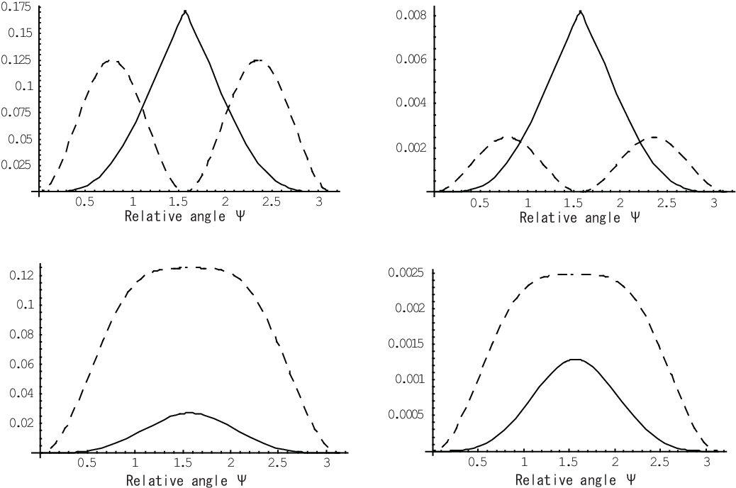
The general bound (81) should be compared to the bound previously obtained by the first approach, that is, Eq. (39). We plot these bounds both for θ=π\theta=\pi and θ=π/2\theta=\pi/2 (See Fig.2). Generally speaking, neither bound is tighter than the other. For θ=π/2\theta=\pi/2 and σ⁡(L𝐀/c)=1,or​ 10\sigma(L_{{\bf A}}/c)=1,{\rm{or}}\ 10, the previous bound (39) is tighter than the present bound (81) over all the relative angle Ψ\Psi. For θ=π\theta=\pi, the present bound does not vanish when Ψ=π/2\Psi=\pi/2; in fact, it reaches its peak, whereas the previous bound vanishes, which was the main motivation for this section.
Refer to caption
Figure 2: Comparison between the lower bound in Eq. (81) (Solid line) and that in Eq. (39) (dashed line). We set θ=π\theta=\pi and σ⁡(L𝐀/c)=1\sigma(L_{{\bf A}}/c)=1 in the upper left figure, and θ=π\theta=\pi and σ⁡(L𝐀/c)=10\sigma(L_{{\bf A}}/c)=10 in the upper right figure, and θ=π/2\theta=\pi/2 and σ⁡(L𝐀/c)=1\sigma(L_{{\bf A}}/c)=1 in the lower left figure, and θ=π/2\theta=\pi/2 and σ⁡(L𝐀/c)=10\sigma(L_{{\bf A}}/c)=10 in the lower right figure.

8 Concluding remarks

We investigated the limitations of the gate infidelity of implementing arbitrary single-qubit gates under arbitrary additive conservation laws. We obtained the two different lower bounds of the gate infidelity by using Robertson’s uncertainty relation. Both bounds were described by the variance of the conserved quantity and the parameters (θ,Ψ)(\theta,\Psi). The parameter Ψ\Psi is considered to be the relative angle between the axes of rotations on the Bloch sphere generated by the conserved quantity and the gate operation, which provides a geometrical understanding of the limitations in the three dimensional space. For the first bound (39), we show that it depends on the relative angle 2​γ2\gamma between the axis of rotations generated by the conserved quantity before and after the gate operation, in the Heisenberg picture. Both bounds are important because in general, neither bound is tighter than the other. Both bounds become zero if and only if θ=0\theta=0 or Ψ=0\Psi=0. This is expected because the conserved quantity LL commutes with the desired gate U𝐒U_{\mathbf{S}} only if θ=0\theta=0 or Ψ=0\Psi=0. Generally speaking, the limitations decrease as the variance of the conserved quantity increases, and given the variance and the parameters θ\theta and Ψ\Psi, the upper bound of both bounds provides the fundamental limitation for any implementation of the desired gate under the conservation law.

This research was partially supported by the SCOPE project of the MIC, the Grant-in-Aid for Scientific Research (B)17340021 of the JSPS, and the CREST project of the JST. J. G.-B.’s research was supported by the National Science Foundation.

Appendix A Ancilla in a mixed state

In this section, for completeness, we show that our results are not changed if we assume an arbitrary state ρ𝐀\rho_{{\bf A}}, which does not have to be a pure state, of the ancilla system as the initial state of the implementation ℰα{\cal E}_{\alpha}. In order to apply our previous treatment, we purify this state by introducing an auxiliary system 𝐁{\bf B}. The dimension of the auxiliary system 𝐁{\bf B} must be greater than or equal to that of the ancilla system so that the system 𝐁{\bf B} can provide the purification of any state of the ancilla system 𝐀{\bf A}. Suppose that |A′⟩|A^{\prime}\rangle is the purified state for the state ρ𝐀\rho_{{\bf A}} satisfying

Tr𝐁⁡[|A′⟩​⟨A′|]=ρ𝐀,\displaystyle\Tr_{{\bf B}}[|A^{\prime}\rangle\langle A^{\prime}|]=\rho_{{\bf A}}, (89)

where Tr𝐁\Tr_{{\bf B}} stands for the partial trace over the auxiliary system 𝐁{\bf B}. |A′⟩|A^{\prime}\rangle is a vector of the Hilbert space of the composite system 𝐀+𝐁{\bf A}+{\bf B}. This state can be considered as the initial state of the ancilla system if the ancilla system is extended to the original ancilla system 𝐀{\bf A} plus the auxiliary system 𝐁{\bf B}. In this case, the total system that we have is the composite system 𝐒+𝐀+𝐁{\bf S}+{\bf A}+{\bf B}, and the initial state of the implementation is given by ρ𝐒⊗|A′⟩​⟨A′|\rho_{{\bf S}}\otimes|A^{\prime}\rangle\langle A^{\prime}|. As the physical system is extended from the original system 𝐒+𝐀{\bf S}+{\bf A} to the system 𝐒+𝐀+𝐁{\bf S}+{\bf A}+{\bf B} to include the auxiliary system 𝐁{\bf B}, the time evolution operator of the implementation must also be extended to U′=U⊗I𝐁U^{\prime}=U\otimes I_{{\bf B}}, where I𝐁I_{\mathbf{B}} is the identity operator of 𝐁{\bf B}. Therefore the implementation is given by the trace-preserving quantum operation defined as

ℰα′​(ρ𝐒)=Tr𝐀+𝐁⁡[U′​(ρ𝐒⊗|A′⟩​⟨A′|)​U′⁣†]\displaystyle{\cal E}_{\alpha^{\prime}}(\rho_{{\bf S}})=\Tr_{{\bf A}+{\bf B}}\left[U^{\prime}(\rho_{{\bf S}}\otimes|A^{\prime}\rangle\langle A^{\prime}|)U^{\prime\dagger}\right] (90)

for any density operator ρ𝐒\rho_{{\bf S}} of the system 𝐒{\bf S}, where α′\alpha^{\prime} stands for the characterization of this quantum operation, α′=(U′,|A′⟩)\alpha^{\prime}=(U^{\prime},|A^{\prime}\rangle), and Tr𝐀+𝐁\Tr_{{\bf A}+{\bf B}} stands for the partial trace over the Hilbert space of 𝐀+𝐁{\bf A}+{\bf B}. The evolution operator U′U^{\prime} must obey the conservation law

[U′,L′]=0,\displaystyle[U^{\prime},L^{\prime}]=0, (91)

where L′=L𝐒⊗I𝐀⊗I𝐁+I𝐒⊗L𝐀⊗I𝐁L^{\prime}=L_{\mathbf{S}}\otimes I_{\mathbf{A}}\otimes I_{\mathbf{B}}+I_{\mathbf{S}}\otimes L_{{\bf A}}\otimes I_{\mathbf{B}}, which is the natural extension of the conserved quantity according to the above extension of the physical system. This conservation law is equivalent to the previous one (8)(\ref{eq:conservation}).

It is not difficult to verify that this extension does not change the calculations leading to the general bounds, that is, we can apply the same arguments as from Sec. 3 to Sec. 7 even in this case, and obtain

1−F​(ℰα′,U𝐒)2≥sin2⁡θ2​sin2⁡Ψ⁡(1−sin2⁡θ2​sin2⁡Ψ)1+σ​(L𝐀/c)2,\displaystyle 1-F({\mathcal{E}}_{\alpha^{\prime}},U_{{\bf S}})^{2}\geq\frac{\sin^{2}\frac{\theta}{2}\sin^{2}\Psi(1-\sin^{2}\frac{\theta}{2}\sin^{2}\Psi)}{1+\sigma(L_{{\bf A}}/c)^{2}}, (92)

and

1−F​(ℰα′,U𝐒)2≥1(1+1+σ​(L𝐀/c)2)2​[1−12​(‖v→‖+‖w→‖)]2.\displaystyle 1-F({\cal E}_{\alpha^{\prime}},U_{{\bf S}})^{2}\geq\frac{1}{\left(1+\sqrt{1+\sigma(L_{{\bf A}}/c)^{2}}\right)^{2}}\left[1-\frac{1}{2}(\|\vec{v}\|+\|\vec{w}\|)\right]^{2}. (93)

The only difficulty here is that the implementation ℰα′{\cal E}_{\alpha^{\prime}} appears different from the original one ℰα{\cal E}_{\alpha}. However, this problem is removed because the implementation ℰα′{\cal E}_{\alpha^{\prime}} is equivalent to the quantum operation characterized by the time evolution operator UU and arbitrary mixed states ρ𝐀\rho_{{\bf A}} of the ancilla system, that is,

ℰα′​(ρ𝐒)=Tr𝐀⁡[U⁡(ρ𝐒⊗ρ𝐀)​U]\displaystyle{\cal E}_{\alpha^{\prime}}(\rho_{{\bf S}})=\Tr_{{\bf A}}\left[U(\rho_{{\bf S}}\otimes\rho_{{\bf A}})U\right] (94)

for any density operator ρ𝐒\rho_{{\bf S}}. The proof is as follows. Since U′=U⊗I𝐁U^{\prime}=U\otimes I_{\mathbf{B}}, we have

ℰα′​(ρ𝐒)=Tr𝐀+𝐁⁡[U⊗I𝐁​(ρ𝐒⊗|A′⟩​⟨A′|)​U†⊗I𝐁].\displaystyle{\cal E}_{\alpha^{\prime}}(\rho_{{\bf S}})=\Tr_{{\bf A}+{\bf B}}\left[U\otimes I_{\mathbf{B}}(\rho_{{\bf S}}\otimes|A^{\prime}\rangle\langle A^{\prime}|)U^{\dagger}\otimes I_{\mathbf{B}}\right]. (95)

As |A′⟩​⟨A′||A^{\prime}\rangle\langle A^{\prime}| is the purification of the ρ𝐀\rho_{{\bf A}}, we see that

ℰα′​(ρ𝐒)\displaystyle{\cal E}_{\alpha^{\prime}}(\rho_{{\bf S}}) =\displaystyle= Tr𝐀⁡[U​Tr𝐁​[ρ𝐒⊗|A′⟩​⟨A′|]​U†]\displaystyle\Tr_{{\bf A}}\left[U\Tr_{{\bf B}}\left[\rho_{{\bf S}}\otimes|A^{\prime}\rangle\langle A^{\prime}|\right]U^{\dagger}\right] (96)
=\displaystyle= Tr𝐀⁡[U⁡(ρ𝐒⊗Tr𝐁⁡[|A′⟩​⟨A′|])​U†]\displaystyle\Tr_{{\bf A}}\left[U(\rho_{{\bf S}}\otimes\Tr_{{\bf B}}\left[|A^{\prime}\rangle\langle A^{\prime}|\right])U^{\dagger}\right] (97)
=\displaystyle= Tr𝐀⁡[U⁡(ρ𝐒⊗ρ𝐀)​U],\displaystyle\Tr_{{\bf A}}\left[U(\rho_{{\bf S}}\otimes\rho_{{\bf A}})U\right], (98)

which completes the proof. This proof has been already shown in Ref. [20].

We can then substitute Eq. (94) into Eq. (92) and (93) and obtain the general lower bounds, which are correct even if arbitrary initial states ρ𝐀\rho_{{\bf A}} of the ancilla system are assumed:

1−F​(ℰα,U𝐒)2≥sin2⁡θ2​sin2⁡Ψ⁡(1−sin2⁡θ2​sin2⁡Ψ)1+σ​(L𝐀/c)2,\displaystyle 1-F({\mathcal{E}}_{\alpha},U_{{\bf S}})^{2}\geq\frac{\sin^{2}\frac{\theta}{2}\sin^{2}\Psi(1-\sin^{2}\frac{\theta}{2}\sin^{2}\Psi)}{1+\sigma(L_{{\bf A}}/c)^{2}}, (99)

and

1−F​(ℰα,U𝐒)2≥1(1+1+σ​(L𝐀/c)2)2​[1−12​(‖v→‖+‖w→‖)]2,\displaystyle 1-F({\cal E}_{\alpha},U_{{\bf S}})^{2}\geq\frac{1}{\left(1+\sqrt{1+\sigma(L_{{\bf A}}/c)^{2}}\right)^{2}}\left[1-\frac{1}{2}(\|\vec{v}\|+\|\vec{w}\|)\right]^{2}, (100)

where the quantum operation ℰα{\cal E}_{\alpha} is defined as

ℰα​(ρ𝐒)=Tr𝐀⁡[U⁡(ρ𝐒⊗ρ𝐀)​U]\displaystyle{\cal E}_{\alpha}(\rho_{{\bf S}})=\Tr_{{\bf A}}\left[U(\rho_{{\bf S}}\otimes\rho_{{\bf A}})U\right] (101)

for any state ρ𝐒\rho_{{\bf S}}.

References

References

  • [1] M. A. Nielsen and I. L. Chuang, Quantum Computation and Quantum Information (Cambridge University Press, Cambridge, 2000).
  • [2] J. P. Barnes and W. S. Warren, Phys. Rev. A 60, 4363 (1999).
  • [3] S. J. van Enk and H. J. Kimble, Quantum Inf. Comput. 2, 1 (2002).
  • [4] J. Gea-Banacloche, Phys. Rev. A 65, 022308 (2002).
  • [5] J. Gea-Banacloche, Phys. Rev. Lett. 89, 022308 (2002).
  • [6] J. Gea-Banacloche and L. B. Kish, Fluctuation and Noise Letters 3, C3 (2003).
  • [7] J. Gea-Banacloche and L. B. Kish, Proc. IEEE 93, 1858 (2005).
  • [8] A. Silberfarb and I. H. Deutsch, Phys. Rev. A 69, 042308 (2004).
  • [9] F. Xue, S. X. Yu, and C. P. Sun, Phys. Rev. A 73, 013403 (2006).
  • [10] W. M. Itano, Phys. Rev. A 68, 046301 (2003).
  • [11] S. J. van Enk and H. J. Kimble, Phys. Rev. A 68, 046302 (2003).
  • [12] J. Gea-Banacloche, Phys. Rev. A 68, 046303 (2003).
  • [13] M. Ozawa, Phys. Rev. Lett. 89, 057902 (2002).
  • [14] M. Ozawa, Phys. Rev. Lett. 88, 050402 (2002).
  • [15] M. Ozawa, Int. J. Quant. Inf. 1, 569 (2003).
  • [16] M. Ozawa, in Proceedings of the Sixth International Conference on Quantum Communication, Measurement and Computing, edited by J. H. Shappiro and O. Hirota (Rinton Press, Princeton, 2003), pp. 175–180.
  • [17] E. P. Wigner, Z. Phys. 133, 101 (1952).
  • [18] H. Araki and M. M. Yanase, Phys. Rev. 120, 622 (1960).
  • [19] M. M. Yanase, Phys. Rev. 123, 666 (1961).
  • [20] T. Karasawa and M. Ozawa, Phys. Rev. A 75, 032324 (2007).
  • [21] J. Gea-Banacloche and M. Ozawa, J. Opt. B: Quantum Semiclass. Opt. 7, S326 (2005).
  • [22] J. Gea-Banacloche and M. Ozawa, Phys. Rev. A 74, 060301(R) (2006).
  • [23] M. A. Nielsen and I. L. Chuang, Phys. Rev. Lett. 79, 321 (1997).
  • [24] M. Hillery, M. Ziman and V. Buč ek, Phys. Rev. A 73, 022345 (2006).
  • [25] E. Jaynes and F. W. Cummings, Proc. IEEE 51, 89 (1963).
  • [26] H. P. Robertson, Phys. Rev. 34, 163 (1929).