Non-Gibrat’s law in the middle scale region
Abstract
By using numerical simulation, we confirm that Takayasu–Sato–Takayasu (TST) model which leads Pareto’s law satisfies the detailed balance under Gibrat’s law. In the simulation, we take an exponential tent-shaped function as the growth rate distribution. We also numerically confirm the reflection law equivalent to the equation which gives the Pareto index in TST model. Moreover, we extend the model modifying the stochastic coefficient under a Non-Gibrat’s law. In this model, the detailed balance is also numerically observed. The resultant pdf is power-law in the large scale Gibrat’s law region, and is the log-normal distribution in the middle scale Non-Gibrat’s one. These are accurately confirmed in the numerical simulation.
PACS code : 89.65.Gh
1 Introduction
Recent developments of computer technology enable vast quantities of economic data to be analyzed. As one of remarkable examples, Fujiwara et al. [1] find that Pareto’s law [2]
| (1) |
can be derived from the law of detailed balance
| (2) |
and Gibrat’s law [3]
| (3) |
which are observed in massive amounts of economic data. Here is wealth, income, profits, assets, sales, the number of employees and so forth, and , are two successive those. is a joint probability density function (pdf), and is a conditional pdf of the growth rate .
The Pareto’s law (1) is not observed below some threshold [3, 4], because the Gibrat’s law (3) does not hold in the middle scale region [5, 6, 7]. In Ref. [8], we show that the detailed balance (2) and a Non-Gibrat’s law
| (4) | |||||
| (5) |
lead the log-normal distribution in the middle scale region as follows:
| (6) |
The Non-Gibrat’s law means a statistical dependence of the growth rate distribution on the past value in the middle scale region. In the derivation, we employ the approximation (4) observed in profits data of Japanese firms[9], and find that the expression of (5) is unique under the detailed balance. Employing such empirical data, we confirm that the resultant distribution (6) fits with data in the large scale Pareto’s law region and those in the middle scale log-normal region consistently. The parameters are estimated as follows: for , for ,11 1 Here, a constant parameter takes different values in two regions. This is not an exact procedure. However, for firms which are in the large scale region in both years ( and ) or in the middle scale one ( and ), this procedure is exact. In the database, most firms stay in the same region. This parameterization is, therefore, approximately valid for describing the probability density function . This is empirically confirmed in Ref. [8]. thousand yen and thousand yen [8].
These data analyses are sufficiently rigorous, but at the same time are restricted in the finite period and category, because it is not easy to procure exhaustive data. If we build a model based on the detailed balance and (Non-)Gibrat’s law, various economic situations can be simulated. This might make the reason clear why the parameters take the empirical values. Furthermore, we can study assets or sales data of firms which are difficult to obtain. In this paper, we will propose the simulation model based on the observation of economic data.
2 TST model
Firstly, we identify the model which leads Pareto’s law based on the detailed balance and Gibrat’s law in the large scale region. One of the simplest and powerful candidates is Takayasu–Sato–Takayasu (TST) model [10], which is given by the Langevin equation
| (7) |
where is a non-negative stochastic coefficient and is a random additive noise. They show that the conditions
| (8) |
are necessary and sufficient for the power-law (1), the index of which is given by the equation
| (9) |
Here denotes an average over realizations.
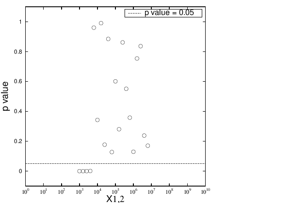
In order to claim that this model is consistent with the empirical observation, the detailed balance and Gibrat’s law must be satisfied. From Eq. (7), Gibrat’s law is hold in the region where a noise is negligible. The result in Ref. [1] suggests, therefore, that there is the detailed balance in TST model which leads Pareto’s law. In the numerical simulation, we adopt the distribution of and to be Eqs. (4)–(5) with and Weibull distribution: , respectively. The typical scatter plot of the simulation is shown in Fig. 2, where we take , , , and . To check the validity of the detailed balance, we take the one-dimensional Kolmogorov-Smirnov (K-S) test. We compare the distribution sample for with another sample for with by making the null hypothesis that these two samples are taken from a same parent distribution. Each value is shown in Fig. 2. The null hypothesis is not rejected in 5 significance level in the region where the noise is negligible. We recognize that the detailed balance is observed in the region. The lower bound of the region is denoted by , above which Pareto’s law is observed (Fig. 4).



In addition, we also confirm the reflection law derived in Ref. [1]. In this simulation, from Eqs.(4) and (5) with , the reflection law is reduced to 22 2 This equation is also confirmed empirically in profits data of Japanese firms [8].
| (10) |
which is equivalent to the condition (9). We observe this reflection law in various (Fig. 4). From these results, TST model is appropriate satisfying the detailed balance under the Gibrat’s law.
3 Simulation under Non-Gibrat’s law
If the detailed balance is satisfied even under a Non-Gibrat’s law in the simulation, the log-normal distribution must be reduced in the middle scale region [8]. In a stochastic method, this scheme is not obvious analytically. Because a non-negative stochastic coefficient in Eq. (7) must be modified as under the Non-Gibrat’s law. This extension exceeds the analytical framework of TST model. However, we can examine the scheme numerically.
In the simulation, is introduced satisfying . We adopt the distribution of to be Eqs. (4)–(5) with for (Gibrat’s law), for (Non-Gibrat’s law) and for keeping continuously (Fig. 6). The last parameterization is imposed to exclude immoderate slopes of growth rate distributions. As the Non-Gibrat’s region in the middle scale, we observe the region .


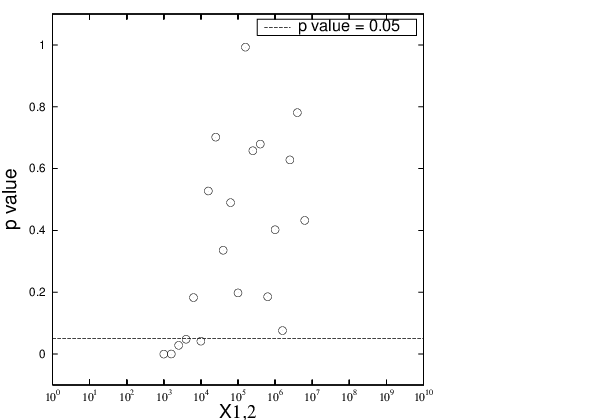
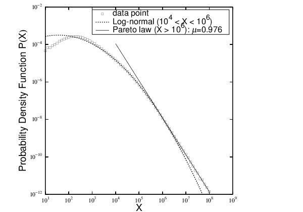
The typical scatter plot of the simulation is shown in Fig. 6, where we take , , , , and . To check the validity of the detailed balance, we take the same K-S test in the previous section. The result is shown in Fig. 8. The detailed balance is confirmed not only in the Gibrat’s large scale region () but also in the Non-Gibrat’s middle scale one (). The resultant pdf of is shown in Fig. 8, where the log-normal distribution in the middle scale region is observed in addition to Pareto’s law in the large scale one. To confirm the validity of the log-normal distribution, we check the correlation between the parameter inputted in the simulation and that estimated by fitting the pdf in the Non-Gibrat’s region (denoted by ). The result is shown in Fig. 10 for the case , , , and and in Fig. 10 for the case , , , and for example. The correlation is very high. Consequently, this simulation model is also appropriate satisfying the detailed balance even under the Non-Gibrat’s law.


4 Summary and future problems
In this study, by using numerical simulation, we confirm that TST model which leads Pareto’s law satisfies the detailed balance under Gibrat’s law. In the simulation, we take an exponential tent-shaped function as the growth rate distribution. We also numerically confirm the reflection law [1] equivalent to the equation which gives the Pareto index in TST model. Moreover, we extend the model modifying the stochastic coefficient under a Non-Gibrat’s law. In this model, the detailed balance is also observed. The resultant pdf is power-law in the large scale Gibrat’s law region, and is the log-normal distribution in the middle scale Non-Gibrat’s one. These are accurately confirmed in the numerical simulation.
In this simulation, we employ the Non-Gibrat’s law (5) that the probability of the positive growth decreases and that of the negative growth increases symmetrically as the classification of increases (Figs. 6, 12). This is uniquely derived from the exponential tent-shaped form (4) observed in Japanese profits data [8]. On the other hand, as for sales or assets of firms, it is reported that the probability of the positive and negative growth decrease simultaneously as the classification of increases (Fig. 12). This difference is thought to be caused by the form of the exponential tent-shaped growth rate distribution. Eq. (4) is rewritten by using the pdf for as follows:
| (11) |
For sales or assets of firms, these linear approximations are not used to express the growth rate distribution with the curvature [1].


In order to count the curvature, we add a second order term with respect to :
| (12) |
In terms of , these are expressed as
| (13) |
In this case, the detailed balance (2) is reduced to be
| (14) |
for . By setting after differentiating Eq. (14) with respect to , differential equations are obtained. The solutions are uniquely fixed as
| (15) | |||||
| (16) | |||||
| (17) | |||||
| (18) | |||||
| (19) |
with . Same solutions are obtained for . Here we set the parameters as follows: for (Gibrat’s law), and for (Non-Gibrat’s law) because are constants.
As an index of increase and decrease of the probability of the growth rate, we examine the differential coefficient at the origin: . We are, therefore, interested in the increase and decrease of in the middle scale region. In the case for example, the results are shown in Figs. 14 and 14 using the notation , . Consequently the solution, that the probability of the positive and negative growth decrease simultaneously as the classification of increases, exists in following parameter regions:
| (20) | |||||
| (21) | |||||
| (22) |
In any case, have no first order term and the negative second order term with respect to . Not only parameter but also is necessary for the solution. We will apply the simulation to this analysis in the next work.


As other application of the simulation, the detailed balance is expected to be extended to the detailed quasi-balance [11] observed in the assessed value of land in Japan [12, 13]. If these applications are studied adequately, we can manage the risk of these quantities by using knowledge of this method.
Acknowledgements
We would like to thank the Yukawa Institute for Theoretical Physics at Kyoto University, where this work was initiated during the YITP-W-07-16 on “Econophysics III–Physical Approach to Social and Economic Phenomena–”, and especially to Dr Y. Soejima for the important comments about our work. Thanks are also due to Dr. A. Sato for a lot of useful discussions. This work was supported in part by a Grant–in–Aid for Scientific Research (C) (No. 20510147) from the Ministry of Education, Culture, Sports, Science and Technology, Japan.
References
- [1]
Y. Fujiwara, W. Souma, H. Aoyama, T. Kaizoji and M. Aoki,
Physica A321 (2003), 59.
Y. Fujiwara, C.D. Guilmi, H. Aoyama, M. Gallegati and W. Souma, Physica A335 (2004), 197. - [2] V. Pareto, Cours d’Economique Politique (Macmillan, London, 1897).
- [3] R. Gibrat, Les inegalites economiques (Sirey, Paris, 1932).
- [4]
W.W. Badger, in: B.J. West (Ed.),
Mathematical Models as a Tool for the Social Science
(Gordon and Breach, New York, 1980), p. 87.
E.W. Montrll, M.F. Shlesinger, J. Stat. Phys. 32 (1983), 209. - [5] M.H.R. Stanley, L.A.N. Amaral, S.V. Buldyrev, S. Havlin, H. Leschhorn, P. Maass, M.A. Salinger, H.E. Stanley, Nature 379 (1996), 804.
- [6] H. Takayasu, M. Takayasu, M.P. Okazaki, K. Marumo, T. Shimizu, cond-mat/0008057, in: M.M. Novak (Ed.), Paradigms of Complexity (World Scientific, 2000), p. 243.
- [7]
H. Aoyama,
Ninth Annual Workshop on Economic Heterogeneous Interacting Agents (WEHIA 2004).
H. Aoyama, Y. Fujiwara, W. Souma, The Physical Society of Japan 2004 Autumn Meeting. - [8] A. Ishikawa, Physica A367 (2006), 425; Physica A383/1 (2007), 79.
- [9] TOKYO SHOKO RESEARCH, LTD., http://www.tsr-net.co.jp/.
- [10] H. Takayasu, A. Sato and M. Takayasu, Phys. Rev. Lett. 79 (1997), 966.
- [11] A. Ishikawa, Physica A371 (2006), 525.
- [12]
T. Kaizoji, Physica A326 (2003), 256.
T. Kaizoji and M. Kaizoji, Physica A344 (2004), 138. - [13] The Ministry of Land, Infrastructure and Transport Government of Japan’s World-Wide Web site, http://nlftp.mlit.go.jp/ksj/.