Interference Alignment for Line-of-Sight Channels
Abstract
The fully connected -user interference channel is studied in a multipath environment with bandwidth . We show that when each link consists of physical paths, the total spectral efficiency can grow linearly with . This result holds not merely in the limit of large transmit power , but for any fixed , and is therefore a stronger characterization than degrees of freedom. It is achieved via a form of interference alignment in the time domain. A caveat of this result is that must grow with , a phenomenon we refer to as bandwidth scaling. Our insight comes from examining channels with single path links (), which we refer to as line-of-sight (LOS) links. For such channels we build a time-indexed interference graph and associate the communication problem with finding its maximal independent set. This graph has a stationarity property that we exploit to solve the problem efficiently via dynamic programming. Additionally, the interference graph enables us to demonstrate the necessity of bandwidth scaling for any scheme operating over LOS interference channels. Bandwidth scaling is then shown to also be a necessary ingredient for interference alignment in the -user interference channel.
1 Introduction
The problem of communicating efficiently in wireless adhoc networks has received much attention of late, the focus being on how to deal with interference in a shared medium. Traditional approaches based on orthogonalizing users (eg. TDMA or FDMA) or reusing the spectrum (eg. CDMA, certain modes of 802.11) suffer from poor spectral efficiency. In particular as the number of users in the system grows, the spectral efficiency of each link vanishes. More recent approaches include using multi-hop [1], distributed MIMO [2], [3], and interference alignment [4], [5], [6]. This work belongs to the latter category. Interference alignment is a technique that uses appropriate precoding to compact interfering signals into small dimensional subspaces at each receiver. At the same time, the subspace occupied by the data remains linearly independent of the interference. It was first applied to a multiple MIMO base station problem in [4] and shown to be capable of achieving multiplexing gains distinctly greater than those achievable using conventional signalling schemes. The technique was then extended in [6] to show that there were exactly degrees of freedom in the MIMO X channel (two MIMO transmitters each desiring to send data to two MIMO receivers) with antennas at each transceiver. Following this, a more sophisticated interference alignment technique was developed in [5] for the -user interference channel with an infinite number of independently faded sub-channels, and used to demonstrate that contrary to conventional wisdom, the total degrees of freedom of the channel is .
Whilst the last approach demonstrates the potential benefits that interference alignment techniques can provide, it suffers from a number of limitations. Perhaps the foremost is that whilst a degrees of freedom characterization is useful in the high limit, it may not be meaningful at moderate ’s. This stems from the fact that degrees of freedom characterizes the asymptotic slope of the spectral efficiency curve and not its actual value. In particular, it is unclear whether at any fixed the total spectral efficiency of the system is increasing in proportion to , or increasing at all. The point here is that [5] does not contain a scaling law result the likes of [1] and [2], that is, it does not tell us what happens to the system capacity as more users enter the fray. We address this question by constructing a communication scheme that achieves a scaling of system capacity arbitrarily close to linear.
There is another key limitation. It is natural to interpret the parallel channels used in the interference alignment scheme of [5] as corresponding to sub-channels in the frequency domain. This is due to various difficulties associated with realizing the scheme over independently faded parallel channels in time, most notably the very rapid and accurate channel measurement that must take place, and the substantial delay incurred. But in order for a large number of frequency channels to undergo independent fading, significant scattering/multipath is required.
In this work we examine the -user interference channel with limited multipath. We start by assuming each of the links consists only of a single physical path with complex gain and delay seconds. This model is a good representation for a line-of-sight (LOS) channel. Following this we generalize to the case where each link consists of physical paths. We illustrate a simple and elegant representation of interference alignment in the time domain, in terms of aligning symbols on a time-indexed interference graph. This interference graph proves to be an extremely useful tool for both conceptualizing and solving various problems relating to interference in LOS channels. We identify the problem of communicating on the LOS interference channel with the problem of finding a maximal independent set in the interference graph, and show how this problem can be solved efficiently using dynamic programming principles. The simplicity of this approach makes it quite versatile and potentially capable of being extended to tackle a variety of related problems.
For the remainder of this work power spectral density () is used in place of signal-to-noise ratio, as we will later wish to compare schemes that use different bandwidths. Depending on the link delays, it may be possible to achieve a spectral efficiency as high as bps/Hz for each user , regardless of the number of interferers. This is exactly half the spectral efficiency achievable in the absence of interference. We characterize the precise channel conditions for which this is possible and show that they occur in at least 1/16 of all scenarios for the -user interference channel.
This of course, says little about the typical gains one can expect by aligning interference in the time domain. To address this question, we treat the link delays as independent and uniformly distributed random variables in , where is the delay-spread of the channel. Previous work such as [4], [5], [6] has focused on degrees of freedom as a metric for performance, which is a measure of the scaling of spectral efficiency with when the power spectral density is large. We focus on the scaling of spectral efficiency with when the number of users is large. The main result of this work is the construction of a communication scheme that achieves a spectral efficiency arbitrarily close to for each user as . Thus our result characterizes the best possible scaling of spectral efficiency with for any fixed , as compared with [4], [5], [6], where the best possible scaling of spectral efficiency with , for any fixed , is characterized. In this sense, our characterization has a similar flavor to characterizations of scaling laws for wireless adhoc networks such as [1], [2], however, our scheme requires no cooperation between users.
A caveat of our result is that the bandwidth must scale sufficiently with . Interpreting the parallel channel model of [5] in the frequency domain, one sees that the bandwidth there must also scale with . Interestingly enough, the bandwidth scaling required for our scheme is essentially the same as that required in [5], namely . However, whereas the scheme in [5] requires coding over blocks of length , which creates significant encoding and decoding complexity issues as well as substantial delay, our scheme requires no block coding, and consequently does not incur any delay or suffer from complexity issues.
Essentially, in order to align interference into a small dimensional subspace and keep it linearly independent of the data subspace, a high degree of resolvability of the received signals is required. We establish this concretely for the LOS channel in the context of the interference graph, showing that if the bandwidth scales sub-linearly with , then the total spectral efficiency of the system (the sum of all users spectral efficiencies) will scale sublinearly, and hence almost all of the users will witness vanishing spectral efficiencies as increases.
This suggests that the greatest performance gains can be reaped in systems with large delay spreads. Perhaps the best example of such a system is the backbone of a mesh network, used to wirelessly connect rural areas. Such systems are well approximated by a LOS model, have large delay spreads, and are relatively static, making channel measurement simpler and more accurate.
The structuring of the rest of the paper is as follows. In section 2 we describe the model of the -user LOS interference channel. Section 3 provides a summary of the main result concerning the achievability of non-vanishing spectral efficiencies as the number of users grows. The time-indexed interference graph is introduced in section 4. In the same section we present an algorithm for optimizing the spectral efficiency efficiently via dynamic programming. We also address the questions of bandwidth scaling, and of characterizing the class of channels for which the spectral efficiency can reach its maximum value. In section 5 we present our construction that establishes the main result. Following this, in section 6, we establish the relationship between time and frequency domain interference alignment techniques. Section 7 contains further discussion, extensions and open problems.
2 Model
We consider the -user interference channel in which there are transmitters and receivers. Transmitter wishes to send data to receiver but its transmission constitutes interference at all other receivers. We often refer to each tx-rx pair as a user. There are thus links in total, direct links and cross-links. Each link consists of a single physical path. Denote the gain and delay (in seconds) of the link between transmitter and receiver by and , respectively. We assume the and are fixed for the duration of communication. Denote the signal transmitter sends by . Then the baseband signal at the th receiver is
where the are i.i.d. white noise processes with power spectral density Watts/Hz. Denote the carrier frequency and the bandwidth that the signals are constrained to lie in by Hz. Assuming the use of ideal sinc pulses, the passband signal after sampling is given by
where the are i.i.d. . We use the following conventional approximation for the pulse,
see page 27 of [7]. Let denote the integer round-off of the real number . This leads to
In a wireless model one typically makes an assumption about the statistics of the channel. For example, in a channel with ISI, the tap coefficients are often modeled as i.i.d. Rayleigh random variables. In models where there is a dominant path, Rician random variables are used instead. Likewise in this work we make a statistical assumption on the channel, but limit this statistical assumption only to the link delays, taking the to be i.i.d. uniform in , where denotes the delay-spread of the channel in seconds. This means that if we define to be one plus the integer round off of , the are i.i.d. uniform in . No assumption is made on the link gains , other than they all being non-zero.
We refer to this as the -user line-of-sight (LOS) interference channel, as this is the most common scenario giving rise to such a model.
There is a straightforward extension of this model to the case where each link consists of physical paths, such that the th received signal is
Here and are the complex gain and delay of the th physical path between transmitter and receiver . This leads to the following generalization of the passband model after sampling
The natural extension of our statistical assumption for the LOS channel is to treat the delays as i.i.d. uniform in . In doing so we are assuming independent delays not just across physical paths of different links, but also across the physical paths corresponding to the same link.
We refer to this as the -user -path interference channel.
3 Preview of Main Result
Theorem 3.1.
For any , there exists a communication scheme on the -user LOS interference channel such that if , the expected spectral efficiency of user tends to
| (1) |
as .
Section 5 is devoted to proving this result. Here the expectation of spectral efficiency is taken over the random direct delays . Roughly speaking this result says that as scales, it is possible for each user to communicate at a spectral efficiency arbitrarily close to , so long as the bandwidth scales as fast as . In other words, communication at spectral efficiencies that vanish arbitrarily slowly with is possible if the bandwidth scales sufficiently. In this result, and throughout this work, we assume that all cross delays for are known at all transmitters and receivers. This result is of a similar nature to the scaling laws of [2], in that we show the growth of system capacity with the number of users is arbitrarily close to linear. Unfortunately, as is the case in [5], the required bandwidth scaling is great. A result presented later on (theorem 4.2) addresses the question of whether bandwidth scaling is necessary.
For the case where each link consists of physical paths we have the following generalization.
Theorem 3.2.
For any , there exists a communication scheme on the -user -path interference channel such that if , the expected spectral efficiency of user tends to
| (2) |
as .
As is evident from the statement of the theorem, there is a tradeoff between the number of physical paths per link and the bandwidth scaling required. Again, the question of whether this bandwidth scaling is necessary is addressed in a result presented later on.
4 The Interference Graph
The key insight leading to theorem 3.1 comes from formulating the communication problem in a graph theoretical setting. We start with an example. Consider a -user LOS interference channel where the direct links are all zero, i.e. , and , and the cross-links are say, , , , , , . Choose a length for the communication block. Create a directed graph as follows. Let the vertex set be
The vertex represents the th time slot for the th transmitter. Form the edge set as follows. Add a directed edge starting from vertex and ending at vertex . This represents the fact that, owing to a delay of 3 time slots, a transmission during time slot 0 by transmitter 1 arrives at receiver 2 during time slot 3. Also add a directed edge starting from and ending at . This represents the fact that, owing to a delay of 1 time slot, a transmission during time slot 0 by transmitter 1 arrives at receiver 3 during time slot 1. Likewise add directed edges and from vertex to and , respectively, and directed edges and from vertex to and , respectively. This set of six edges encapsulates all of the interference generated by transmissions during time slot 0. As the channel is time-invariant the same interference structure applies for later time slots. Thus for each add a directed edge from to , provided , a directed edge from to , provided , a directed edge from to , provided , etc… See figure 1 for an illustration.

In this example all direct delays were zero, whereas in general this is not the case. However as each transmitter can merely offset it’s transmitted sequence by , we can effectively assume without loss of generality that . More concretely we define the normalized cross-delays
Note that , that is, it is possible for to be negative. At this point one may wonder why the interference graph need be directed, since the feasibility of a given transmit pattern is independent of edge direction. The answer is it need not be, but we define it as such to aid in conceptualizing the problem.

In general we have
Definition 4.1.
The time-indexed interference graph (or simply interference graph for short) of length associated with the -user LOS interference channel with normalized cross-delays , is the directed graph where
with edge stemming from vertex and ending at vertex .
This graph has vertices and approximately edges. As a transmission during time slot is interfered with by one time slot at each other user, and itself interferes with one time slot at each other user, each vertex has both in-degree and out-degree . To reduce the notational burden, we often refer to the graph simply as , where the parameters of the interference graph are implicit.
One can similarly define a time-indexed interference graph for the -path interference channel, but in the interest of brevity and clarity we do not discuss it here.
A transmit pattern is a subset of time slots during which data symbols are sent, one data symbol being sent per time slot. A transmit pattern is called feasible if each data symbol is received during a time slot that contains no interference from other transmissions. Thus a feasible transmit pattern corresponds to an independent set on the interference graph. Occasionally we will drop the adjective “feasible” when it is clear that the transmit pattern in question is such. As each data symbol arriving at receiver during a time slot containing no interfering symbol, is capable of conveying bps/Hz, user ’s spectral efficiency will be
where is the number of vertices in that are in the independent set. Let us assume for the meantime that for all . Then the total spectral efficiency is directly proportional to the size of the independent set. Thus the problem of designing a communication scheme to maximize total spectral efficiency reduces to finding the maximal independent set of the interference graph. Denote the size of the maximal independent set of a graph (called the independence number) by . Then the maximum total spectral efficiency for a graph is
For the preceding example, the maximal independent set is illustrated in figure 2. Whenever an independent set contains two vertices that possess a mutual neighbor, the interference generated by these two transmissions aligns at the mutual neighboring vertex. This is interference alignment in the time domain. For the example in figure 2, the neighbors of each unshaded vertex are all shaded, that is, data transmissions occur at all neighbors of an unshaded vertex. This is not always the case. Suppose we use a TDMA based communication scheme where user 1 transmits on consecutive time slots for a long period whilst users 2 and 3 remain silent. Then after a small guard interval user 2 transmits on consecutive time slots whilst users 1 and 3 remain silent. Finally user 3 transmits, and then back to user 1 and so on. In this round robin scheme, each unshaded vertex is connected to only a single shaded one and no interference alignment occurs.
The problem of finding the maximal independent set is a well-known NP-hard problem, meaning that for an arbitrary graph, there is no known algorithm capable of solving the problem in time sub-exponential in the number of vertices. Knowing this it may appear that finding an optimal transmit pattern requires a computation time that is exponential in the block length , however the interference graph is not an arbitrary graph. In particular it is stationary in the sense that, ignoring boundary effects, the structure of the graph is invariant to time shifts. In the next section we present an algorithm that exploits this property to find the maximum independent set in linear time. More generally, when the link gains are arbitrary the algorithm solves the problem of finding an independent set that maximizes spectral efficiency. We refer to this set as the optimal independent set.
4.1 Finding the maximal independent set efficiently
In this section we concentrate on the LOS channel, but the ideas can be extended to the -path channel. Given an interference graph we now illustrate how dynamic programming principles can be employed to compute the maximal independent set efficiently. Let each vertex with if is included in the transmit pattern, that is, if a data symbol is transmitted by user during time slot , and otherwise. There is a slight abuse of notation here as we have used to represent both an element of the vertex set and an indicator function for whether or not a data symbol is transmitted by transmitter during time slot .

Concretely stated, the optimization problem we will solve is
| (3) |
where . This is the problem of finding the optimal independent set. This cost is just the sum of the spectral efficiencies of the users weighted by the number of data symbols they send. We use a negative sign so as to justify the description of this metric as a cost, i.e. something we are trying to minimize. In the event that all direct gains are equal, is independent of and the problem reduces to finding the maximal independent set of .
To solve this problem efficiently, we start by defining
This is the length of the longest edge that connects a vertex at a time , to a vertex belonging to user for time . When all the are positive, simply represents the longest edge stemming from user . In the example of figure 1, , and . When some of the are negative, represents the longest edge connecting user to another user in the forward time direction. Thus the total amount of memory in the system is . If this seems somewhat contrived, recall that although the interference graph is a directed graph, it need not be defined as such, as the effect of vertex causing interference at vertex is identical to the effect of vertex causing interference at vertex . What matters for the dynamic programming formulation in this section, is not whether is causing interference with or vice versa, but whether , or . In our algorithm we move through vertices in order of increasing time . The state of the system at time is defined by those vertices at times that are connected to vertices at times .
More precisely, define the state vector at time to be
| (4) |
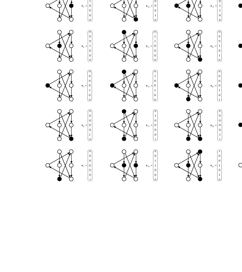
This is the collection of all vertices at times , that interfere with, or are interfered with by vertices at times . Figure 3 illustrates which vertices are included in the state vector. As each takes on one of two values, the state space consists of at most possible states. Some states may be infeasible because two of their vertices are connected by an edge. Thus define the state space as the space of all feasible states
with each . Each state in corresponds to an independent set in the subgraph made up of vertices in . Thus there are typically far fewer than states. A second example is given in figures 4 and 5. In this example there are a total of 28 states as shown in figure 5.
For notational convenience we label the elements of as such
Denote the set of feasible state transitions from to by

With the state space clearly defined, it is straightforward to derive the actual algorithm, which is akin to the Viterbi algorithm. It begins by initializing the costs to zero, that is
for all . Each iteration of the algorithm involves finding the minimum cost path entering each state. At times compute
for each , which is the minimum cost state at time from which we can transition into state at time . Then compute
for each , which is the minimum cost of a path that ends up at state at time . When time is finally reached, compute
which is the optimal termination state. The optimal independent set is then found by working backwards. Start by setting the th column of vertices according to . That is, set for . Then set the th column according to , that is, set for . Continue by setting , etc…
We now briefly examine the complexity of this algorithm. As the state space consists of all independent sets of a subgraph defined by vertices, given a set of delays , it takes time steps to enumerate. Once this is done, the algorithm takes time steps to solve problem (3). Roughly speaking, , and . Thus the algorithm takes
time steps to compute the optimal independent set.
As the state space defined in equation 4 is finite, for large the optimal independent set will have a periodic form with period less than or equal to the number of states . Thus, if there is no restriction on how large can be, once the period of the maximal independent set is found, we can simply set equal to it, without compromising optimality. In this case, the entire problem can be solved in
time steps.
4.2 Bandwidth scaling
Theorem 3.1 shows that if the bandwidth scales sufficiently quickly with , the spectral efficiency per user can be made to vanish arbitrarily slowly. A natural question to ask is whether it is necessary for the bandwidth to scale with , in order for this desirable property to hold. The following converse result establishes that this is indeed the case.
Theorem 4.2.
If the bandwidth scales sufficiently slowly with such that
then
| (5) |
with probability one.
As the total spectral efficiency
theorem 4.2 implies
which is equivalent to for almost all users .
Roughly speaking the above result says that if the bandwidth scales slower than , then the spectral efficiency resulting from any feasible transmit pattern will vanish as . Note there is a gap between this converse result and the achievability result of theorem 3.1. Theorem 3.1 demonstrates that it is sufficient for the bandwidth to scale like , but theorem 4.2 shows that it is necessary for the bandwidth to scale only as fast as . This establishes that the slowest possible bandwidth scaling lies somewhere between and . It is unclear, which if any of these bounds is tight.
Proof.
Remove those edges that connect vertices of different time slots in the interference graph, for . This provides an upper bound on the independence number. Now consider a single column of this graph in isolation. For any pair of vertices in , there exists an edge connecting them independently with probability (probability for each of the two possible directions). Thus the graph consisting of vertices and the random subset of edges connecting them, is precisely the Erdős-Rényi graph . A well known result (see for example [8]) is that
with probability one. Hence the independence number of satisfies
As is directly proportional to , if then the same limit applies for and
Now as the independence number of the interference graph satisfies , equation (5) follows. ∎
4.3 When is the maximal independent set maximal?
We now turn to the problem of analysis. Ideally we would like a simple characterization of the size of the maximal independent set in terms of the parameters of the system, , , and the normalized cross-delays . It is unclear if such a characterization exists. Instead we present two results. The first characterizes when the independence number is equal to its maximum possible value, and shows how the maximal independent set can be found almost instantly in this event. The second, which is theorem 3.1, demonstrates that surprisingly large independent sets exist on average, when both the number of users and the bandwidth are sufficiently high. In this section we present the former result, in the next section we present the latter. What we will be revealed in this section is that the problem of determining whether or not the independence number is equal to its maximum possible value, is a group theoretic one.
We assume in this section that the direct gains are all equal so that the optimal independent set is equivalent to the maximal independent set. Owing to the absence of some edges, the boundary of the interference graph has a slightly different structure than it’s interior. In order to circumvent this problem, we let so that these boundary effects are negligible.
Definition 4.3.
The independence rate of sequence of interference graphs
is
We write for short. Start with the following observation.
Lemma 4.4.
For any number of users and any channel
This means that for large we can only include at most half the vertices of the interference graph in any feasible transmit pattern. We now ask, when is the independence rate exactly equal to ? The following result succinctly answers this question for . Define
If , define to be the exponent of 2 in the prime factorization of , that is where represents the rest of the prime factorization. If then define . Similarly if , define to be the exponent of 2 in the prime factorization , i.e. . If then define .
Theorem 4.5.
if and only if , and , in which case there are exactly feasible transmit patterns achieving it.
To clarify, if for example both and , then the above conditions are not satisfied and . This theorem provides a necessary and sufficient condition such that all users can transmit half the time without interfering with one another. The most probable way this condition can be met is if is an odd number, and and are all even numbers. Each of these events roughly occurs independently with probability , hence the probability all four occur simultaneously is . Thus with probability there exists a feasible transmit pattern enabling all users to transmit half the time without interfering with one another. There are of course other ways in which our condition can be met, for example, if is even, but not a multiple of 4, and and are all multiples of 4, however this, and all other configurations satisfying the condition of theorem 4.5 likely occur with probability much less than . The proof of theorem 4.5 is given in the appendix.
Example 4.6.
For the channel in figure 11, we have and . This means , so a feasible transmit pattern achieving independence number exists. As there are only two feasible transmit patterns: the first is shown in the figure as a sequence of shaded vertices, the second is obtained by complementing the transmit pattern, i.e. unshading the shaded vertices, and shading the unshaded ones.
How does theorem 4.5 generalize for an arbitrary number of users, ? Define a cycle on the interference graph to be the indices of a tuple of edges with connecting vertices, that start and end on the same row. For example and are examples of cycles for . The length of a cycle is the sum of the normalized cross-delays associated with it. For example, the cycle has length .
Define the set of cycles containing an even number of terms as
and the set of cycles containing an odd number of terms as
Then we claim it can be shown that
Claim 4.7.
if and only if the exponents of 2 in the prime factorizations of the lengths of all cycles containing an odd number of terms, are the same, and this exponent is strictly less than the exponent of 2 in the prime factorization of the length of every cycle containing an even number of terms. That is, the exponent of 2 in the prime factorization of
is the same for all , and this value is strictly less than the exponent of 2 in the prime factorization of
for any .
5 Achieving Non-Vanishing Spectral Efficiency
We now prove theorem 3.1 by presenting a construction with expected spectral efficiency that can be made to vanish arbitrarily slowly as . First, a high-level overview of the proof. The idea is to construct a transmit pattern that has close to independence rate as . At the heart of the transmit pattern is a generalized arithmetic progression. If the bandwidth scales appropriately with the number of users then this progression will have desirable interference alignment properties, but care has to be taken in constructing a transmit pattern out of it. In particular, the progression will be very sparse, meaning that many identical versions of this progression must be interleaved, each with a different timing offset. The trick to making the analysis work is to use a randomization argument to show that a good set of offsets exists.
Proof.
(of Theorem 3.1) First some notation that will be used throughout the proof. Let
and
We use to denote addition modulo . Let
This is the set of all linear combinations of the cross-delays (not normalized) with integer coefficients ranging from 0 to . Define

See figure 6 for an illustration. Each user transmits one data symbol at each time slot in the set
The above construction corresponds to concatenating data blocks of length . The modulo addition used in constructing and , ensures a seamless transition at the block boundaries. This is illustrated in figure 7. The construction is defined in this seemingly convoluted way in order to make the analysis simple and elegant. However there is an easier way of conceptualizing this construction: take multiple copies of the generalized arithmetic progression , and throw them down on the infinite time axis with offsets . Although this construction is periodic with period , locally, the offsets of these progressions will appear as a Poisson process with intensity . As there are points in each progression, the density of points in will be and hence the spectral efficiency will go to zero with like .
We will show that there exists a choice of
such that the expected spectral efficiency of this scheme approaches (2) as . More specifically, we show that for the above construction, at each receiver the expected fraction of time slots containing a data symbol but no interference is large. Each such data symbol is then able to convey bps/Hz of information and the expected spectral efficiency achieved by the scheme for user is the fraction of such time slots multiplied by .
Since our construction consists of a concatenation of identical blocks of length , we analyze its performance over a single block extending from time slot to . At receiver the set of time slots containing interference is
| (6) |

Denote the number of time slots at receiver , that contain a data symbol from transmitter , but no interference by . Then conditioning on the cross delays we have
| (7) |
Define
That is, if a transmission takes place at time slot , and zero otherwise. Similarly define
That is, if there is interference during time slot at receiver and zero otherwise. Conditioned on the cross delays, is the correlation function between the set of transmit times and the set of interference free times , evaluated at an offset of , specifically
Thus
where in the above sequence of equations we have used the identities and . Substituting back into equation (7) we find the fraction of time slots at receiver containing data but no interference is
| (8) |
The above expression makes intuitive sense as if we uniformly select a time slot at random from , then conditioned on the , the quantity is the probability this time slot contains a data symbol, and is the probability it does not contain an interference symbol. We now compute appropriate bounds on the terms and . From equation (6) we have
But
and this set has at most elements. This is the interference alignment property. Hence
We now bound . We first show that almost surely as . In order to have , there must exist two sets of coefficients both elements of , satisfying
This is equivalent to requiring there to exist some satisfying
Using the union bound we have
As conditioned on all cross delays other than , there is at most one value of that satisfies , and the cross delays are uniformly distributed over , we have
as (or equivalently, as ).
At this point it should start to become clear why it is that in this particular construction the bandwidth must scale like . From the above calculation we see that in order to make all the points in the generalized arithmetic progression distinct, we require the to be large. How large? It may seem that as there are integers in , the minimum being 0 and the maximum being roughly the same order as , we require . However, the structure of the generalized arithmetic progression is such that the bulk of its points are concentrated around the center, such that we actually require at least to separate these center points out, as the above calculation shows. But such a large order of makes very sparse, in fact if then ’s density is a mere . So to fill in the gaps we interleave multiple sequences . How many? . In general if then we must interleave sequences. This explanation is illustrated in figure 8

We now use a probabilistic argument to demonstrate the existence of a good choice of . Let i.i.d. . Let
and
Thus . Then we can write
This expression says that if , or if but , or if and but , etc… We can write the above expression alternatively as
Then taking the expectation over the distribution of
Substituting back into equation (8)
as (or equivalently ). As each data symbol that is received without interference is capable of reliably communicating bps/Hz, the expected spectral efficiency of each user goes to
as .
∎
The proof of theorem 3.2 is a straightforward extension of the previous.
Proof.
(of Theorem 3.2) Assume without loss of generality that for all users . If each receiver treats physical paths from transmitter as interference, then the received signals in the user path interference channel are statistically identical to those of the -user LOS interference channel. Thus the achievability result of theorem 3.1 carries over to the path channel with replaced by , and replaced by . ∎
6 Frequency Domain Interpretation
In this section we reconcile the time domain version of interference alignment presented in this paper, and the frequency domain results of [5]. Specifically we show how the three-user construction of [5] has a simple time domain structure for the LOS interference channel.
To begin, we need to transform the LOS model into the frequency domain. For this we use an OFDM architecture summarized in figure 9. Transmitter has a stream of complex data symbols to send to receiver . These are broken up into blocks of length . Consider a single block denoted . To send this block the transmitter computes the -length vector , where is an encoding matrix to be specified later. Let . To send , tx computes its IDFT and appends a cyclic prefix of length . Each receiver removes the cyclic prefix and computes the DFT. Specifically
and
where is the DFT matrix,

The result is a length sequence
for . Let . Then in matrix form
where the link matrices are
| (9) |
Choose sufficiently large such that the are distinct. Note that needs to be much larger than in order for the overhead from the cyclic prefix to be small. Also, must not have any of the as divisors, else the channel matrices will lose rank. Let and . Let . Choose the encoding matrices as follows
where
and let
where will be chosen to be an odd number. This is the three user construction of [5], but note the channel matrices do not consist of independently faded tones. Rather, all tones are derived from a single parameter . Define
Then
| (10) |
Lemma 6.1.
If is prime the columns of are a permuted subset of the columns of , i.e.
| (11) |
where is an permutation matrix, i.e. each column of is a unique column of .
Proof.
Consider the matrix element for some . Let be prime. Then the set
together with the multiplication operation forms a group. Thus each corresponds to a unique for some . Now observe that and . Thus . In other words each column of corresponds to a unique column of , which establishes the result. ∎
Lemma 6.1 enables us to write the encoding matrices in a revealing form. Define
| (12) | ||||
| (13) | ||||
| (14) |
Then
Examining the above expression reveals that the encoding operation for tx corresponds to transmitting consecutive data symbols time slots apart, but cyclicly wrapped around such that roughly half of all time slots contain data symbols and no two data symbols share the same time slot. As the operation corresponds to delaying the input stream, the entire transmission sequence is just offset by this amount.
Then we see that transmitter will send its first symbol in time slot , its second symbol in time slot , its third in time slot , etc… The last symbol will be sent at time . More precisely transmitter sends
at times .
The manner by which this transmission scheme achieves interference alignment is now simple to understand. Tx 1, transmits it’s first data symbol , such that it arrives at rx 3 at the same time as tx 2’s first data symbol . Tx 2 transmits such that it arrives at the same time as at rx 1. Tx 3 transmits such that it arrives at rx 2 at the same time as , etc… See example 6.3 and figure 10.
From figure 10 it is clear how decoding should be performed —receivers merely decode each data symbol by looking at the time slot in which it was received. But let us reconcile this with the decoding methodology of [5], where the received sequence is passed through a ZF equalizer. This corresponds to projecting the vector onto the subspace orthogonal to the interference. At the first receiver
where
and represents a combination of interfering symbols from the 2nd and 3rd users. It is straightforward to see that we can write the space orthogonal to as
where is a permutation matrix orthogonal to in the sense that . Simply put, is a matrix whose columns are those columns of that are not present in . Thus the first receiver computes where
If we write out the decoder in detail
we see that the first few operations correspond to removing the cyclic prefix, delaying the resulting stream by and then selecting the interference free subset of this. The last operation is in general undefined, as the matrix we invert may not be full rank. However in certain scenarios the matrix equals identity and is then invertible.
The reason for this phenomenon is that the last operation corresponds to recovering the data from the interference free subspace, which may contain fewer than dimensions of . In the case of many independently faded OFDM sub-channels such as is assumed in [5], one could always project the subspace spanned by the data onto the interference free subspace without losing information, however for single path channels each data dimension is either orthogonal or overlapping with an interference dimension.
The scenario in which the above decoder is well defined (i.e. data and interference subspaces are orthogonal) is given by the following condition.
Lemma 6.2.
If
then the interference subspace is orthogonal to the data subspace.
Thus if each of the direct delays takes on a single, specific value, the signal space will be orthogonal to the interference space at each of the receivers and we will be able to decode all data symbols.

Example 6.3.
Suppose the link delays are , , , , , , , , . Then , and . Also . Note that for illustrative purposes the direct delays have been precisely chosen such that the data and interference subspaces are orthogonal. Choose the data block length to be the prime 13, and use a cyclic prefix of length . The total length of cyclic prefix plus data block is 21. Then tx 1 will transmit its 0th data symbol, namely , in time slot . It’s second data symbol will be transmitted in time slot . It’s third data symbol will be transmitted in time slot , etc.. These data symbols will arrive at rx 2 delayed by time slots. Thus will appear as interference at rx 2 during time slot , will appear as interference during time slot , etc… Similarly tx 1’s data symbols will arrive at rx 3 delayed by time slots. Similarly one can do the same computation for tx 2’s and tx 3’s data symbols.
The details are given in figure 10. In part (a) of the figure the cyclic prefix has been omitted for illustrative purposes. It is incorporated into the picture in part (b). The red shaded boxes contain data symbols, the grey shaded boxes contain interference symbols. Notice the interference alignment property manifests itself as an overlapping of interfering data symbols. The shaded, but unlabeled boxes represent symbols belonging to the next OFDM block. The black box outlines those time slots that are used for decoding. The 9 time slots prior to these are discarded when the cyclic prefix is removed. The 9 unboxed time slots to the right of the black outline will also be discarded, but during the next OFDM block.
6.1 K-user channels
In the previous section we demonstrated that for three-user LOS channels, the frequency domain scheme of [5] has a simple analog in the time domain that works well when the block length is chosen to be a prime number, and the direct delays take on particular values. One would imagine that an analogous scheme for users would therefore also exist and work well. This is not the case. In fact for the LOS interference channel with more than three users, the alignment scheme of [5] has various shortcomings which result in it achieving zero degrees of freedom in total. Our construction (in section 5) is inspired by the use of a generalized arithmetic progression in [5], but circumvents the schemes shortcomings by:
- 1.
Truncating the generalized arithmetic progression appropriately.
- 2.
Interleaving many replicas of the progression, with random offsets.
- 3.
Scaling the bandwidth with .
For example, to understand why truncation is necessary, recall the precoding matrices used in for the -user channel in [5] are of the form
for , where the matrix is composed of the column vectors in the set
and . Observing equation (9), write the link matrices in the form
where
Then we have
where . For sufficiently large we will be able to find many pairs such that
Thus the precoding matrices will loose rank as many of their columns will be repeats of previous ones. This phenomenon of repeated elements is common in generalized arithmetic progressions over integer fields. See for example [9]. How much rank will be lost? Observe that the largest exponent of in will be no greater than . But there are columns in . Thus as the rank of will scale only like due to repeated columns, whilst the dimension of the space scales like roughly . Hence the total degrees of freedom goes to zero unless the progression is truncated.
6.2 Bandwidth Scaling Revisited
The final issue we address in terms of reconciling time and frequency domain interpretations, is that of bandwidth scaling. We now demonstrate that bandwidth scaling is required in the scheme of [5] when the physical channel model is brought into the picture.
Theorem 6.4.
In a multipath fading channel with taps, if the bandwidth satisfies
then the total degrees of freedom achieved by the -user interference alignment scheme of [5] goes to zero as .
This means that the bandwidth must scale at least as fast as which is roughly the same scaling that is required in theorem 3.1, namely .
Proof.
For a general multipath channel with taps, the link matrices are of the form
Using the commutativity of the diagonal matrices we can write
where the matrix is composed of the column vectors in the set
In [5] the minimum scaling of with required is
Each of the matrices is a polynomial of degree at most in the matrix . Thus each column of is a polynomial of degree at most in the matrix . This means the maximum rank of is , as any polynomials of degree that are in general position, are linearly dependent for . The total number of rows in however, is at least . Thus the total degrees of freedom is no more than
which goes to zero as , unless (and hence ) scales like
∎
7 Discussion and Conclusion
We demonstrated in section 4.2 that if the bandwidth scales sub-linearly in , then the independence rate of the interference graph goes to zero as , and in section 5, that if the bandwidth scales like , then the independence rate scales arbitrarily close to . This brings us to an interesting open question. How does the independence rate scale in the intermediate regime where ? What about the -path channel?
There are several variations of the LOS interference channel for which the interference graph techniques discussed in this work are applicable, and for which further study is warranted. These were alluded to earlier. For instance, the partial connected interference channel is a more accurate model of an extended wireless adhoc network. It is possible that for such channels, a bandwidth scaling much less than is sufficient in order for the independence rate to scale arbitrarily close . It is not clear how one would approach the problem of showing this if it were true, or disproving it otherwise. An interference channel with one dominant path per link and several sub-dominant ones, is also an interesting candidate for investigation. This -path channel is commonly encountered in practice. It is possible that an optimization problem similar to 3, but allowing for signal and interference to overlap, can be formulated for this scenario. It would be interesting to study whether time-domain based interference alignment can provide gains in this case. Presumably, for fixed , as the dominance of one physical path over the others diminishes, so too will the performance improvement.
Lastly we discuss some interesting fringe benefits associated with the communication schemes presented in this work. Whereas interference alignment in the frequency domain requires coding over very long blocks, which results in substantial delay due to the necessity of buffering data symbols at the encoder and received symbols at the decoder, no such delay is required for the time-indexed interference graph techniques detailed above. Data symbols are transmitted as soon as an appropriate time slot is reached, and detected when received. The only delay incurred is that stemming from the use of an error correction code. In the same respect, the encoding and decoding complexity are greatly reduced. Thus delay and complexity issues are non-existent.
Subspace conditioning issues are also non-existent. Interference alignment in the frequency domain, although performing well at very high-, suffers at moderate if the data and interference subspaces are close to one another. Time domain interference alignment techniques are free from this problem as the data and interferences subspaces are orthogonal by design.
8 Acknowledgements
9 Appendix
9.1 Proof of Theorem 4.5
First suppose . From the interference graph form infinite chain graphs . These graphs will be functions of and but for notational brevity we omit this notation. The th chain graph has vertex and edges sets
This is an undirected graph with edge joining vertices and . We now associate the chain graphs with the interference graph. Let

where the are the vertices in the original interference graph. See figure 11 for an illustration. Note that the mapping from the interference graph to the chain graphs is not one-one. In particular, each vertex in the interference graph is associated with a pair of vertices in the set of chain graphs. Paired vertices are called twins as they correspond to the same vertex from the original interference graph. We now think of a feasible transmit pattern as a collection of vertices from the set of chain graphs. However, note that if a feasible transmit pattern results in a particular vertex (from the set of chain graphs) being included in the independent set, its twin will also be included. Likewise if a feasible transmit pattern results in a particular vertex being excluded, its twin will also be excluded. The key to characterizing the set of channels for which an interference rate of 3/2 is achievable lies in understanding which pairings are favorable, and which are not.
The pairings can be succinctly described by the following three equations
| (15) | ||||
| (16) | ||||
| (17) |
for and .
In order to achieve an independence rate of 3/2, half of all vertices must be included in the transmit pattern. Denote the transmit pattern by . Because in each chain, all neighboring vertices are connected by an edge, this is only possible if in each chain, every second node is included in the transmit pattern. For each chain there are two ways of doing this, either for all , or for all . Let denote the phase of the th chain. If the former condition holds, we say the chain is in phase and write . If the latter holds we say the chain is out of phase and write . In the entire graph there are only combinations we need to examine, corresponding to all possible inphase/out of phase assignments for the chains. A feasible transmit pattern achieving independence rate exists if and only if each chain admits an I or O assignment and the assignment of I’s and O’s to the chains does not violate conditions (15)-(17). Thus we wish to characterize those channels for which such an I/O assignment can be found.
At this point we consider an example. Suppose divides . We claim an independence rate of 3/2 is not achievable. To see this argue by contradiction. Assume that . As divides , we have and condition (16) pairs vertex with vertex for some integer . But these vertices lie an odd distance apart on the same chain, so working backwards we see that we must have , a contraction. So suppose instead that . Using the same logic as before we arrive at , again a contradiction. Thus the independence rate is less than 3/2.
From this example we see that condition (15) tells us if then we must also have , as vertices and are an even distance apart. Continuing this logic we see that we must also have , and . We can also conclude something else, as , we must have by condition (16). Continuing further, we must have by condition (17) and so on.
By this point it should be clear that conditions (15)-(17) are satisfied if and only if for all integers ,
| (18) |
Let denote the group consisting of integers together with the addition modulo operation. Consider the set of chains for all integers . This set forms a subgroup of with generator . We denote this subgroup by . It has cosets other than itself. The set of chains for all integers , forms coset number . But as
either equals , or 0. If it is zero, condition (18) above is violated. This occurs if and only if is a multiple of . Alternatively if it equals then we can choose the phases of half the cosets, namely cosets
arbitrarily, and still satisfy (18). For this reason we refer to the chains
as seed chains. This means that there are possible solutions that achieve independence rate . So what does it mean for to not be a multiple of ? It means that
In other words
It is shown in lemma 9.1 that the above inequality is equivalent to having , and . This establishes theorem 4.5 for .
Now suppose . This proof is a slight modification of the previous. From the interference graph from an infinite number of cycle graphs . The th cycle graph has vertex and edge sets
where edge joins vertices and , for . Notice that for we created a finite number of chain graphs, each with an infinite number of vertices, whereas for we create an infinite number of cycle graphs, each with a finite number of vertices. We now associate the cycle graphs with the interference graph. Let
where are the vertices in the original interference graph. As before, the mapping from interference graph to the indefinite number of cycle graphs is not one-one. Each vertex in the interference graph is associated with a pair of vertices in the set of cycle graphs. The pairings are described by the following three equations
We want to assign each cycle graph a phase, either or and we need to find necessary and sufficient conditions for a feasible assignment. Similarly to equation 18, the condition we are after is
for all integers . By this point it should be clear, based on the proof for the case, that the above condition is equivalent to
This inequality is equivalent to having and . Thus we see that the conditions for case are the same as the case if we set . This establishes the result in general.
Lemma 9.1.
if and only if , and .
Proof.
Suppose
This can only hold if , and . The proof in the opposite direction is identical. ∎
References
- [1] P. Gupta, P. R. Kumar, “The Capacity of Wireless Networks,” in IEEE Trans. Info. Theory, Vol. 46, Iss. 2., pp. 388-404, Mar. 2000.
- [2] A. Özgür, O. Lévêque and D. N. C. Tse, “Hierarchical Cooperation Achieves Optimal Capacity Scaling in Ad Hoc Networks,” in IEEE Trans. Info. Theory, Vol. 53, No. 10, Oct. 2007.
- [3] M. Franceschetti, M. D. Migliore, P. Minero, “The Capacity of Wireless Networks: Information-theoretic and Physical Limits,” submitted to IEEE Trans. Info. Theory.
- [4] M. Maddah-Ali, A. Motahari, and A. Khandani, “Signaling over MIMO multi-base systems - combination of multi-access and broadcast schemes,” in Proc. of ISIT, pp. 21042108, July 2006.
- [5] V. Cadambe, S. Jafar, “Interference Alignment and Degrees of Freedom for the K user Interference Channel,” in IEEE Trans. Info. Theory, Vol. 54, Iss. 8, pp. 3425-3441, Aug. 2008.
- [6] S. A. Jafar, S. Shamai, “Degrees of Freedom Region for the MIMO X Channel,” in IEEE Trans. Info. Theory, Vol. 54, No. 1, pp. 151-170, Jan. 2008.
- [7] D. N. C. Tse, P. Viswanath, Fundamentals of Wireless Communication, Cambridge Univeristy Press, 2005.
- [8] B. Bollobas, Random Graphs, Cambridge University Press, 2001.
- [9] T. Tao and V. H. Vu, Additive Combinatorics, Cambridge University Press, 2006.