Curvature Spectra and Nongaussianities in the Roulette Inflation Model
Abstract
Using the gradient expansion method of Rigopoulos, Shellard and van Tent which treats cosmological perturbations as gradients on top of a homogeneous and isotropic FRW background, we study the production of nongaussianities in the roulette model of inflation. Investigating a number of trajectories within this two-field model of inflation, we find that while the superhorizon influence of the isocurvature modes on the curvature bispectrum produces nonzero contribution to , the effect is negligible next to the standard inflationary prediction . This is the case in both the squeezed and equilateral configurations of the bispectrum, although the former is slightly larger in the trajectories under consideration.
1 Introduction
Recent advances in vacuum stabilization in string theory, most notably the KKLT [1] and the large volume [2] varieties, have put stringy realizations of cosmic inflation on a much firmer footing. Only when all moduli have been stabilized does it make sense to study which of them might be candidates for inflation. String theory provides an abundance of moduli fields, for example the size and shape of the extra dimensions, and thus many potential opportunities for inflation. These include single-field models, such as ref. [3], and multiple-field models such as the racetrack model [4], the N-flation scenario [5], or the swiss-cheese scenario [6]. Multiple field inflation has the advantage of more easily providing some of the nonstandard observational features that one would like for helping to discriminate between theories. The extra degrees of freedom allow the production of isocurvature modes (perturbations transverse to the classical trajectory) and it has become apparent [7] that these may give rise to large nongaussianities in the cosmic microwave background (CMB) temperature fluctuations.
One such model is the roulette scenario [8], in which the Calabi-Yau manifold (the compactified extra dimensions of string theory) relaxes from an initial excited state towards a minimum of its potential. The large volume compactification that is used ensures that this minimum exists for large ranges of the microscopic parameters. In addition, unlike KKLT, it does not require tuning the constant term in the superpotential to very small values, and it gives a natural expansion parameter, the inverse volume , providing a controlled expansion. In this particular model, the last four-cycle and corresponding axionic partner to relax act as slow rolling scalar fields which drive the final stage of inflation.
Specializing to a specific set of microscopic parameters, we explored the various trajectories of inflation available within the context of this two-field model. The prediction of observable parameter values were in accordance with known results from CMB and large scale structure survey data. The influence of isocurvature perturbations, which seed inhomogeneieties between the species of fields driving inflation, was furthermore found to be quite important.
In addition, recent claims of detection of nongaussianity in the WMAP CMB data, specifically a nonvanishing nonlinearity parameter [9] have sparked a large interest in deviations from gaussianity in the spectrum of primordial fluctuations as an additional observable that must be predicted by a successful theory of the early universe. Given that precision measurements of from experiments such as Planck will soon be available, it is all the more important that the mechanisms governing the production and evolution of primordial nongaussianities be well understood.
We will first provide an overview of the roulette model, followed by a discussion of primordial nongaussianities from inflation. In Section 4 we will give the main results of our paper, which are the numerical caluclations of nongaussianities in the curvature perturbation. The important aspects of our calculations, which follow [10], are presented in Appendix A.
2 Roulette (Kähler Moduli) inflation
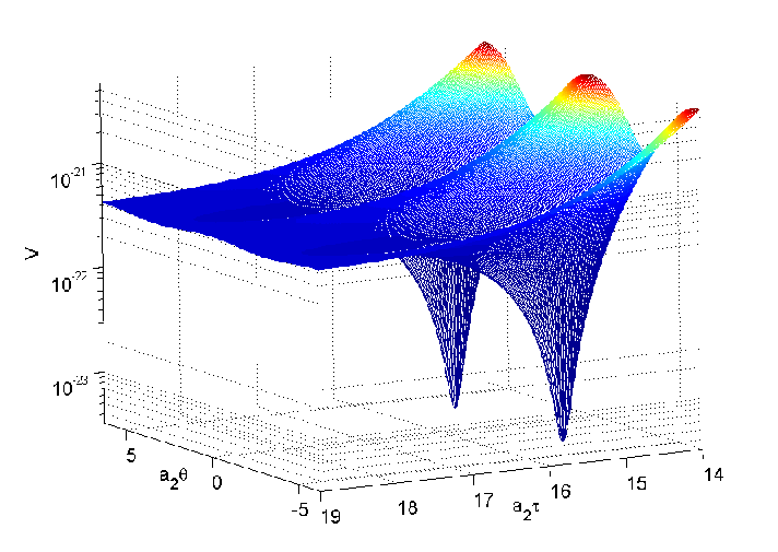
The roulette model is a string theoretic inflationary scenario set in the context of a Type IIB large volume compactification. Although there may be evolution of several Kähler moduli, the observable part of inflation is governed by last (and lightest) one to relax. Since the earlier-evolving moduli stabilize to deep minuma, they rapidly decouple from the dynamics [8], before the final 60 -foldings. The name “roulette” comes from the cyclic shape of the potential, resembling a roulette table whose grooves are the minima toward which the inflaton eventually relaxes (Figure 1). During inflation, the F-term potential of the large volume compactification is flat enough to allow slow-rolling over sizeable patches of field space. Reheating, which we will not address here, occurs when the inflaton fields oscillate at the bottom of the potential. This model was first proposed as a single-field inflation model by Conlon and Quevedo in [3], and subsequently generalized to include the axion as a second inflaton field by Bond, Kofman, Prokushkin and Vaudrevange in ref. [8]. As in ref. [8], we use the large-volume compactification [2], in which the 10 spacetime dimensions of type IIB string theory are separated into a 4-dimensional noncompact spacetime and a conformally Calabi-Yau 3-fold.
After minimizing the F-term potential in the large volume compactification with respect to the axio-dilaton and all Kähler moduli but , the potential can be expressed as a function of and . After expanding in powers of this potential reduces to [8]:
| (1) |
where is the uplifting contribution, of order [3], adjusted so that that at its minimum. It is crucial for the naturalness of Kähler moduli inflation that depends only very weakly upon in the case of interest, where . Because of this, is nearly constant during inflation, and the slow-roll condition on is easily satisfied. Fig. 1 shows the form of the potential.
For notational purposes we define and . The kinetic term takes the diagonal form:
| (2) |
with the component of the Kähler metric given by [8]
| (3) |
In the original Kähler moduli inflation model [3] the Standard Model was confined to a D7-brane that wraps the inflaton cycle. It has recently been pointed out, however, [11] that string loop corrections contribute to the Kähler potential in such a way that the exponential flatness of is destroyed. This would give large contributions to the parameter, thereby preventing slow roll from occuring. Ref. [11] does point out that this can be remedied by removing the D7 brane from the inflating cycle, which has the disadvantage of complicating the reheating process. This could proceed via a mechanism akin to the ones studied in multiple-throat inflationary models in warped compactifications. See for instance ref. [12]. Given that we are only concerned with the inflationary phase in the present Paper, we will take the potential (1) as is.
3 Inflation and nongaussianities
Slow-roll inflationary scenarios generically predict a near-scale invariant spectrum of primordial perturbations, with nearly Gaussian statistics. This is expected, since individual quantum fluctuations can be treated as independent results and should therefore be Gaussian by virtue of the central limit theorem. However, more complex field interactions, along with interactions with gravity, which is inherently non-linear, are sure to produce at least small deviations from Gaussianity. Due to the stochastic nature of these perturbations, it is therefore natural to develop statistical tools to compare predictions of the theory with CMB observations. Wick’s theorem tells us that the even moments (-point correlators) of a linear field or distribution decompose into a sum over the permutations of two-point correlators, whereas the odd moments vanish. The measurement of deviations from gaussianity in a field , can therefore be made through the bispectrum (the Fourier transform of the three-point correlator), and through the connected part of the trispectrum, that is, the part of the Fourier transform of the four-point correlator that cannot be decomposed into products of the power spectrum.
It is common to parameterize the small deviations from gaussianity in terms of their effect on the Bardeen potential through [17]
| (4) |
where is a purely gaussian random field with . Even for large this parameterisation is sufficient, given that the fluctuations are order . Already with the COBE observations it was shown that the nongaussian fraction of must be less than a few percent, (see for example [13]). Subsequent measurements have tightened this limit to the level of . Some recent published limits on are shown in Table 1.
| Komatsu et al. | (WMAP 1-year) | [13] | |
|---|---|---|---|
| Creminelli et al. | (WMAP 3-year) | [14] | |
| Yadav and Wandelt | (WMAP 3-year) | [9] | |
| Komatsu et al. | (WMAP 5-year) | [15] |
Some of these results [9] suggest that the CMB anisotropies exhibit measurable deviations from Gaussian statistics. Whether or not these detections are confirmed, future observations such as the 9-year WMAP data and the Planck satellite data will provide stringent bounds on the primordial bispectrum, yielding additional parameters that any successful model of the early universe will have to match. Although nongaussianities may be measured from the contribution of any connected -point function, the 3-point correlator is the easiest to detect due to the smallness of the anisotropies.
In the original (“local”) ansatz (4), was taken to be a number, but by relating it to the bispectrum one sees that more generally it could be a function of the momenta . Taking the Fourier transform and writing , is easy to show (noting that vanishes identically) that the lowest order nonvanishing component of may be written in terms of the bispectrum and power spectrum:11 1 One must be careful with the sign of , which has been a source of some confusion in the literature, due to the sign difference between the Bardeen potential and the gravitational potential (see appendix A2 of ref. [25].) We use the WMAP convention that positive corresponds to positive bispectrum of .
| (5) |
Due to the delta function, the wave vectors form a triangle, and the -dependence of eq. (5) can be expressed in terms of two ratios of momenta, for example and , and an overall scale. Different mechanisms produce bispectra that peak for differently shaped triangles; for example equilateral (), or squeezed (). The latter corresponds to the prediction of local ansatz. Single-field slow-roll inflation predicts nongaussianity of the local type [18], given that the dominant contribution to the bispectrum should come from the superhorizon influence of small modes which act to “rescale” modes as they evolve toward the end of inflation. A rigorous expansion of the action to third order in perturbation theory is given in ref. [18]. Other models such as ghost inflation and DBI inflation predict large for the equilateral configuration [19], in which non-gaussianities are created before horizon-crossing.
Our focus will be on tracking the perturbative curvature modes from the time they expand beyond the Hubble radius , until the end of inflation. We will use the gradient expansion approach developed by Rigopoulos, Shellard and van Tent [20, 7, 10]. The assumptions of homogeneity and isotropy of the background FRW inflationary universe allow the use of the “long-wavelength” approximation, in which the gradient terms of the equations of motion may be dropped in the classical (unperturbed) equations of motion [20, 16]:
| (6) | |||||
| (7) |
where the Hubble rate is
| (8) |
on scales larger than the Hubble length . As a consequence, the inclusion of metric and field perturbations simply amounts to the inclusion of gradient terms on top of the background, whose equations of motion are computed from the full field equations of motion. The advantage of this approach is twofold: no slow-roll approximation is needed to find and solve the equations of motion, and the resulting equations are exact (non-perturbative) results. Quantitative computation of power spectra and bispectra was done via a perturbative expansion of these gradient equations of motion. The important results of [10] that we made use of are presented in Appendix A. Here we will only sketch the method and refer the reader interested in the details to the Appendix.
For the two-field case such as we consider here, the dynamical degrees of freedom for the metric fluctuations can be reduced to where is the adiabatic curvature fluctuation, is the isocurvature fluctuation, and . ( is like the canonical momentum conjugate to , and the evolution equations are first order in derivatives, similar to Hamilton’s equations of motion. is not an independent degree of freedom, but is constrained in terms of the others.) The formalism solves for the gradient of the three fields, , where . These quantities can furthermore be expanded order-by-order in the cosmological perturbation, . Higher order terms are sourced by the next lowest order ones, through a master equation of the form
| (9) |
where the matrix (see (A.18) is determined by various slow roll parameters. The lowest order source term from which higher order fluctuations follow is deduced by the method of stochastic quantization. This information is encoded in a matrix , eq. (A.20). The solutions of eq. (9) for and which we will need for computing the spectrum and bispectrum can be expressed in terms of a Green’s function which is the solution to
| (10) |
where is the matrix evaluated using just the homogeneous background solution. The main technical difficulty then is in computing the Green’s function. The fluctuation can then be computed through (see eq. (A.31)) and similarly is given by eq. (A.37). The nongaussianity parameter is determined by and through eqs. (A.35) and (A.36) of the appendix.
For the roulette model, we must solve these equations numerically. Analytic results have been developed (e.g., in ref. [7]) in the context of this formalism, but only within certain constrained limits.
4 Numerical method and results
In this section we will consider a number of different parameter sets for the model, indicated in Table 2. Special attention will be given to the first of these, for which we illustrate the different possibilities depending on which inflationary trajectory is followed (i.e., the dependence on the initial conditions). In each case, we evolved the light fields starting from rest, until the end of inflation, which we took to be the point at which the slow roll parameter grew to . For each trajectory, we solved for the perturbation amplitudes to first and second order using the gradient method described above. The power spectrum, scalar spectral index and nonlinearity parameter thus calculated are presented below for a variety of inflationary trajectories and parameter choices. We also discuss the superhorizon influence of the isocurvature modes on these quantities in what follows.
| Set | |||||||
| 1 | 300 | 0.1 | 1 | 0.5 | |||
| 2 | 0.1 | 1 | 0.5 | ||||
| 3 | 0.1 | 1 | 0.5 | ||||
| 4 | 200 | 0.1 | 1 | 0.5 |
In contrast with the KKLT compactifiation, the large volume scenario places no strong restrictions on the value of in the effective field theory [2]. One therefore has considerable freedom to vary the parameters of the potential (1). We first verified the results of ref. [8] as a check on methodology. We solved for the inflation trajectories starting from a variety of initial conditions and verified that slow roll was generically obtained, as found in section 6 of [8]. Some examples are illustrated in Figure 2. Solution A, the “-valley” trajectory of Conlon and Quevedo [3], effectively corresponds to single-field inflation, as the fields start with already minimized. Figure 3 shows a more detailed plot of one of the trajectories, superimposed on a contour plot of the potential. Values of were consistently very small, with at the COBE scale. Typical values of the tensor-to-scalar ratio produced by the fields were therefore .
We focused attention on parameter set 1 of [8], with the modification that the volume was tuned to achieve COBE normalisation (; see Table 2), i.e., the power spectrum is on COBE scales, in order to have a realistic example. This corresponds to an inflationary energy scale GeV, giving a duration of - observable e-foldings of inflation, assuming reheating temperatures of - GeV. Although a more generic method of normalization is to rescale the potential by an overall factor, the dependence on of both terms in the potential gives a way to adjust its magnitude without introducing additional parameters.


| Trajectory | ||||||||
| A | 48.4 | 0 | 0 | 86 | 0.965 | 0.965 | 0 | |
| B | 47.6 | 0.0052 | 0.0069 | 62 | 0.992 | 0.976 | 0.70 | |
| C | 47.0 | 0.0105 | 0.0132 | 72 | 1.02 | 0.940 | 0.81 | |
| D | 46.3 | 0.0242 | 0.0272 | 77 | 1.02 | 0.920 | 0.91 | |
| E | 38.95 | 0.36 | 0.0688 | 0.0698 | 77 | 1.04 | 0.930 | 0.90 |
| F | 38.93 | 0.40 | 0.0068 | 0.0089 | 103 | 1.002 | 0.948 | 0.72 |
| G | 38 | 0.38 | -0.0060 | -0.0060 | 90 | 0.964 | 0.965 | 0.02 |
| Param. set | ||||||||
| 2 | 29.5 | 0.0301 | 0.0338 | 77 | 1.055 | 0.909 | 0.93 | |
| 3 | 28.7 | 0.0553 | 0.0590 | 69 | 1.1045 | 0.849 | 0.97 | |
| 4 | 33.2 | 0.0404 | 0.0442 | 73 | 1.074 | 0.891 | 0.93 | |
| 4 | 35.0 | 0.0060 | 0.0082 | 94 | 1.002 | 0.946 | 0.73 |
4.1 Isocurvature Perturbations
In the case of more highly curved trajectories, the isocurvature modes were found to have a large, positive effect on the power spectrum of adiabatic perturbations, and consequently on the scalar spectral index , as recently shown in [21]. Large curvature in field space during the course of inflation resulted in a “projection” of the isocurvature modes onto the adiabatic direction. For some trajectories with long periods of curving, over 90% of the power spectrum originated from the isocurvature modes. Table 3 gives the proportion of the observable curvature power spectrum at the end of inflation that results from the influence of the isocurvature mode:
| (11) |
where the subscript indicates that these quantities were evaluated at the COBE scale, which we take to be the modes that crossed the horizon 55 e-foldings before the end of inflation. is the power spectrum computed with the effective single-field result
| (12) |
whereas was computed using (A.34). A second result of the influence of isocurvature modes (also discussed in ref. [21]) is a lower scalar spectral index than would be naïvely expected from the single-field result ( in the notation of Appendix A). The full scalar spectral index at COBE scales was computed by taking the derivative of a cubic fit of , with the power spectrum evaluated from (A.34):
| (13) |
Here we have used the fact that in the gauge with approximately constant, . Table 3 gives a comparison of both methods of computing . Our results indicate that a significantly larger power spectrum, along with a generically red-tilted spectrum is an expected result of curved trajectories in roulette inflation. This is of particular interest, given that the most recent cosmological data favor a scalar spectral index of [15].
4.2 Nongaussianities in the roulette model
We now turn to the subject of nongaussianity in the roulette model. Because it gives examples of highly curved field trajectories, one might have hoped to find observably large levels of nongaussianity coming from the isocurvature modes. However, the numerics do not bear out this expectation, as we now describe.
We tested the algorithm for computing from superhorizon evolution of perturbation modes on the two-field quadratic inflation model considered in ref. [10], verified its results. We then analyzed the nonlinear mode evolution for a variety of roulette inflation trajectories, for modes corresponding to a range of horizon exit times before the end of inflation.
The Green’s function in eq. (10) was found by solving the ODE numerically in matrix form, as a function of . This was done once per time step , giving a dimensional array, where corresponds to the number of discrete time steps sampled in the evolution (typically around 1000). Figure 4 shows this behavior for trajectory C of figure 2.

Inflation in the valley, corresponding to the effective one-field scenario of Conlon and Quevedo [3] produced no nongaussianities originating from superhorizon interaction between scalar modes (, where the deviation from zero can be attributed to numerical uncertainty). This is not surprising, since it is the coupling between curvature and isocurvature modes that is expected to generate large bispectra.22 2 Recall that contributions to from the adiabatic fluctuations should give values of order [18]. In more complex inflationary trajectories with sufficient curving in field space, however, we found that values of between and were quite generically produced. But we did not find any examples which produced outside of the small range
| (14) |
This is far below the level of sensitivity foreseen by the PLANCK experiment, for example.
Figure 5 illustrates the time-dependence of at a series of wave-numbers from horizon exit to the end of inflation, for the representative trajectory C in Figure 2), while figure 6 shows the -dependence of after it has stopped evolving. The behaviour of shown is typical for trajectories that continued to curve during most of the period of observable inflation: they produce slightly more pronounced values of during the curved part of the motion, but these values quickly descend to by the end of inflation. The two-field model studied in [10] also exhibits this behaviour: descends to zero as the trajectory straightens out at the end of inflation, resulting in a bispectrum below the level of measurable sensitivity. Table 3 gives some computed values of (where the form an equilateral triangle) at scales that crossed the horizon at e-foldings, as well as for squeezed triangles, with , and corresponding to and respectively. Trajectories labeled A through G are shown in figure 2. The bottom part of table 3 shows results for different parameter sets (given in Table 2). Values of are taken at the end of inflation.

Features in can be understood as being due to curvature of the trajectory at the time of horizon exit of particular modes. Modes that experienced more curving after horizon exit (i.e., those which exited the horizon earlier) produced larger magnitude than those which experienced no curving. These features in the bispectrum are completely absent in single-field inflation. One feature that was common to curved roulette trajectories was a slightly larger bispectrum on large scales, due to the modes which left the horizon before turning in field space occurred. This occurs because only superhorizon-scale modes can experience growth due to the coupling between isocurvature and adiabatic modes (this effect can also be seen in Table 3, which shows the correlation between large isocurvature contributions to the power and larger values of ). Smaller scales which exit the horizon later undergo less such growth. Thus a simultaneous detection of larger in the CMB and smaller primordial non-linearity in large-scale structure may be a way to detect this type of result, if its magnitude can be enhanced to an observable level.
One somewhat nonstandard feature of the roulette model, relative to simpler two-field models, is the nontrivial field metric (eq. (3) which multiplies the kinetic term of the axionic direction . We found that it had no substantial effect on the shape, size, or magnitude of the bispectrum. To test this, we tried replacing by a constant during inflation, and found that the spectrum of observables remained roughly unchanged.
As illustrated in Table 3, the shape-dependence of the observed nongaussianities is as expected from this type of model [19], since nongaussianities from superhorizon evolution are larger in the squeezed configuration, whereas those generated on subhorizon scales (like in DBI inflation) are larger in the equilateral configuration. In all cases, we find that is larger for the squeezed configuration.

5 Discussion
We have studied a model of Kähler moduli inflation built from a realistic construction of Type IIB string theory, using the formalism developed in [20, 7, 10]. We confirm previous results for the power spectrum and the superhorizon influence of isocurvature modes for typical inflationary trajectories. The main new undertaking is a search for nongaussian perturbations from highly curved trajectories. Such deviations from gaussianity can originate from the superhorizon evolution of the second-order curvature perturbation and its interaction with isocurvature perturbations.
When the full spectrum is considered, roulette inflation predicts a smooth power spectrum with a slight red-tilt, in excellent agreement with estimates based on the latest WMAP data. In addition, as shown by [21], the superhorizon influence of isocurvature modes can come to dominate the scalar curvature power spectrum via the relation (A.15). This is the case for inflationary trajectories with large curvature, which can be pictured as a “projection” of the isocurvature perturbation modes onto the adiabatic direction. This contribution, which can account for over 90% of the curvature power spectrum, must therefore be considered in the context of these multiple-field inflationary models.
Concerning the issue of nongaussianity, we did not find examples in which , produced by the mechanism considered in section 4, could be large enough to be observable by future missions; we obtained results which did not exceed the level of expected in conventional single-field inflation models. It was hoped that trajectories with very sharp curving in field space would have yielded larger values, but two considerations could make this difficult. First, if the trajectory relaxes to a straight, effectively single-field form before the end of inflation, damps to zero, as illustrated in figure 1 of ref. [10]. We found trajectories with moderate curving until the end of inflation, which prevented the total erasure of . Multiple-field (“multi-brid”) hybrid inflation models such as discussed in refs. [22, 23] use this effect to produce sizable nongaussianities. Second, large deviation from Gaussianity from this method is correlated with large isocurvature modes being projected onto the curvature direction. If one is able to find models with large , it must be verified that the power-spectrum is not overly amplified and distorted by this effect. This phenomenon is also seen to play an important role in nongaussianity generated by the waterfall fields in hybrid inflation models [24].
However, it is possible that a more complete search of the model’s parameter space would reveal examples with larger values of . In that case, running bispectra (i.e., which depend on the magnitude of the average scale of , as opposed to the shape-dependence), such as we find in the roulette model, could provide an interesting discriminator between models. Recent developments in the detection of nongaussianity via large-scale structure, which would probe at smaller scales, promise to give additional observational handles on such a dependence [25, 26].
It may be interesting to examine other such moduli inflation scenarios that arise once the assumptions of a strict hierarchy of scale are relaxed (for instance, the model of ref. [27] in which the second dynamical field is the inverse overall volume, rather than the axionic partner). A more general study of two-field inflationary models with such an exponentially flat potential would furthermore reveal how generic the above-mentioned behavior is.
Acknowledgments
We thank N. Barnaby, R. Brandenberger, F. Cyr-Racine, S. Prokushkin, G. Rigopoulos and L. Verde for helpful discussions and correspondence. Our research is supported by NSERC (Canada) and FQRNT (Québec).
Appendix A Second order quantities in the gradient expansion formalism
We present here the important results of [10], which were used in the computation of the first- and second-order quantities that formed our main results.
Regardless of the specific inflationary model, we may write the action for a general multifield potential () with minimal gravitational couplings as
| (A.1) |
Here is the Ricci scalar, is the metric in field space and is the reduced Planck mass. We work in units where . At the homogeneous level, and before specifying a choice of spacelike slicing, the FRW metric is , and varying with respect to the fields , and gives the equations of motion for the scalar fields and the Friedmann equations. Here is the time-lapse function, and is the scale factor, from which we define the Hubble parameter . To simplify calculations during inflation, we make the coordinate choice
| (A.2) |
so constant during inflation. Dotted fields will from now on represent differentiation with respect to this time parameter.
Working within the long-wavelength approximation [20], we assume that the fields are homogeneous and isotropic within the horizon. The kinetic term becomes:
| (A.3) |
having defined the velocities
| (A.4) |
We will furthermore define covariant differentiation of a field that transforms as a vector within field space [20]:
| (A.5) | |||||
| (A.6) | |||||
| (A.7) |
where is the connection defined through the metric . Henceforth, uppercase latin indices will represent the various fields, greek will represent spacetime indices, and will be spatial indices. Since we are interested in a two-field inflation model, . In the roulette model there is only one independent connection coefficient:
| (A.8) | |||||
| (A.9) |
For the analysis of the power spectrum and bispectrum, it will furthermore be useful to define the orthonormal basis , where :
| (A.10) |
where and is the antisymmetric tensor. is tangent to the classical field trajectory, whereas is orthogonal. Note that lower and raised indices are equivalent.
The scalar field equations of motion are given in eqs. (8-7). We numerically integrated them to determine the inflationary trajectories. The formalism of [20, 7, 10] which we follow makes extensive use of the “slow roll” parameters,
| (A.11) |
where and are defined in the orthonormal basis (A.10), such that , with the covariant derivatives over the field metric defined above. These quantities are nonlinear, depend on both and , and are not assumed to be small, although they are small in the slow-roll regime. It should be noted that some of them are unintuitively named; for example is proportional to the slope of the potential, in the direction orthogonal to the trajectory, rather than a curvature, and the relation of to the usual slow-roll parameters, with respect to the adiabatic direction, is . Nevertheless we will keep this notation for ease of comparison with ref. [7]. The parameter does agree with the conventional (defined with respect to the slope along the adiabatic direction).
The particular choice of variables we will use to describe the fluctuations in this formalism are
| (A.12) |
which have the property of being invariant under long-wavelength changes of time-slicing [20].This quantity can be projected onto the field basis (A.10):
| (A.13) |
These simplify in the gauge , where . At first order, is the spatial gradient of the usual curvature perturbation, whereas corresponds to the isocurvature perturbation. The gradients are combined, along with their respective velocities , into a 3-component vector,
| (A.14) |
The would-be fourth component is not independent, but is determined to be
| (A.15) |
by the constraint equations [10] which may be derived from the Einstein equations and the definition of , noting that :
| (A.16) | |||||
The relationship between and is nothing more than the well-known “conservation” law of the curvature perturbation. This is valid to all orders, as shown in ref. [28].
Combining these with the equations of motion (6)-(7), the full nonlinear evolution equations may be written in the compact form:
| (A.17) |
The matrix is a function of the parameters defined in eq. (A.11) [10]:
| (A.18) |
Its dominant components are and . The only explicit dependence on the curvature of the field manifold in is the term , but we found that this is negligible () in roulette inflation.
The next step is to solve this system of equations perturbatively. Eq. (A.17) can be expanded into a hierarchy of linear perturbation equations for , each sourced by the previous order. Since we are interested in superhorizon evolution, it is reasonable to take the first-order perturbations to be sourced by a linear perturbation , which encodes the effect of quantum fluctuations at short wavelengths providing the initial values for the long-wavelength modes of interest at horizon crossing. Refs. [7, 20, 10] show that the source term having the right properties is
| (A.19) |
where the creation operator has the standard commutator Superscripts in parentheses indicate the expansion order in perturbation theory.
The matrix of linear solutions around horizon crossing is the slow-roll solution of ref. [10] in which it is argued that deviations from linearity on sub-horizon scales should be slow-roll suppressed:
| (A.20) |
The factor comes from the definition of , and the amplitude is the result we expect from perturbations at horizon crossing.
The window function is designed to source only the superhorizon modes, and the final results must be independent of its exact shape. It is convenient to use a Heaviside step function, , that has support only on scales (recall we are in the gauge ) sufficiently larger than the Hubble radius, where should be of order a few. Given that fluctuations that are generated on sub-horizon scales do not yet feel the effect of curvature, and therefore correspond to fluctuations in Minkowski space, it is reasonable to expect the spectrum of fluctuations on these scales to be Gaussian.
Then
| (A.21) |
where is the time of horizon-crossing of mode
| (A.22) |
Physical quantities are found to be independent of the exact value of .
The first- and second-order equations can then be written:
| (A.23) | |||||
| (A.24) |
Here, (note that is just multiplication by in Fourier space.) is given by [10]:
| (A.25) |
where
| (A.26) |
and
| (A.27) | |||||
| (A.28) | |||||
| (A.29) |
The first index in stands for the row, the second for the column in (A.25), and the third for the “depth” dimension of the array, represented here by a column vector for each . is defined as .
The above linear equations can then be solved with the aid of the Green’s function which is the solution to the inhomogeneous equation
| (A.30) |
with at equal times. This must be solved only once for each classical trajectory, which we do numerically on a grid in , , and . Once is known, the step-function form of simplifies the integration of the first order solution,
| (A.31) | |||||
where we have defined the Fourier-space perturbation as:
| (A.32) |
The second order solution can be expressed, using the same method, as:
| (A.33) |
To connect with observables one transforms the time coordinate in the gauge of uniform expansion time slices () to which describes uniform density slices () [10], so . Then the curvature perturbation can be expressed as the total gradient of a scalar , , which allows observable scalar correlators to be expressed simply. Note that this result should be identical to results found using the formalism, given that the perturbation in the uniform density gauge corresponds exactly to the perturbation in the number of e-folds [29].
The curvature power spectrum is:
| (A.34) |
The scale-dependence of comes as expected from the time-dependence of in (eq. (A.20)), which appears in through eq. (A.31). It should be stressed that the power spectrum here is complete and includes the effect of isocurvature perturbations.
The leading contribution to the bispectrum comes from the expansion to second order in perturbation theory,
| (A.35) | |||||
where [10]
| (A.36) |
The second term in parentheses comes from the coordinate change , and the first term is given by
| (A.37) |
Numerically, we will find that this term dominates over the term in the roulette inflation model by five orders of magnitude. These are all the ingredients needed for evaluation of the nonlinearity parameter [7],
| (A.38) |
References
- [1] S. Kachru, R. Kallosh, A. Linde, and S. P. Trivedi. De Sitter vacua in string theory. Phys. Rev., D68:046005, 2003. [hep-th/0301240]
- [2] J. P. Conlon, F. Quevedo, and K. Suruliz. Large-volume flux compactifications: Moduli spectrum and D3/D7 soft supersymmetry breaking. JHEP, 08:007, 2005. [hep-th/0505076]
- [3] J. P. Conlon and F. Quevedo. Kaehler moduli inflation. JHEP, 01:146, 2006. [hep-th/0509012]
- [4] J. J. Blanco-Pillado et al. Inflating in a better racetrack. JHEP, 09:002, 2006. [hep-th/0603129]
- [5] S. Dimopoulos, S. Kachru, J. McGreevy, and J. G. Wacker. N-flation. JCAP 0808:003,2008 [hep-th/0507205]
- [6] A. Misra, and P. Shukla. Large Volume Axionic Swiss-Cheese Inflation. Nucl. Phys. B800:384-400, 2008. arXiv:0712.1260 [hep-th] A. Misra, and P. Shukla. ’Finite’ Non-Gaussianities and Tensor-Scalar Ratio in Large Volume Swiss-Cheese Compactifications. arXiv:0807.0996 [hep-th]
- [7] G. I. Rigopoulos, E. P. S. Shellard, and B. J. W. van Tent. Large non-Gaussianity in multiple-field inflation. Phys. Rev., D73:083522, 2006. [astro-ph/0506704]
- [8] J. R. Bond, L. Kofman, S. Prokushkin, and P. M. Vaudrevange. Roulette inflation with Kaehler moduli and their axions. Phys. Rev., D75:123511, 2007. [hep-th/0612197]
- [9] A. P. S. Yadav and B. D. Wandelt. Evidence of Primordial Non-Gaussianity (f(NL)) in the Wilkinson Microwave Anisotropy Probe 3-Year Data at 2.8sigma. Phys.Rev.Lett.100:181301,2008 . arXiv:0712.1148 [astro-ph]
- [10] G. I. Rigopoulos, E. P. S. Shellard, and B. J. W. van Tent. Quantitative bispectra from multifield inflation. Phys. Rev., D76:083512, 2007. [astro-ph/0511041]
- [11] M. Cicoli, C. P. Burgess and F. Quevedo. Fibre Inflation: Observable Gravity Waves from IIB String Compactifications, arXiv:0808.0691 [hep-th]
- [12] N. Barnaby, C. P. Burgess and J. M. Cline. Warped reheating in brane-antibrane inflation, JCAP 0504:007, 2005. [hep-th/0412040]
- [13] E. Komatsu et al. First Year Wilkinson Microwave Anisotropy Probe (WMAP) Observations: Tests of Gaussianity. Astrophys. J. Suppl., 148:119–134, 2003. [astro-ph/0302223]
- [14] P. Creminelli, L. Senatore, M. Zaldarriaga, and M. Tegmark. Limits on parameters from WMAP 3yr data. JCAP, 0703:005, 2007. [astro-ph/0610600]
- [15] E. Komatsu et al. Five-Year Wilkinson Microwave Anisotropy Probe (WMAP) Observations:Cosmological Interpretation. 2008. arXiv:0803.0547 [astro-ph]
- [16] D. S. Salopek and J. R. Bond. Nonlinear evolution of long wavelength metric fluctuations in inflationary models. Phys. Rev., D42:3936–3962, 1990.
- [17] E. Komatsu and D. N. Spergel. Acoustic signatures in the primary microwave background bispectrum. Phys. Rev., D63:063002, 2001. [astro-ph/0005036]
- [18] J. M. Maldacena. Non-Gaussian features of primordial fluctuations in single field inflationary models. JHEP, 05:013, 2003. [astro-ph/0210603]
- [19] D. Babich, P. Creminelli, and M. Zaldarriaga. The shape of non-Gaussianities. JCAP, 0408:009, 2004. [astro-ph/0405356]
- [20] G. I. Rigopoulos, E. P. S. Shellard, and B. J. W. van Tent. Non-linear perturbations in multiple-field inflation. Phys. Rev., D73:083521, 2006. [astro-ph/0504508]
- [21] Z. Lalak, D. Langlois, S. Pokorski, and K. Turzynski. Curvature and isocurvature perturbations in two-field inflation. JCAP, 0707:014, 2007. arXiv:0704.0212 [hep-th]
- [22] M. Sasaki. Multi-brid inflation and non-Gaussianity. Prog.Theor.Phys. 120:159-174,2008. arXiv:0805.0974 [astro-ph]
- [23] A. Naruko and M. Sasaki. Large non-Gaussianity from multi-brid inflation. 2008. arXiv:0807.0180 [astro-ph]
- [24] N. Barnaby and J. M. Cline, “Nongaussian and nonscale-invariant perturbations from tachyonic preheating in hybrid inflation,” Phys. Rev. D 73, 106012 (2006) [arXiv:astro-ph/0601481]; “Nongaussianity from tachyonic preheating in hybrid inflation,” Phys. Rev. D 75, 086004 (2007) [arXiv:astro-ph/0611750]. A. Chambers and A. Rajantie, “Lattice calculation of non-Gaussianity from preheating,” Phys. Rev. Lett. 100, 041302 (2008) arXiv:0710.4133 [astro-ph]; “Non-Gaussianity from massless preheating,” JCAP 0808, 002 (2008) arXiv:0805.4795 [astro-ph].
- [25] M. LoVerde, A. Miller, S. Shandera, and L. Verde. Effects of Scale-Dependent Non-Gaussianity on Cosmological Structures. JCAP, 0804:014, 2008. arXiv:0711.4126 [astro-ph]
- [26] F. Lucchin and S. Matarrese, “The Effect of nonGaussian statistics on the mass multiplicity of cosmic structures,” Astrophys. J. 330, 535 (1988). S. Matarrese, L. Verde and R. Jimenez, “The abundance of high-redshift objects as a probe of non-Gaussian initial conditions,” Astrophys. J. 541, 10 (2000) [arXiv:astro-ph/0001366]. L. Verde, R. Jimenez, M. Kamionkowski and S. Matarrese, “Tests for primordial non-Gaussianity,” Mon. Not. Roy. Astron. Soc. 325, 412 (2001) [arXiv:astro-ph/0011180]. R. Scoccimarro, E. Sefusatti and M. Zaldarriaga, “Probing Primordial Non-Gaussianity with Large-Scale Structure,” Phys. Rev. D 69, 103513 (2004) [arXiv:astro-ph/0312286]. E. Sefusatti and E. Komatsu, “The bispectrum of galaxies from high-redshift galaxy surveys: Primordial non-Gaussianity and non-linear galaxy bias,” Phys. Rev. D 76, 083004 (2007) [arXiv:0705.0343 [astro-ph]]. N. Dalal, O. Dore, D. Huterer and A. Shirokov, “The imprints of primordial non-gaussianities on large-scale structure: scale dependent bias and abundance of virialized objects,” Phys. Rev. D 77, 123514 (2008) arXiv:0710.4560 [astro-ph]. A. Slosar, C. Hirata, U. Seljak, S. Ho and N. Padmanabhan, “Constraints on local primordial non-Gaussianity from large scale structure,” arXiv:0805.3580 [astro-ph].
- [27] V. Balasubramanian, P. Berglund, R. Jimenez, J. Simon, and L. Verde. Topology from Cosmology. JHEP 0806:025,2008. arXiv:0712.1815 [hep-th]
- [28] D. H. Lyth, K. A. Malik, and M. Sasaki. A general proof of the conservation of the curvature perturbation. JCAP, 0505:004, 2005. [astro-ph/0411220]
- [29] D. Wands, K. A. Malik, D. H. Lyth, and A. R. Liddle. A new approach to the evolution of cosmological perturbations on large scales. Phys. Rev., D62:043527, 2000. [astro-ph/0003278]