跳到论文正文
W Papers独立论文阅读器 arXiv:0809.2974 论文正文 计算阅读时间 · 0%
引用这篇论文根据当前论文元数据生成,正式投稿前建议核对。


License: arXiv.org perpetual non-exclusive license
arXiv:0809.2974v3 [math.PR] 04 Mar 2010

Thermodynamic Limit for Large Random Trees.

Yuri Bakhtin ††thanks: School of Mathematics, Georgia Tech, Atlanta GA, 30332-0160; email:bakhtin@math.gatech.edu, 404-894-9235 (office phone), 404-894-4409(fax)
Abstract

We consider Gibbs distributions on finite random plane trees with bounded branching. We show that as the order of the tree grows to infinity, the distribution of any finite neighborhood of the root of the tree converges to a limit. We compute the limiting distribution explicitly and study its properties. We introduce an infinite random tree consistent with these limiting distributions and show that it satisfies a certain form of the Markov property. We also study the growth of this tree and prove several limit theorems including a diffusion approximation.

1 Introduction

Various kinds of random trees have been studied in the literature. In this note we consider simply generated random (plane rooted) trees also known as branching processes conditioned on the total population (CBP), see [Ald91b]. Our initial motivation was a study of the secondary structure statistics for large RNA molecules, see [BH08] and [BH09]. The secondary RNA structures can be encoded via plane rooted trees and studied with the help of energy models. In [BH08] and [BH09], it is demonstrated that the naive energy minimization approach to the prediction of typical secondary structure features fails to explain the presence of high degree branchings. However, using the language of statistical mechanics and working with Gibbs ensembles on trees, we were able to include the entropy correction and recover the typical RNA branching type. These results are concerned only with the rough information related to the branching statistics, but in this paper, we suggest a new viewpoint that helps to obtain some insights into the geometry of large random trees.

The model we work with follows the classical Boltzmann–Gibbs postulate stating that the probablity of a configuration TT is proportional to e−β​E​(T)e^{-\beta E(T)}, where E⁡(T)E(T) is the energy of TT, and β\beta is the inverse temperature in appropriate units (see the complete description of our model in Section 2). Gibbs distributions, especially their limiting behaviour under the limit of the size of the system tending to infinity (so called thermodynamic limit), are central to statistical mechanics, see [Sin82] and [Geo88] for a modern mathematical introduction.

The first goal of this paper is to prove that as the order of the tree grows to infinity, the distribution induced by the Gibbs measure converges to that of an infinite discrete tree that we explicitly describe in detail (Sections 2 to 5). This thermodynamic limit belongs to the category of discrete limits of CBP according to the terminology introduced in [Ald91b], and our result (as well as the limiting object) appears to be new. In particular, it does not involve any rerooting procedures like the one introduced in [Ald91a]. We prove the result above for the bounded branching (or out-degree) case, although it should hold true under less restrictive assumptions.

The limiting infinite discrete tree is a more sophisticated object than a classical Galton–Watson tree. In particular, it dies out with zero probability and the progenies of distinct vertices are not independent. However, it turns out that the limiting tree is Markov in a natural sense, and the Markov transition probability is explicitly computed in Section 5. In Section 6 we notice that the number of vertices at a given distance nn from the root also form a Markov chain if nn is understood as a time parameter. We prove that under linear scaling this Markov chain satisfies a limit theorem with the limit given by a gamma distribution. In Section 7 we strengthen this result and show that a functional limit theorem holds with weak convergence to a diffusion process on the positive semi-line with constant drift and diffusion proportional to the square root of the space coordinate. Since this process (under the name of local time for Bessel(3) process) also serves as a scaling limit of the “height profile” for CBP itself, see [Ald91b, Conjecture 7] and [Git98], we can say that the infinite Markov random tree that we construct belongs to the same universality class as the original CBP.

There are several natural and interesting problems arising in connection with our results. One is, obviously, strengthening them to give an alternative to [Git98] proof of the scaling limit in Aldous’s Conjecture 7. Another one is to use our approach to study finer details of the random tree rather than the height profile. Our heuristic computation (see Section 8) shows that the limit can be described as a solution of an SPDE with respect to a Brownian sheet.

Acknowledgements. The author is grateful to NSF for partial support of this research via CAREER award DMS-0742424. He also thanks the referees for their useful comments.

2 The setting and first results on thermodynamic limit

Let us recall that plane trees (or, ordered trees) are rooted trees such that subtrees at any vertex are linearly ordered. In other words, two plane trees and are considered equal if there is a bijection between the vertices of the two trees such that it preserves the parent — child relation on the vertices and preserves the order of the child subtrees of any vertex. Figure 1 shows all plane trees on 44 vertices.

We fix D∈ℕD\in\mathbb{N} and introduce 𝕋N=𝕋N​(D)\mathbb{T}_{N}=\mathbb{T}_{N}(D), the set of all plane trees on NN vertices such that the branching number (i.e. the number of children, or out-degree) of each vertex does not exceed DD. To introduce a Gibbs distribution on 𝕋N\mathbb{T}_{N}, we have to assign an energy value to each tree. We assume that an energy value Ei∈ℝE_{i}\in\mathbb{R} is assigned to every i∈{0,…,D}i\in\{0,\ldots,D\}, and the energy of the tree TT is defined via

E⁡(T)=∑v∈V⁡(T)Edeg⁡(v)=∑i=0Dχi​(T)​Ei,E(T)=\sum_{v\in V(T)}E_{\deg(v)}=\sum_{i=0}^{D}\chi_{i}(T)E_{i},

where V⁡(T)V(T) denotes the set of vertices of the tree TT, deg⁡(v)\deg(v) denotes the branching number of vertex vv, and χi​(T)\chi_{i}(T) is the number of vertices of branching ii in TT. Since the energy of an individual vertex depends only on its immediate neigborhood via the branching number, one can say that this a model with nearest neighbor interaction.

Refer to caption
Figure 1: Five different plane trees of order 4.

Now we fix an inverse temperature parameter β∈ℝ\beta\in\mathbb{R} (usually, in statistical physics β>0\beta>0, but our results apply to other values of β\beta as well) and define a probability measure μN\mu_{N} on 𝕋N\mathbb{T}_{N} by

μN​{T}=e−β​E​(T)ZN,\mu_{N}\{T\}=\frac{e^{-\beta E(T)}}{Z_{N}},

where the normalizing factor (partition function) is defined by

ZN=∑T∈𝕋Ne−β​E​(T).Z_{N}=\sum_{T\in\mathbb{T}_{N}}e^{-\beta E(T)}.

In particular, if β=0\beta=0 or, equivalently, Ei=0E_{i}=0 for all ii, then μN\mu_{N} is a uniform distribution on 𝕋N\mathbb{T}_{N}.

First, we are going to demonstrate that the above model admits a thermodynamic limit, i.e. the sequence of measures (μN)N∈ℕ(\mu_{N})_{N\in\mathbb{N}} has a limit in a certain sense as N→∞N\to\infty. Secondly, we study several curious properties of the limiting infinite random trees.

For each vertex vv of a tree T∈𝕋NT\in\mathbb{T}_{N} its height h⁡(v)h(v) is defined as the distance to the root of TT, i.e. the length of the shortest path connecting vv to the root along the edges of TT. The height of a finite tree is the maximum height of its vertices.

Let n,N∈ℕn,N\in\mathbb{N}. For any plane tree T∈𝕋NT\in\mathbb{T}_{N}, πn,N​T\pi_{n,N}T denotes the neighborhood of the root of radius nn, i.e. the subtree of TT spanned by all vertices with height not exceeding nn.

For any nn and sufficiently large NN, the map πn,N\pi_{n,N} pushes the measure μN\mu_{N} on 𝕋N\mathbb{T}_{N} forward to the measure μN​πn,N−1\mu_{N}\pi_{n,N}^{-1} on SnS_{n}, the set of all trees with height nn.

Theorem 1

For each n∈ℕn\in\mathbb{N}, the measures μN​πn,N−1\mu_{N}\pi_{n,N}^{-1} on SnS_{n} converge in total variation, as N→∞N\to\infty, to a measure PnP_{n}.

A proof of this theorem will be given in Section 3. At this point we prefer to introduce more definitions that will allow us to describe the limiting measures PnP_{n}.

We define

Δ={p=(p0,…,pD)∈[0,1]D+1:∑i=0Dpi=1,∑i=0Dipi=1},\Delta=\left\{p=(p_{0},\ldots,p_{D})\in[0,1]^{D+1}:\ \sum_{i=0}^{D}p_{i}=1,\ \sum_{i=0}^{D}ip_{i}=1\right\},

and let

J⁡(p)=−H⁡(p)+β​E​(p),p∈Δ.J(p)=-H(p)+\beta E(p),\quad p\in\Delta.

where

H(p)=−∑i=0DpilnpiH(p)=-\sum_{i=0}^{D}p_{i}\ln p_{i}

is the entropy of the probability vector p∈Δp\in\Delta, and

E⁡(p)=∑i=0Dpi​EiE(p)=\sum_{i=0}^{D}p_{i}E_{i}

is the associated energy.

The function JJ is used to construct the rate function in the Large Deviation Principle for large plane trees, see [BH08],[BH09].

It is strictly convex and its minimum value on Δ\Delta is attained at a unique point p∗p^{*}. Using Lagrange’s method, we find that

lnpi∗+1+βEi+λ1+iλ2=0,i=0,1,…,D,\ln p_{i}^{*}+1+\beta E_{i}+\lambda_{1}+i\lambda_{2}=0,\quad i=0,1,\ldots,D,

where λ1\lambda_{1} and λ2\lambda_{2} are the Lagrange multipliers. So we see that

p∗i=Ce−β​Eiρi,i=0,1,…,D,p^{*}_{i}=Ce^{-\beta E_{i}}\rho^{i},\quad i=0,1,\ldots,D, (1)

where C=e−1−λ1C=e^{-1-\lambda_{1}}, and ρ=e−λ2\rho=e^{-\lambda_{2}}. In particular,

p∗i>0,i=0,1,…,D.p^{*}_{i}>0,\quad i=0,1,\ldots,D. (2)

Notice that ρ\rho can be characterized as a unique solution of

∑i=0De−β​Ei​ρi=∑i=0Di​e−β​Ei​ρi,\sum_{i=0}^{D}e^{-\beta E_{i}}\rho^{i}=\sum_{i=0}^{D}ie^{-\beta E_{i}}\rho^{i},

and CC may be defined via

1C=∑i=0De−β​Ei​ρi=∑i=0Di​e−β​Ei​ρi.\frac{1}{C}=\sum_{i=0}^{D}e^{-\beta E_{i}}\rho^{i}=\sum_{i=0}^{D}ie^{-\beta E_{i}}\rho^{i}. (3)

We denote J∗=J⁡(p∗)J^{*}=J(p^{*}) and σ=eJ∗\sigma=e^{J^{*}}. For a tree τ∈Sn\tau\in S_{n}, we introduce

E¯​(τ)=∑v∈V⁡(τ)h⁡(v)<nEdeg⁡(v).\bar{E}(\tau)=\sum_{\begin{subarray}{c}v\in V(\tau)\\ h(v)<n\end{subarray}}E_{\deg(v)}. (4)

Notice that the summation above excludes the highest level of the tree.

Theorem 2

For any n∈ℕn\in\mathbb{N}, the limiting probability measure PnP_{n} is given by

Pn​{τ}=Qn​k​ρk​σm​e−β​E¯​(τ)P_{n}\{\tau\}=Q_{n}k\rho^{k}\sigma^{m}e^{-\beta\bar{E}(\tau)} (5)

where the tree τ∈Sn\tau\in S_{n} is assumed to have kk vertices of height nn and mm vertices of height less than nn. The constant QnQ_{n} is a normalizing factor.

We give a proof of Theorems 1 and 2 in the next Section 3. In Section 4 we compute the value of QnQ_{n} explicitly. In Section 5 we shall see that our convergence results may be interpreted as convergence to an infinite random tree.

Remark 1

Although Theorems 1 and 2 do not hold in full generality for D=∞D=\infty, we expect that there is a large class of energy functions for which analogous results are true.

3 Proof of Theorems 1 and 2

For both theorems it is sufficient to check that for any nn and any two trees τ1,τ2∈Sn\tau_{1},\tau_{2}\in S_{n},

limN→∞μN​πn,N−1​{τ1}μN​πn,N−1​{τ2}=k1​e−β​E¯​(τ1)​ρk1​σm1k2​e−β​E¯​(τ2)​ρk2​σm2,\lim_{N\to\infty}\frac{\mu_{N}\pi_{n,N}^{-1}\{\tau_{1}\}}{\mu_{N}\pi_{n,N}^{-1}\{\tau_{2}\}}=\frac{k_{1}e^{-\beta\bar{E}(\tau_{1})}\rho^{k_{1}}\sigma^{m_{1}}}{k_{2}e^{-\beta\bar{E}(\tau_{2})}\rho^{k_{2}}\sigma^{m_{2}}}, (6)

where we assume that τ1\tau_{1} has k1k_{1} vertices of height nn, and m1m_{1} vertices of height less than nn; τ2\tau_{2} has k2k_{2} vertices of height nn, and m2m_{2} vertices of height less than nn.

The energy of each tree TT with πn,N​T=τ1\pi_{n,N}T=\tau_{1} is composed of contributions from the vertices of the tree τ1\tau_{1} of height less than nn (we call this contribution E¯​(τ1)\bar{E}(\tau_{1}), see (4)) and the contribution from the plane forest on N−m1N-m_{1} vertices with k1k_{1} connected components. The same applies to τ2\tau_{2}.

Let us recall (see e.g. Theorem 5.3.10 in [Sta99]) that the number of plane forests on NN vertices with kk components and r0,r1,…,rDr_{0},r_{1},\ldots,r_{D} vertices with branching numbers, respectively, 0,1,…,D0,1,\ldots,D is

kN​(Nr0,r1,…,rD)\frac{k}{N}\binom{N}{r_{0},\ r_{1},\ \ldots,\ r_{D}}

if r0+…+rD=Nr_{0}+\ldots+r_{D}=N, r1+2​r2+…+D​rD=N−kr_{1}+2r_{2}+\ldots+Dr_{D}=N-k, and 00 otherwise.

Therefore,

μN​πn,N−1​{τ1}μN​πn,N−1​{τ2}\displaystyle\frac{\mu_{N}\pi_{n,N}^{-1}\{\tau_{1}\}}{\mu_{N}\pi_{n,N}^{-1}\{\tau_{2}\}} =e−β​E¯​(τ1)​∑r∈Δ⁡(N,m1,k1)k1N−m1​(N−m1r0,r1,…,rD)​e−β​E​(r)e−β​E¯​(τ2)​∑r∈Δ⁡(N,m2,k2CLOSEk2N−m2​(N−m2r0,r1,…,rD)​e−β​E​(r)\displaystyle=\frac{e^{-\beta\bar{E}(\tau_{1})}\sum_{r\in\Delta(N,m_{1},k_{1})}\frac{k_{1}}{N-m_{1}}\binom{N-m_{1}}{r_{0},\ r_{1},\ \ldots,\ r_{D}}e^{-\beta E(r)}}{e^{-\beta\bar{E}(\tau_{2})}\sum_{r\in\Delta(N,m_{2},k_{2}}\frac{k_{2}}{N-m_{2}}\binom{N-m_{2}}{r_{0},\ r_{1},\ \ldots,\ r_{D}}e^{-\beta E(r)}}
=e−β​E¯​(τ1)​I1​(N)e−β​E¯​(τ2)​I2​(N).\displaystyle=\frac{e^{-\beta\bar{E}(\tau_{1})}I_{1}(N)}{e^{-\beta\bar{E}(\tau_{2})}I_{2}(N)}. (7)

Here

Δ(N,m,k)={r∈ℤ+D+1:r0+…+rD=N−m,r1+2r2+…+DrD=N−m−k},\Delta(N,m,k)=\{r\in\mathbb{Z}_{+}^{D+1}:\ r_{0}+\ldots+r_{D}=N-m,\\ r_{1}+2r_{2}+\ldots+Dr_{D}=N-m-k\},

and ℤ+=ℕ∪{0}\mathbb{Z}_{+}=\mathbb{N}\cup\{0\}.

Fix any ε>0\varepsilon>0 and define

Δ⁡(N,m,k,ε)={r∈Δ⁡(N,m,k):|rN−m−p∗|<ε}.\Delta(N,m,k,\varepsilon)=\left\{r\in\Delta(N,m,k):\ \left|\frac{r}{N-m}-p^{*}\right|<\varepsilon\right\}.

We claim that

I1​(N)=I1​(N,ε)​(1+o⁡(1)),N→∞,I_{1}(N)=I_{1}(N,\varepsilon)(1+o(1)),\quad N\to\infty, (8)

where

I1​(N,ε)=∑r∈Δ⁡(N,m1,k1,ε)k1N−m1​(N−m1r0,r1,…,rD)​e−β​E​(r).I_{1}(N,\varepsilon)=\sum_{r\in\Delta(N,m_{1},k_{1},\varepsilon)}\frac{k_{1}}{N-m_{1}}\binom{N-m_{1}}{r_{0},\ r_{1},\ \ldots,\ r_{D}}e^{-\beta E(r)}.

In fact, using Stirling’s formula we see that if ri≠0r_{i}\neq 0 for all i=0,…,Di=0,\ldots,D,

k1N−m1​(N−m1r0,r1,…,rD)​e−β​E​(r)\displaystyle\frac{k_{1}}{N-m_{1}}\binom{N-m_{1}}{r_{0},\ r_{1},\ \ldots,\ r_{D}}e^{-\beta E(r)}
=k1​(N−m1)N−m1−12​e−β​E​(r)​eθN−m112​(N−m1)−θr012​r0−…−θrD12​rD(2​π)D2​r0r0+12​…​rDrD+12\displaystyle=\frac{k_{1}(N-m_{1})^{N-m_{1}-\frac{1}{2}}e^{-\beta E(r)}e^{\frac{\theta_{N-m_{1}}}{12(N-m_{1})}-\frac{\theta_{r_{0}}}{12r_{0}}-\ldots-\frac{\theta_{r_{D}}}{12r_{D}}}}{(2\pi)^{\frac{D}{2}}r_{0}^{r_{0}+\frac{1}{2}}\ldots r_{D}^{r_{D}+\frac{1}{2}}}
=k1​e−(N−m1)​J​(rN−m1)((N−m1)​r0​…​rD)12⋅eθN−m112​(N−m1)−θr012​r0−…−θrD12​rD(2​π)D2,\displaystyle=\frac{k_{1}e^{-(N-m_{1})J(\frac{r}{N-m_{1}})}}{((N-m_{1})r_{0}\ldots r_{D})^{\frac{1}{2}}}\cdot\frac{e^{\frac{\theta_{N-m_{1}}}{12(N-m_{1})}-\frac{\theta_{r_{0}}}{12r_{0}}-\ldots-\frac{\theta_{r_{D}}}{12r_{D}}}}{(2\pi)^{\frac{D}{2}}},

with 0<θj<10<\theta_{j}<1 for all j∈ℕj\in\mathbb{N}. If NN is sufficiently large, there is a vector r∗​(N)∈Δ⁡(N,m1,k1,ε)r^{*}(N)\in\Delta(N,m_{1},k_{1},\varepsilon) such that |r∗​(N)N−m1−p∗|<ε/2|\frac{r^{*}(N)}{N-m_{1}}-p^{*}|<\varepsilon/2. Due to the strong convexity of JJ, there is a number δ>0\delta>0 independent of NN such that

minΔ⁡(N,m1,k1)∖Δ⁡(N,m1,k1,ε)⁡J⁡(rN−m1)>J⁡(r∗​(N)N−m1)+δ,\min_{\Delta(N,m_{1},k_{1})\setminus\Delta(N,m_{1},k_{1},\varepsilon)}J\left(\frac{r}{N-m_{1}}\right)>J\left(\frac{r^{*}(N)}{N-m_{1}}\right)+\delta,

so that the contribution from each element of  Δ⁡(N,m1,k1)∖Δ⁡(N,m1,k1,ε)\Delta(N,m_{1},k_{1})\setminus\Delta(N,m_{1},k_{1},\varepsilon) is exponentially smaller than that of r∗​(N)r^{*}(N) as N→∞N\to\infty. The statement follows since the number of elements in Δ⁡(N,m1,k1)∖Δ⁡(N,m1,k1,ε)\Delta(N,m_{1},k_{1})\setminus\Delta(N,m_{1},k_{1},\varepsilon) is bounded by ND+1N^{D+1}. This argument can be easily extended to the case where ri=0r_{i}=0 for some ii, which completes the proof of our claim (8).

Let us now define for r∈Δ⁡(N,m1,k1,ε)r\in\Delta(N,m_{1},k_{1},\varepsilon),

b⁡(r)=(r0+(k2−k1),r1−(k2−k1)−(m2−m1),r2,r3,…,rD).b(r)=(r_{0}+(k_{2}-k_{1}),r_{1}-(k_{2}-k_{1})-(m_{2}-m_{1}),r_{2},r_{3},\ldots,r_{D}).

Notice that for sufficiently small ε\varepsilon and sufficiently large NN, the image Δ′​(N,ε)\Delta^{\prime}(N,\varepsilon) of Δ⁡(N,m1,k1,ε)\Delta(N,m_{1},k_{1},\varepsilon) under bb is a subset of Δ⁡(N,m2,k2)\Delta(N,m_{2},k_{2}). Moreover, bb is invertible and, therefore, establishes a bijection between Δ⁡(N,m1,k1,ε)\Delta(N,m_{1},k_{1},\varepsilon) and Δ′​(N,ε)\Delta^{\prime}(N,\varepsilon).

Introducing

I2​(N,ε)=∑r∈Δ′​(N,ε)k2N−m2​(N−m2r0,r1,…,rD)​e−β​E​(r),I_{2}(N,\varepsilon)=\sum_{r\in\Delta^{\prime}(N,\varepsilon)}\frac{k_{2}}{N-m_{2}}\binom{N-m_{2}}{r_{0},\ r_{1},\ \ldots,\ r_{D}}e^{-\beta E(r)},

and using exactly the same reasoning as for I1I_{1}, we see that

I2​(N)=I2​(N,ε)​(1+o⁡(1)),N→∞.I_{2}(N)=I_{2}(N,\varepsilon)(1+o(1)),\quad N\to\infty. (9)

Equations (7),(8),(9) imply now that

μN​πn,N−1​{τ1}μN​πn,N−1​{τ2}\displaystyle\frac{\mu_{N}\pi_{n,N}^{-1}\{\tau_{1}\}}{\mu_{N}\pi_{n,N}^{-1}\{\tau_{2}\}} =e−β​E¯​(τ1)​I1​(N,ε)e−β​E¯​(τ2)​I2​(N,ε)​(1+o⁡(1))\displaystyle=\frac{e^{-\beta\bar{E}(\tau_{1})}I_{1}(N,\varepsilon)}{e^{-\beta\bar{E}(\tau_{2})}I_{2}(N,\varepsilon)}(1+o(1))
=k1​e−β​E¯​(τ1)k2​e−β​E¯​(τ2)⋅∑r∈Δ⁡(N,m1,k1,ε)a1,r∑r∈Δ⁡(N,m1,k1,ε)a2,r​(1+o⁡(1)),N→∞,\displaystyle=\frac{k_{1}e^{-\beta\bar{E}(\tau_{1})}}{k_{2}e^{-\beta\bar{E}(\tau_{2})}}\cdot\frac{\sum_{r\in\Delta(N,m_{1},k_{1},\varepsilon)}a_{1,r}}{\sum_{r\in\Delta(N,m_{1},k_{1},\varepsilon)}a_{2,r}}(1+o(1)),\quad N\to\infty, (10)

where

a1,r=(N−m1r0,r1,…,rD)​e−β​E​(r),a_{1,r}=\binom{N-m_{1}}{r_{0},\ r_{1},\ \ldots,\ r_{D}}e^{-\beta E(r)},

and

a2,r=(N−m2r0+(k2−k1),r1−(k2−k1+m2−m1),r2,…,rD)​e−β​E​(b⁡(r)).a_{2,r}=\binom{N-m_{2}}{r_{0}+(k_{2}-k_{1}),r_{1}-(k_{2}-k_{1}+m_{2}-m_{1}),r_{2},\ldots,r_{D}}e^{-\beta E(b(r))}.

Assuming that k1≥k2k_{1}\geq k_{2} and m1≥m2m_{1}\geq m_{2} (all the other cases can be treated in the same way), we get

a1,ra2,r=((r1−(k2−k1)−(m2−m1))​…​(r1+1)CLOSEOPEN(N−m2)​…​(N−m1+1))⋅(r0​…​(r0+(k2−k1)+1))​R,\frac{a_{1,r}}{a_{2,r}}=\frac{((r_{1}-(k_{2}-k_{1})-(m_{2}-m_{1}))\ldots(r_{1}+1)}{(N-m_{2})\ldots(N-m_{1}+1))\cdot(r_{0}\ldots(r_{0}+(k_{2}-k_{1})+1))}R,

where

R=R⁡(k1,m1,k2,m2)=eβ⁡(E0−E1)​(k2−k1)−β​E1​(m2−m1).R=R(k_{1},m_{1},k_{2},m_{2})=e^{\beta(E_{0}-E_{1})(k_{2}-k_{1})-\beta E_{1}(m_{2}-m_{1})}.

Due to the definition of Δ⁡(N,m,k,ε)\Delta(N,m,k,\varepsilon),

a1,ra2,r≤((p1∗+ε)​(N−m1)−(k2−k1)−(m2−m1))−(k2−k1)−(m2−m1)(N−m1)−(m2−m1)​((p0∗−ε)​(N−m1)+(k2−k1))−(k2−k1)​R,\frac{a_{1,r}}{a_{2,r}}\leq\frac{((p_{1}^{*}+\varepsilon)(N-m_{1})-(k_{2}-k_{1})-(m_{2}-m_{1}))^{-(k_{2}-k_{1})-(m_{2}-m_{1})}}{(N-m_{1})^{-(m_{2}-m_{1})}((p_{0}^{*}-\varepsilon)(N-m_{1})+(k_{2}-k_{1}))^{-(k_{2}-k_{1})}}R,

so that

lim supN→∞supr∈Δ⁡(N,m,k,ε)a1,ra2,r\displaystyle\limsup_{N\to\infty}\sup_{r\in\Delta(N,m,k,\varepsilon)}\frac{a_{1,r}}{a_{2,r}} ≤(p1∗+ε)−(m2−m1)​(p1∗+εp0∗−ε)−(k2−k1)​R\displaystyle\leq(p_{1}^{*}+\varepsilon)^{-(m_{2}-m_{1})}\left(\frac{p_{1}^{*}+\varepsilon}{p_{0}^{*}-\varepsilon}\right)^{-(k_{2}-k_{1})}R
≤(e−β​E1p1∗+ε)m2−m1​((p0∗−ε)​eβ⁡(E0−E1)p1∗+ε)k2−k1\displaystyle\leq\left(\frac{e^{-\beta E_{1}}}{p_{1}^{*}+\varepsilon}\right)^{m_{2}-m_{1}}\left(\frac{(p_{0}^{*}-\varepsilon)e^{\beta(E_{0}-E_{1})}}{p_{1}^{*}+\varepsilon}\right)^{k_{2}-k_{1}} (11)

In the same way,

lim infN→∞infr∈Δ⁡(N,m,k,ε)a1,ra2,r≥(e−β​E1p1∗−ε)m2−m1​((p0∗+ε)​eβ⁡(E0−E1)p1∗−ε)k2−k1\liminf_{N\to\infty}\inf_{r\in\Delta(N,m,k,\varepsilon)}\frac{a_{1,r}}{a_{2,r}}\geq\left(\frac{e^{-\beta E_{1}}}{p_{1}^{*}-\varepsilon}\right)^{m_{2}-m_{1}}\left(\frac{(p_{0}^{*}+\varepsilon)e^{\beta(E_{0}-E_{1})}}{p_{1}^{*}-\varepsilon}\right)^{k_{2}-k_{1}} (12)

Since the choice of ε\varepsilon is arbitrary, relations (10),(11), and (12) imply that

limN→∞μN​πn,N−1​{τ1}μN​πn,N−1​{τ2}=k1​e−β​E¯​(τ1)k2​e−β​E¯​(τ2)​(e−β​E1p1∗)m2−m1​(p0∗​eβ⁡(E0−E1)p1∗)k2−k1.\lim_{N\to\infty}\frac{\mu_{N}\pi_{n,N}^{-1}\{\tau_{1}\}}{\mu_{N}\pi_{n,N}^{-1}\{\tau_{2}\}}=\frac{k_{1}e^{-\beta\bar{E}(\tau_{1})}}{k_{2}e^{-\beta\bar{E}(\tau_{2})}}\left(\frac{e^{-\beta E_{1}}}{p_{1}^{*}}\right)^{m_{2}-m_{1}}\left(\frac{p_{0}^{*}e^{\beta(E_{0}-E_{1})}}{p_{1}^{*}}\right)^{k_{2}-k_{1}}. (13)

Using (1), we see that

p0∗​eβ⁡(E0−E1)p1∗=1ρ.\frac{p_{0}^{*}e^{\beta(E_{0}-E_{1})}}{p_{1}^{*}}=\frac{1}{\rho}. (14)

A direct computation based on (1) and (3) implies

H⁡(p∗)=−ln⁡(C​ρ)+β​E​(p∗).H(p^{*})=-\ln(C\rho)+\beta E(p^{*}).

Therefore,

e−β​E1p1∗=1C​ρ=e−J⁡(p∗)=1σ.\frac{e^{-\beta E_{1}}}{p_{1}^{*}}=\frac{1}{C\rho}=e^{-J(p^{*})}=\frac{1}{\sigma}. (15)

Now, (6) is an immediate consequence of (13),(14), and (15).     □\Box

4 Consistency and the precise value of QnQ_{n}

We begin with the following consistency property:

Theorem 3

The family of measures (Pn)n∈ℕ(P_{n})_{n\in\mathbb{N}} is consistent, i.e. for any nn and any τ∈Sn\tau\in S_{n}

Pn​{τ}=∑τ′∈Sn+1πnn+1​τ′=τPn+1​{τ′},P_{n}\{\tau\}=\sum_{\begin{subarray}{c}\tau^{\prime}\in S_{n+1}\\ \pi_{n}^{n+1}\tau^{\prime}=\tau\end{subarray}}P_{n+1}\{\tau^{\prime}\},

where πnn+1\pi_{n}^{n+1} denotes the projection map from Sn+1S_{n+1} to SnS_{n}.

Proof: This theorem is a direct consequence of the limiting procedure in Theorem 1. However, it is interesting to derive it from the specific form of PnP_{n} provided by Theorem 2.

Let us assume that τ∈Sn\tau\in S_{n}, and τ\tau has nn vertices of height kk and mm of height less than nn.

∑τ′∈Sn+1πnn+1​τ=τPn+1​{τ′}\displaystyle\sum_{\begin{subarray}{c}\tau^{\prime}\in S_{n+1}\\ \pi_{n}^{n+1}\tau=\tau\end{subarray}}P_{n+1}\{\tau^{\prime}\}
=Qn+1​∑i1,…,ik=0De−β⁡(E¯​(τ)+Ei1+…+Eik)​(i1+…+ik)​ρi1+…+ik​σm+k\displaystyle=Q_{n+1}\sum_{i_{1},\ldots,i_{k}=0}^{D}e^{-\beta(\bar{E}(\tau)+E_{i_{1}}+\ldots+E_{i_{k}})}(i_{1}+\ldots+i_{k})\rho^{i_{1}+\ldots+i_{k}}\sigma^{m+k}
=Qn+1​e−β​E¯​(τ)​σm+k​∑i1,…,ik=0De−β⁡(E1+…+Ek)​(i1+…+ik)​ρi1+…+ik\displaystyle=Q_{n+1}e^{-\beta\bar{E}(\tau)}\sigma^{m+k}\sum_{i_{1},\ldots,i_{k}=0}^{D}e^{-\beta(E_{1}+\ldots+E_{k})}(i_{1}+\ldots+i_{k})\rho^{i_{1}+\ldots+i_{k}}
=Qn+1​e−β​E¯​(τ)​σm+k​k​∑i1=0D(i1​ρi1​e−β​Ei)​∑i2=0D(ρi2​e−β​Ei2)​…​∑ik=0D(ρik​e−β​Eik)\displaystyle=Q_{n+1}e^{-\beta\bar{E}(\tau)}\sigma^{m+k}k\sum_{i_{1}=0}^{D}(i_{1}\rho^{i_{1}}e^{-\beta E_{i}})\sum_{i_{2}=0}^{D}(\rho^{i_{2}}e^{-\beta E_{i_{2}}})\ldots\sum_{i_{k}=0}^{D}(\rho^{i_{k}}e^{-\beta E_{i_{k}}})
=Qn+1​e−β​E¯​(τ)​σm+k​k​1C​(1C)k−1.\displaystyle=Q_{n+1}e^{-\beta\bar{E}(\tau)}\sigma^{m+k}k\frac{1}{C}\left(\frac{1}{C}\right)^{k-1}.

In this calculation we denoted by i1,…,iki_{1},\ldots,i_{k} the branching numbers of the vertices of height nn. We used the definition of PnP_{n} in the first identity. The second identity is just a convenient rearrangement. The third one follows from the symmetry in the factor (i1+…+ik)(i_{1}+\ldots+i_{k}). In the last identity we used (3) and the fact that p∗∈Δp^{*}\in\Delta. Identity  (15) implies

1C=ρσ,\frac{1}{C}=\frac{\rho}{\sigma}, (16)

so that

∑τ′∈Sn+1πnn+1​τ=τPn+1​{τ′}=Qn+1​e−β​E¯​(τ)​σm+k​k​σ−k​ρk=Qn+1Qn​Pn​{τ}.\sum_{\begin{subarray}{c}\tau^{\prime}\in S_{n+1}\\ \pi_{n}^{n+1}\tau=\tau\end{subarray}}P_{n+1}\{\tau^{\prime}\}=Q_{n+1}e^{-\beta\bar{E}(\tau)}\sigma^{m+k}k\sigma^{-k}\rho^{k}=\frac{Q_{n+1}}{Q_{n}}P_{n}\{\tau\}. (17)

Since this holds true for all τ∈Sn\tau\in S_{n}, we can conclude that Qn=Qn+1Q_{n}=Q_{n+1} which completes the proof.    □\Box

Identity (17) means that the constant Q=QnQ=Q_{n} in Theorem 2 is the same for all nn. Choosing n=1n=1 we can compute it using (5):

1=Q​∑k=1Dk​e−β​Ek​ρk​σ1=Q​σC.1=Q\sum_{k=1}^{D}ke^{-\beta E_{k}}\rho^{k}\sigma^{1}=\frac{Q\sigma}{C}.

A more precise version of Theorem 2 easily follows:

Theorem 4

Let CC be defined by (3). For each nn, the limiting probability measure PnP_{n} is given by

Pn​{τ}=C​k​e−β​E¯​(τ)​ρk​σm−1,P_{n}\{\tau\}=Cke^{-\beta\bar{E}(\tau)}\rho^{k}\sigma^{m-1},

where the tree τ∈Sn\tau\in S_{n} is assumed to have kk vertices of height nn and mm vertices of height less than nn.

5 The limiting random tree

Let S∞S_{\infty} be the set of infinite plane trees with branching number bounded by DD. Theorem 3 along with the classical Daniell—Kolmogorov Consistency theorem (see [Bil99]) allows us to introduce a measure P∞P_{\infty} on S∞S_{\infty} consistent with measures PnP_{n} for all nn. Intuitively this is clear, but to make it precise we need to introduce a coding of plane trees. We have chosen one of several possible coding schemes.

Let TT be a plane tree (finite or infinite) with branching bounded by DD. Then TT has a finite number rn≤Dnr_{n}\leq D^{n} of vertices of any given height nn. Let us say that all vertices of the same height nn form the nn-th level of the tree. The vertices of nn-th level are naturally ordered and can be enumerated by numbers from 11 to rnr_{n} (except for the case when there are no vertices at nn-th level at all). Each of rnr_{n} vertices of the nn-th level has a parent at the level n−1n-1. Denote the number received by the parent of ll-th vertex of the nn-th level under the described enumeration by gn,lg_{n,l}. If rn<l≤Dnr_{n}<l\leq D^{n} we set gn,l=0g_{n,l}=0. We also agree that for the root of the tree, i.e., the first vertex in the zeroth level, g0,1=1g_{0,1}=1.

Then for any n≥0n\geq 0 the nn-th level can be encoded by a vector

gn=(gn,1,…,gn,Dn)∈{0,1,…,Dn−1}Dn,g_{n}=(g_{n,1},\ldots,g_{n,D^{n}})\in\{0,1,\ldots,D^{n-1}\}^{D^{n}},

and the whole tree can be identified with the sequence of levels

(g1,g2,…)∈𝕏=∏n=1∞{0,1,…,Dn−1}Dn,(g_{1},g_{2},\ldots)\in\mathbb{X}=\prod_{n=1}^{\infty}\{0,1,\ldots,D^{n-1}\}^{D^{n}},

so that the space 𝕋\mathbb{T} of all plane trees (finite or infinite) with branching bounded by DD can be identified with a subset of 𝕏\mathbb{X}.

Theorem 5

There is a unique measure P∞P_{\infty} on 𝕋\mathbb{T} such that it is consistent with measures PnP_{n}:

P∞​πn−1=Pn,P_{\infty}\pi_{n}^{-1}=P_{n},

where πn\pi_{n} denotes the root’s neighbourhood of height nn of a tree from 𝕋\mathbb{T}. This measure is concentrated on S∞S_{\infty}.

Proof: The first statement follows from Theorem 3 and the Consistency theorem. The second statement is a consequence of the fact that for each n∈ℕn\in\mathbb{N}, PnP_{n} is concentrated on trees with positive number of vertices at nn-th level.     □\Box

The space 𝕏\mathbb{X} is compact in the product topology. Therefore, the convergence of finite-dimensional distributions established in Theorem 1 and the classical Prokhorov theorem (see e.g. [Bil99]) imply the following result:

Theorem 6

As N→∞N\to\infty, measures PNP_{N} viewed as measures on 𝕏\mathbb{X} converge weakly to P∞P_{\infty} in the product topology.

This statement shows that there is a limiting object for the random trees that we consider. This object is an infinite random tree. For any n∈ℕn\in\mathbb{N}, the first nn levels of this random tree are distributed according to PnP_{n}.

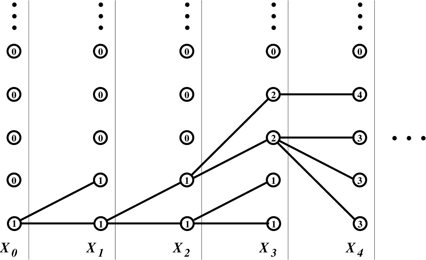
Let us now embed the space 𝕏\mathbb{X} into 𝕏¯=(ℤ+ℕ)ℤ+\bar{\mathbb{X}}=(\mathbb{Z}_{+}^{\mathbb{N}})^{\mathbb{Z}_{+}} filling up all the unused coordinates with zeros. The measure P∞P_{\infty} can be treated as a measure on 𝕏¯\bar{\mathbb{X}} thus generating a ℤ+ℕ\mathbb{Z}_{+}^{\mathbb{N}}-valued process (Xn)n=0∞(X_{n})_{n=0}^{\infty} with discrete time. This process along with the associated random tree is visualized on Figure 2. For any nn, the map XnX_{n} describes how the nn-th level of the tree is built upon the n−1n-1-th one.

Refer to caption
Figure 2: A realization of the process (Xn)(X_{n}) and the associated random tree

For a level g:ℕ→ℤ+g:\mathbb{N}\to\mathbb{Z}_{+}, we denote by |g||g| the number of non-zero entries in gg (i.e. the number of vertices at the level). For two levels gg and g′g^{\prime} we write g⊲g′g\lhd g^{\prime} if maxl⁡gl′≤|g|\max_{l}g^{\prime}_{l}\leq|g|. If g⊲g′g\lhd g^{\prime} then we define

E(g,g′)=∑i=1|g|E#⁡{j:gj′=i},E(g,g^{\prime})=\sum_{i=1}^{|g|}E_{\#\{j:\ g^{\prime}_{j}=i\}},

the energy induced by level g′g^{\prime} at its parent level gg.

Theorem 4 immediately implies the following result:

Theorem 7

The process (Xn)(X_{n}) defined above is Markov with transition probability

𝖯⁡{Xn+1=g′|Xn=g}={|g′||g|​e−β​E​(g,g′)​ρ|g′|−|g|​σ|g|,g⊲g′,0,otherwise.\mathsf{P}\{X_{n+1}=g^{\prime}|\ X_{n}=g\}=\begin{cases}\frac{|g^{\prime}|}{|g|}e^{-\beta E(g,g^{\prime})}\rho^{|g^{\prime}|-|g|}\sigma^{|g|},&g\lhd g^{\prime},\\ 0,&\mbox{\rm otherwise.}\end{cases}

6 A limit theorem for the size of nn-th level

Let us introduce Yn=|Xn|Y_{n}=|X_{n}|, the random number of vertices at nn-th level. The following statement is a direct consequence of Theorem 4 or Theorem 7:

Theorem 8

The process (Yn)n=0∞(Y_{n})_{n=0}^{\infty} is Markov with transition probability

𝖯⁡{Yn+1=k′|Yn=k}=k′k​ρk′−k​σk​∑0≤i1,…,ik≤Di1+…+ik=k′e−β⁡(Ei1+…+Eik).\mathsf{P}\{Y_{n+1}=k^{\prime}|\ Y_{n}=k\}=\frac{k^{\prime}}{k}\rho^{k^{\prime}-k}\sigma^{k}\sum_{\begin{subarray}{c}0\leq i_{1},\ldots,i_{k}\leq D\\ i_{1}+\ldots+i_{k}=k^{\prime}\end{subarray}}e^{-\beta(E_{i_{1}}+\ldots+E_{i_{k}})}.

The next theorem shows that in fact YnY_{n} grows linearly in time. Let

μ=B2−1,\mu=B_{2}-1, (18)

where

Bn=∑i=0Din​pi∗,n∈ℕ.B_{n}=\sum_{i=0}^{D}i^{n}p^{*}_{i},\quad n\in\mathbb{N}.

Then μ>0\mu>0 being the variance of p∗p^{*}, a nondegenerate distribution.

Theorem 9
Ynn⋅2μ→L​a​wΓ,\frac{Y_{n}}{n}\cdot\frac{2}{\mu}\stackrel{{\scriptstyle Law}}{{\to}}\Gamma,

where Γ\Gamma is a random variable with density

p⁡(t)={t​e−t,t≥00,t<0p(t)=\begin{cases}te^{-t},&t\geq 0\\ 0,&t<0\end{cases}

Proof: Let us find the Laplace transform (generating function) of the distribution of YnY_{n}:

Ln​(s)=𝖤​es​Yn,s≤0,L_{n}(s)=\mathsf{E}e^{sY_{n}},\quad s\leq 0,

(this definition differs from the traditional one by a sign change of the argument) and prove that for any x≤0x\leq 0,

limn→∞Ln​(xn)=1(1−μ​x2)2=:L∞​(x),\lim_{n\to\infty}L_{n}\left(\frac{x}{n}\right)=\frac{1}{\left(1-\frac{\mu x}{2}\right)^{2}}=:L_{\infty}(x), (19)

the r.h.s. being the Laplace transform of

p⁡(t)=4​tμ2​e−2​tμ,p(t)=\frac{4t}{\mu^{2}}e^{-\frac{2t}{\mu}},

the density of the r.v. μ2​Γ\frac{\mu}{2}\Gamma.This will imply the desired result, see e.g. [Kal86, Appendix 5] for various statements on Laplace transforms.

Theorem 8 and (16) imply

𝖤⁡[es​Yn+1|Yn=k]=∑k′es​k′​k′k​ρk′−k​σk​∑0≤i1,…,ik≤Di1+…+ik=k′e−β⁡(Ei1+…+Eik)\displaystyle\mathsf{E}\left[e^{sY_{n+1}}|Y_{n}=k\right]=\sum_{k^{\prime}}\frac{e^{sk^{\prime}}k^{\prime}}{k}\rho^{k^{\prime}-k}\sigma^{k}\sum_{\begin{subarray}{c}0\leq i_{1},\ldots,i_{k}\leq D\\ i_{1}+\ldots+i_{k}=k^{\prime}\end{subarray}}e^{-\beta(E_{i_{1}}+\ldots+E_{i_{k}})}
=σkk​ρk​∑0≤i1,…,ik≤D(i1+…+ik)​ρi1+…+ik​es⁡(i1+…+ik)​e−β⁡(Ei1+…+Eik)\displaystyle=\frac{\sigma^{k}}{k\rho^{k}}\sum_{0\leq i_{1},\ldots,i_{k}\leq D}(i_{1}+\ldots+i_{k})\rho^{i_{1}+\ldots+i_{k}}e^{s(i_{1}+\ldots+i_{k})}e^{-\beta(E_{i_{1}}+\ldots+E_{i_{k}})}
=w⁡(s)​v​(s)k−1,\displaystyle=w(s)v(s)^{k-1},

where

v⁡(s)=∑i=0Dpi∗​es​i=∑i=0DC​ρi​e−β​Ei​es​i,v(s)=\sum_{i=0}^{D}p^{*}_{i}e^{si}=\sum_{i=0}^{D}C\rho^{i}e^{-\beta E_{i}}e^{si},

and

w⁡(s)=∑i=0Di​pi∗​es​i=∑i=0DC​i​ρi​e−β​Ei​es​i=v′​(s).w(s)=\sum_{i=0}^{D}ip^{*}_{i}e^{si}=\sum_{i=0}^{D}Ci\rho^{i}e^{-\beta E_{i}}e^{si}=v^{\prime}(s).

Therefore,

Ln+1​(s)=𝖤​w​(s)​v​(s)Yn−1=w⁡(s)v⁡(s)​𝖤​eln⁡v⁡(s)​Yn=z⁡(s)​Ln​(f⁡(s)),L_{n+1}(s)=\mathsf{E}w(s)v(s)^{Y_{n}-1}=\frac{w(s)}{v(s)}\mathsf{E}e^{\ln v(s)Y_{n}}=z(s)L_{n}(f(s)), (20)

where

f⁡(s)=ln⁡v⁡(s),f(s)=\ln v(s), (21)

and

z⁡(s)=w⁡(s)v⁡(s)=f′​(s).z(s)=\frac{w(s)}{v(s)}=f^{\prime}(s).

Both zz and ff are analytic functions. An elementary calculation shows that

f⁡(s)=s+μ2​s2+r⁡(s),f(s)=s+\frac{\mu}{2}s^{2}+r(s),

and

ln⁡z⁡(s)=μ​s+q⁡(s),\ln z(s)=\mu s+q(s),

where μ=w′​(0)−1\mu=w^{\prime}(0)-1 was introduced in (18) and

|r⁡(s)|≤c​|s|3,|q⁡(s)|≤c​|s|2|r(s)|\leq c|s|^{3},\quad|q(s)|\leq c|s|^{2} (22)

for some c>0c>0 and all s≤0s\leq 0.

From now on, x≤0x\leq 0 is fixed. Using (20) and the obvious identity

L0​(s)=es,L_{0}(s)=e^{s},

we can write

Ln​(xn)=z⁡(xn)⋅z⁡(f⁡(xn))⋅z⁡(f2​(xn))⋅…⋅z⁡(fn−1​(xn))​efn​(xn),L_{n}\left(\frac{x}{n}\right)=z\left(\frac{x}{n}\right)\cdot z\left(f\left(\frac{x}{n}\right)\right)\cdot z\left(f^{2}\left(\frac{x}{n}\right)\right)\cdot\ldots\cdot z\left(f^{n-1}\left(\frac{x}{n}\right)\right)e^{f^{n}\left(\frac{x}{n}\right)},

where

fk​(x)=f∘f​…∘f⏟k​(x),k≥0,f^{k}(x)=\underbrace{f\circ f\ldots\circ f}_{k}(x),\quad k\geq 0,

so that we have to study the numbers (xn,k)n∈ℕ,k=0,…,n(x_{n,k})_{n\in\mathbb{N},k=0,\ldots,n} defined by

xn,k=fk​(xn).x_{n,k}={f}^{k}\left(\frac{x}{n}\right).

We shall compare (xn,k)n∈ℕ,k=0,…,n(x_{n,k})_{n\in\mathbb{N},k=0,\ldots,n} to (yn,k)n∈ℕ,k=0,…,n(y_{n,k})_{n\in\mathbb{N},k=0,\ldots,n} defined by

yn,k=1nx−μ2​k.y_{n,k}=\frac{1}{\frac{n}{x}-\frac{\mu}{2}k}.

For fixed nn, both sequences (xn,k)(x_{n,k}) and (yn,k)(y_{n,k}) are negative and increasing in kk. Therefore

|xn,k|≤|xn,0|=|x|n,|x_{n,k}|\leq|x_{n,0}|=\frac{|x|}{n},

and

|yn,k|≤|yn,0|=|x|n.|y_{n,k}|\leq|y_{n,0}|=\frac{|x|}{n}.

Let us prove that for sufficiently large nn and any kk between 00 and nn,

|yn,k−xn,k|≤k⁡(μ24+c)​(|x|n)3.|y_{n,k}-x_{n,k}|\leq k\left(\frac{\mu^{2}}{4}+c\right)\left(\frac{|x|}{n}\right)^{3}. (23)

This is certainly true for k=0k=0. For the induction step, we write

|yn,k−xn,k|≤|yn,k−f⁡(yn,k−1)|+|f⁡(yn,k−1)−f⁡(xn,k−1)|=I1+I2.|y_{n,k}-x_{n,k}|\leq|y_{n,k}-f(y_{n,k-1})|+|f(y_{n,k-1})-f(x_{n,k-1})|=I_{1}+I_{2}.

A straightforward computation based on (21) shows that

|I1|=|μ24​yn,k−12​yn,k+r⁡(yn,k−1)|≤(μ24+c)​(|x|n)3|I_{1}|=\left|\frac{\mu^{2}}{4}y_{n,k-1}^{2}y_{n,k}+r(y_{n,k-1})\right|\leq\left(\frac{\mu^{2}}{4}+c\right)\left(\frac{|x|}{n}\right)^{3}

Since |f′​(s)|≤1|f^{\prime}(s)|\leq 1 for all sufficiently small ss, we see that

|I2|≤|yn,k−1−xn,k−1|.|I_{2}|\leq|y_{n,k-1}-x_{n,k-1}|.

Combining these estimates we see that

|yn,k−xn,k|≤(μ24+c)​(|x|n)3+|yn,k−1−xn,k−1|,|y_{n,k}-x_{n,k}|\leq\left(\frac{\mu^{2}}{4}+c\right)\left(\frac{|x|}{n}\right)^{3}+|y_{n,k-1}-x_{n,k-1}|,

and our claim (23) follows. It immediately implies that

|yn,k−xn,k|≤Cn2|y_{n,k}-x_{n,k}|\leq\frac{C}{n^{2}} (24)

for some K=K⁡(x)K=K(x), sufficiently large nn and all kk. We can now write

ln⁡Ln​(xn)\displaystyle\ln L_{n}\left(\frac{x}{n}\right) =∑k=0n−1ln⁡z⁡(xn,k)+xn,n\displaystyle=\sum_{k=0}^{n-1}\ln z(x_{n,k})+x_{n,n}
=∑k=0n−1μ​xn,k+∑k=0n−1q⁡(xn,k)+xn,n\displaystyle=\sum_{k=0}^{n-1}\mu x_{n,k}+\sum_{k=0}^{n-1}q(x_{n,k})+x_{n,n}
=∑k=0n−1μ​yn,k+∑k=0n−1μ⁡(xn,k−yn,k)+∑k=0n−1q⁡(xn,k)+xn,n\displaystyle=\sum_{k=0}^{n-1}\mu y_{n,k}+\sum_{k=0}^{n-1}\mu(x_{n,k}-y_{n,k})+\sum_{k=0}^{n-1}q(x_{n,k})+x_{n,n}
=I1+I2+I3+I4.\displaystyle=I_{1}+I_{2}+I_{3}+I_{4}.

It is straightforward to see that limn→∞I2+I3+I4=0\lim_{n\to\infty}I_{2}+I_{3}+I_{4}=0. The first term

I1=μ​∑k=0n−11nx−μ2​k=μ​x​1n​∑k=0n−111−μ​x2​kn\displaystyle I_{1}=\mu\sum_{k=0}^{n-1}\frac{1}{\frac{n}{x}-\frac{\mu}{2}k}=\mu x\frac{1}{n}\sum_{k=0}^{n-1}\frac{1}{1-\frac{\mu x}{2}\frac{k}{n}}

can be viewed as a Riemann integral sum, so that

limn→∞ln⁡Ln​(xn)=μ​x​∫01d​u1−μ​x2​u=−2​ln⁡(1−μ​x2),\lim_{n\to\infty}\ln L_{n}\left(\frac{x}{n}\right)=\mu x\int_{0}^{1}\frac{du}{1-\frac{\mu x}{2}u}=-2\ln\left(1-\frac{\mu x}{2}\right),

which immediately implies (19).     □\Box

7 A functional limit theorem

In this section we prove the following theorem on diffusion approximation for the process YY:

Theorem 10

Let

Zn​(t)=Y[n​t]n,n∈ℕ,t∈ℝ+.Z_{n}(t)=\frac{Y_{[nt]}}{n},\quad n\in\mathbb{N},t\in\mathbb{R}_{+}.

Then, as n→∞n\to\infty, the distribution of ZnZ_{n} converges weakly in the Skorokhod topology in D[0,∞)D[0,\infty) to the unique nonnegative weak solution ZZ of the stochastic Itô equation

d​Z​(t)\displaystyle dZ(t) =μ​d​t+μ​Z​(t)​d​W​(t),\displaystyle=\mu dt+\sqrt{\mu Z(t)}dW(t),
Z⁡(0)\displaystyle Z(0) =0.\displaystyle=0.

Proof: Since the initial point Z⁡(0)=0Z(0)=0 is an “entrance and non-exit” singular point for the positive semi-axis (see the classification of singular points in [IM74] ), the existence and uniqueness of a nonnegative solution for all positive times is guaranteed. Let us define

b⁡(x)≡μ,and​a​(x)=μ⋅max⁡{x,0},x∈ℝ,b(x)\equiv\mu,\quad\text{and}\ a(x)=\mu\cdot\max\{x,0\},\quad x\in\mathbb{R},

and extend the equation above to the negative semi-axis by

d​Z​(t)=b⁡(Z⁡(t))​d​t+a⁡(Z⁡(t))​d​W​(t).dZ(t)=b(Z(t))dt+\sqrt{a(Z(t))}dW(t). (25)

An obvious argument shows that there is no solution starting at 00 and being negative for some t>0t>0. Therefore the weak existence and uniqueness in law hold for (25). According to Section 5.4B of [KS98], this existence and uniqueness is equivalent to the well-posedness of the martingale problem associated with bb and aa.

We will use Theorem 4.1 from [EK86, Chapter 7] on diffusion approximation. The coefficients a,ba,b were defined on the whole real line so as the theorem applies directly, with no modification. We proceed to check its conditions.

We must find processes AnA_{n} and BnB_{n} with the following properties:

  1. 1.

    Trajectories of AnA_{n} and BnB_{n} are in D[0,∞)D[0,\infty).

  2. 2.

    AnA_{n} is nondecreasing.

  3. 3.

    Mn=Zn−BnM_{n}=Z_{n}-B_{n} and Mn2−AnM_{n}^{2}-A_{n} are martingales with respect to the natural filtration generated by Zn,An,BnZ_{n},A_{n},B_{n}.

  4. 4.

    For every T>0T>0 the following holds true:

    limn→∞𝖤​supt≤T|Zn​(t)−Zn​(t−)|2\displaystyle\lim_{n\to\infty}\mathsf{E}\sup_{t\leq T}|Z_{n}(t)-Z_{n}(t-)|^{2} =0,\displaystyle=0, (26)
    limn→∞𝖤​supt≤T|An​(t)−An​(t−)|\displaystyle\lim_{n\to\infty}\mathsf{E}\sup_{t\leq T}|A_{n}(t)-A_{n}(t-)| =0,\displaystyle=0, (27)
    limn→∞𝖤​supt≤T|Bn​(t)−Bn​(t−)|2\displaystyle\lim_{n\to\infty}\mathsf{E}\sup_{t\leq T}|B_{n}(t)-B_{n}(t-)|^{2} =0,\displaystyle=0, (28)
    supt≤T|Bn​(t)−∫0tb⁡(Zn​(s))​𝑑s|=supt≤T|Bn​(t)−μ​t|\displaystyle\sup_{t\leq T}\left|B_{n}(t)-\int_{0}^{t}b(Z_{n}(s))ds\right|=\sup_{t\leq T}\left|B_{n}(t)-\mu t\right| →𝖯0,n→∞,\displaystyle\stackrel{{\scriptstyle\mathsf{P}}}{{\to}}0,\quad n\to\infty, (29)
    supt≤T|An​(t)−∫0ta⁡(Zn​(s))​𝑑s|\displaystyle\sup_{t\leq T}\left|A_{n}(t)-\int_{0}^{t}a(Z_{n}(s))ds\right| →𝖯0,n→∞.\displaystyle\stackrel{{\scriptstyle\mathsf{P}}}{{\to}}0,\quad n\to\infty. (30)

We shall need the following lemma:

Lemma 1
𝖤⁡[Yj+1|Yj=k]=\displaystyle\mathsf{E}[Y_{j+1}|Y_{j}=k]= μ+k,\displaystyle\mu+k,
𝖤⁡[Yj+12|Yj=k]=\displaystyle\mathsf{E}[Y_{j+1}^{2}|Y_{j}=k]= B3+3​(k−1)​B2+(k−1)​(k−2),\displaystyle B_{3}+3(k-1)B_{2}+(k-1)(k-2),
𝖤⁡[Yj+13|Yj=k]=\displaystyle\mathsf{E}[Y_{j+1}^{3}|Y_{j}=k]= B4+4​(k−1)​B3+6​(k−1)​(k−2)​B2+3​(k−1)​B22\displaystyle B_{4}+4(k-1)B_{3}+6(k-1)(k-2)B_{2}+3(k-1)B_{2}^{2}
+(k−1)​(k−2)​(k−3),\displaystyle+(k-1)(k-2)(k-3),
𝖤⁡[Yj+14|Yj=k]=\displaystyle\mathsf{E}[Y_{j+1}^{4}|Y_{j}=k]= B5+5​(k−1)​B4+10​(k−1)​(k−2)​B3+10​(k−1)​B3​B2\displaystyle B_{5}+5(k-1)B_{4}+10(k-1)(k-2)B_{3}+10(k-1)B_{3}B_{2}
+15​(k−1)​(k−2)​B22+10​(k−1)​(k−2)​(k−3)​B2\displaystyle+15(k-1)(k-2)B_{2}^{2}+10(k-1)(k-2)(k-3)B_{2}
+(k−1)​(k−2)​(k−3)​(k−4).\displaystyle+(k-1)(k-2)(k-3)(k-4).

Proof: For the first of these identities, we write

𝖤⁡[Yj+1|Yj=k]\displaystyle\mathsf{E}[Y_{j+1}|\ Y_{j}=k] =σkk​ρk​∑0≤i1,…,ik≤D(i1+…+ik)2​ρi1+…+ik​e−β⁡(Ei1+…+Eik)\displaystyle=\frac{\sigma^{k}}{k\rho^{k}}\sum_{0\leq i_{1},\ldots,i_{k}\leq D}(i_{1}+\ldots+i_{k})^{2}\rho^{i_{1}+\ldots+i_{k}}e^{-\beta(E_{i_{1}}+\ldots+E_{i_{k}})}
=1k[k(∑i1=0Di12Cρi1e−β​Ei1)(∑i2=0DCρi2e−β​Ei2)k−1\displaystyle=\frac{1}{k}\Biggl[k\left(\sum_{i_{1}=0}^{D}i_{1}^{2}C\rho^{i_{1}}e^{-\beta E_{i_{1}}}\right)\left(\sum_{i_{2}=0}^{D}C\rho^{i_{2}}e^{-\beta E_{i_{2}}}\right)^{k-1}
+k(k−1)(∑i1=0Di1Cρi1e−β​Ei1)2(∑i2=0DCρi2e−β​Ei2)k−2]\displaystyle+k(k-1)\left(\sum_{i_{1}=0}^{D}i_{1}C\rho^{i_{1}}e^{-\beta E_{i_{1}}}\right)^{2}\left(\sum_{i_{2}=0}^{D}C\rho^{i_{2}}e^{-\beta E_{i_{2}}}\right)^{k-2}\Biggr]
=1k​(k​B2+k⁡(k−1))=B2+k−1\displaystyle=\frac{1}{k}(kB_{2}+k(k-1))=B_{2}+k-1
=μ+k,\displaystyle=\mu+k,

where we used the symmetry of the terms (i12+…​ik2)(i_{1}^{2}+\ldots i_{k}^{2}), i1​i2+i1​i3+…+ik−1​iki_{1}i_{2}+i_{1}i_{3}+\ldots+i_{k-1}i_{k} and (16). Next,

𝖤⁡[Yj+12|Yj=k]\displaystyle\mathsf{E}[Y_{j+1}^{2}|\ Y_{j}=k] =σkk​ρk​∑0≤i1,…,ik≤D(i1+…+ik)3​ρi1+…+ik​e−β⁡(Ei1+…+Eik)\displaystyle=\frac{\sigma^{k}}{k\rho^{k}}\sum_{0\leq i_{1},\ldots,i_{k}\leq D}(i_{1}+\ldots+i_{k})^{3}\rho^{i_{1}+\ldots+i_{k}}e^{-\beta(E_{i_{1}}+\ldots+E_{i_{k}})}
=1k​(k​B3+3​k​(k−1)​B2+k⁡(k−1)​(k−2))\displaystyle=\frac{1}{k}\bigl(kB_{3}+3k(k-1)B_{2}+k(k-1)(k-2)\bigr)
=B3+3​(k−1)​B2+(k−1)​(k−2),\displaystyle=B_{3}+3(k-1)B_{2}+(k-1)(k-2),

and the other two identities in the statement of the lemma can be obtained in a similar way.     □\Box

Returning to the proof of the functional limit theorem, let us find the coefficient Bn​(t)B_{n}(t) first. The process ZnZ_{n} is constant on any interval of the form [j/n,(j+1)/n)[j/n,(j+1)/n). Due to Lemma 1,

𝖤[Zn(t+1n)|Zn(t)]=Zn(t)+μ1n,\mathsf{E}\left.\left[Z_{n}\left(t+\frac{1}{n}\right)\right|Z_{n}(t)\right]=Z_{n}(t)+\mu\frac{1}{n}, (31)

so that we can set Bn​(t)=μ⁡[n​t]/nB_{n}(t)=\mu[nt]/n to satisfy the martingale requirement on Mn=Zn−BnM_{n}=Z_{n}-B_{n}. Notice that with this choice of BnB_{n}, relations (28) and (29) are easily seen to be satisfied. Lemma 1 also implies

𝖤[Z2n(t+1n)|Zn(t)]=B3+3​(n​Zn​(t)−1)​B2+(n​Zn​(t)−1)​(n​Zn​(t)−2)n2,\mathsf{E}\left.\left[Z^{2}_{n}\left(t+\frac{1}{n}\right)\right|Z_{n}(t)\right]\\ =\frac{B_{3}+3(nZ_{n}(t)-1)B_{2}+(nZ_{n}(t)-1)(nZ_{n}(t)-2)}{n^{2}}, (32)

so that for t∈1n​ℤt\in\frac{1}{n}\mathbb{Z},

𝖤[Mn2(t+1n)−Mn2(t)|Zn(t)]=1nμZn(t)+1n2(B3−B22−B2+1).\mathsf{E}\left.\left[M^{2}_{n}\left(t+\frac{1}{n}\right)-M^{2}_{n}(t)\right|Z_{n}(t)\right]=\frac{1}{n}\mu Z_{n}(t)+\frac{1}{n^{2}}(B_{3}-B_{2}^{2}-B_{2}+1).

Therefore we can set

An(t)=∑j:jn≤t(μnZn(jn)+[n​t]n2(B3−B22−B2+1)),A_{n}(t)=\sum_{j:\frac{j}{n}\leq t}\left(\frac{\mu}{n}Z_{n}\left(\frac{j}{n}\right)+\frac{[nt]}{n^{2}}(B_{3}-B_{2}^{2}-B_{2}+1)\right),

to satisfy the martingale requirement on Mn2−AM_{n}^{2}-A. Notice that AnA_{n} is nondecreasing since

1n​μ​Zn​(t)+1n2​(B3−B22−B2+1)\displaystyle\frac{1}{n}\mu Z_{n}(t)+\frac{1}{n^{2}}(B_{3}-B_{2}^{2}-B_{2}+1) ≥1n2​(B2−1)+1n2​(B3−B22−B2+1)\displaystyle\geq\frac{1}{n^{2}}(B_{2}-1)+\frac{1}{n^{2}}(B_{3}-B_{2}^{2}-B_{2}+1)
≥1n2​(B3−B22)≥0,\displaystyle\geq\frac{1}{n^{2}}(B_{3}-B_{2}^{2})\geq 0,

where the last inequality follows from the Cauchy—Schwartz inequality and B1=1B_{1}=1. So properties 1–3 are satisfied, and (30) follows from the definitions of aa and AA, and the convergence

limn→∞supt≤T∑j:jn≤t1n2(B2−1)+1n2(B3−B22−B2+1)=0.\lim_{n\to\infty}\sup_{t\leq T}\sum_{j:\frac{j}{n}\leq t}\frac{1}{n^{2}}(B_{2}-1)+\frac{1}{n^{2}}(B_{3}-B_{2}^{2}-B_{2}+1)=0.

To prove (27) we use the definition of AA to write

𝖤​supt≤T|An​(t)−An​(t−)|≤μn​𝖤​supjn≤TZn​(jn)+1n2​(B3−B22−B2+1)\mathsf{E}\sup_{t\leq T}|A_{n}(t)-A_{n}(t-)|\leq\frac{\mu}{n}\mathsf{E}\sup_{\frac{j}{n}\leq T}Z_{n}\left(\frac{j}{n}\right)+\frac{1}{n^{2}}(B_{3}-B_{2}^{2}-B_{2}+1)

so it suffices to prove that 𝖤​supjn≤TZn​(jn)\mathsf{E}\sup_{\frac{j}{n}\leq T}Z_{n}\left(\frac{j}{n}\right) is bounded. The definition of MnM_{n}, Lyapunov’s inequality and Doob’s maximal inequality for submartingales imply that for some c>0c>0:

𝖤​supjn≤TZn​(jn)\displaystyle\mathsf{E}\sup_{\frac{j}{n}\leq T}Z_{n}\left(\frac{j}{n}\right) ≤μ​T+𝖤​supjn≤T|Mn​(jn)|\displaystyle\leq\mu T+\mathsf{E}\sup_{\frac{j}{n}\leq T}\left|M_{n}\left(\frac{j}{n}\right)\right|
≤μ​T+c​𝖤​Mn2​(T)\displaystyle\leq\mu T+c\sqrt{\mathsf{E}M^{2}_{n}(T)}
≤μ​T+c​2​(𝖤​Zn2​(T)+μ2​T2).\displaystyle\leq\mu T+c\sqrt{2(\mathsf{E}Z^{2}_{n}(T)+\mu^{2}T^{2})}.

Lemma 1 implies that 𝖤​Zn2​(T)\mathsf{E}Z^{2}_{n}(T) has a limit, as n→∞n\to\infty, so that (27) is verified.

A lengthy but elementary calculation based on Lemma 1 shows that

𝖤⁡[(Yj+1−Yj)4|Yn]≤c⁡(Yj2+1)\mathsf{E}[(Y_{j+1}-Y_{j})^{4}|Y_{n}]\leq c(Y_{j}^{2}+1)

for some constant c>0c>0, so that we can write

𝖤​supt≤T(Zn​(t)−Zn​(t−))2\displaystyle\mathsf{E}\sup_{t\leq T}(Z_{n}(t)-Z_{n}(t-))^{2} ≤[𝖤​supt≤T(Zn​(t)−Zn​(t−))4]1/2\displaystyle\leq\left[\mathsf{E}\sup_{t\leq T}(Z_{n}(t)-Z_{n}(t-))^{4}\right]^{1/2}
≤[1n4∑j:jn≤T𝖤(Yj+1−Yj)4]1/2\displaystyle\leq\left[\frac{1}{n^{4}}\sum_{j:\frac{j}{n}\leq T}\mathsf{E}(Y_{j+1}-Y_{j})^{4}\right]^{1/2}
≤[cn4​∑j≤n​T𝖤⁡(Yj2+1)]1/2\displaystyle\leq\left[\frac{c}{n^{4}}\sum_{j\leq nT}\mathsf{E}(Y_{j}^{2}+1)\right]^{1/2}

Since Lemma 1 implies that for some constant c1>0c_{1}>0,

𝖤⁡(Yj2+1)≤c1​j2,j∈ℕ,\mathsf{E}(Y_{j}^{2}+1)\leq c_{1}j^{2},\quad j\in\mathbb{N},

we conclude that

𝖤​supt≤T(Zn​(t)−Zn​(t−))2\displaystyle\mathsf{E}\sup_{t\leq T}(Z_{n}(t)-Z_{n}(t-))^{2} ≤cn4⋅n⋅c1​n2​T2→0,n→∞,\displaystyle\leq\sqrt{\frac{c}{n^{4}}\cdot n\cdot c_{1}n^{2}T^{2}}\to 0,\quad n\to\infty,

and the proof of the theorem is complete.     □\Box

8 Diffusion limit for finer structure of the random tree

In this section we present a non-rigorous and sketchy description for the diffusion limit of the infinite Markov random tree itself rather then its width given by YnY_{n} at time nn. Let us fix any time n0n_{0} and divide all Yn0Y_{n_{0}} vertices into rr nonempty disjoint groups. For any n≥n0n\geq n_{0} denote the progeny of ii-th group at time nn by Vi,nV_{i,n}.

We want to study the coevolution of (V1,n,…,Vr,n)(V_{1,n},\ldots,V_{r,n}). Though each Vi,nV_{i,n} is not a Markov process, it is elementary to see that the whole vector is a homogeneous Markov process. We would like to compute the diffusion limit for this vector under an appropriate rescaling:

1n​(V1,[n​t],…,Vr,[n​t])\frac{1}{n}(V_{1,[nt]},\ldots,V_{r,[nt]})

We need to find the local drift and diffusion coefficients for the limiting process. Let j1+…+jr=kj_{1}+\ldots+j_{r}=k. Then computations similiar to Lemma 1 produce

𝖤⁡[V1,m+1n−j1n|1n​(V1,[n​t],…,Vr,[n​t])=1n​(j1,…,jr)]=μ​j1/nk/n​1n,\mathsf{E}\left[\frac{V_{1,m+1}}{n}-\frac{j_{1}}{n}\Bigr|\ \frac{1}{n}(V_{1,[nt]},\ldots,V_{r,[nt]})=\frac{1}{n}(j_{1},\ldots,j_{r})\right]=\mu\frac{j_{1}/n}{k/n}\frac{1}{n},

so, by symmetry, the local limit drift is

bi​(v)=μ​viv1+…+vr.b_{i}(v)=\mu\frac{v_{i}}{v_{1}+\ldots+v_{r}}.

Similarly, the diagonal terms for local diffusion:

𝖤\displaystyle\mathsf{E} [(V1,m+1n−j1n)2|1n​(V1,[n​t],…,Vr,[n​t])=1n​(j1,…,jr)]\displaystyle\left[\left(\frac{V_{1,m+1}}{n}-\frac{j_{1}}{n}\right)^{2}\Bigr|\ \frac{1}{n}(V_{1,[nt]},\ldots,V_{r,[nt]})=\frac{1}{n}(j_{1},\ldots,j_{r})\right]
=μ​j1n​1+B3−3​B2+2kn,\displaystyle=\mu\frac{j_{1}}{n}\frac{1+\frac{B_{3}-3B_{2}+2}{k}}{n},

and

ai​i​(v)=μ​vi.a_{ii}(v)=\mu v_{i}.

For the off-diagonal terms a computation produces

𝖤[(V1,m+1−j1)(V2,m+1−j2)|V1,m=j1,…,Vr,m=jm]=0,\displaystyle\mathsf{E}[(V_{1,m+1}-j_{1})(V_{2,m+1}-j_{2})|\ V_{1,m}=j_{1},\ldots,V_{r,m}=j_{m}]=0,

so that

ai​j≡0,i≠j.a_{ij}\equiv 0,\quad i\neq j.

So, the limiting equations are

dVi(t)=μVi​(t)∑jVj​(t)dt+μ​Vi​(t)𝟏{Vi>0}dWi(t).dV_{i}(t)=\mu\frac{V_{i}(t)}{\sum_{j}V_{j}(t)}dt+\sqrt{\mu V_{i}(t)}{\bf 1}_{\{V_{i}>0\}}dW_{i}(t).

Let us introduce cumulative counts

Uj=V1+…+Vj.U_{j}=V_{1}+\ldots+V_{j}.

Then Z​(t)=Ur​(t)Z(t)=U_{r}(t), and

dUj=μUjUrdt+μ​U1𝟏{U1>0}dW1+……+μ⁡(Uj−Uj−1)𝟏{Uj−Uj−1>0}dWjdU_{j}=\mu\frac{U_{j}}{U_{r}}dt+\sqrt{\mu U_{1}}{\bf 1}_{\{U_{1}>0\}}dW_{1}+\ldots\\ \ldots+\sqrt{\mu(U_{j}-U_{j-1})}{\bf 1}_{\{U_{j}-U_{j-1}>0\}}dW_{j} (33)

Then, for each 0≤u1≤…≤ur0\leq u_{1}\leq\ldots\leq u_{r}, we can solve this equation with initial data

(U1​(t0),…,Ur​(t0))=(u1,…,ur),(U_{1}(t_{0}),\ldots,U_{r}(t_{0}))=(u_{1},\ldots,u_{r}),

which gives a random nondecreasing map

Φ=Φt0:u↦(U⁡(t))t≥t0.\Phi=\Phi_{t_{0}}:u\mapsto(U(t))_{t\geq t_{0}}. (34)

Here uu runs through the set {u1,…,ur}\{u_{1},\ldots,u_{r}\}. It is clear though that if we insert another point u′u^{\prime} between 00 and u∗=uru^{*}=u_{r}, then solving the stochastic equation above for the modified set of initial points, we see that the the new solution map is a monotone extension of the old one. Adding points of a countable dense set one after another, we can extend the solution map onto u∈[0,u∗]u\in[0,u^{*}]. So, for each u∗≥0u^{*}\geq 0 we are able to define a random monotone map Φ:[0,u∗]→ℝ+[t0,∞)\Phi:[0,u^{*}]\to\mathbb{R}_{+}^{[t_{0},\infty)}.

Our last point is to represent these solution maps via stochastic integrals w.r.t. a Brownian sheet (W⁡(x,t))t,x≥0(W(x,t))_{t,x\geq 0}, i.e. a continuous Gaussian random field with zero mean and

𝖼𝗈𝗏(W⁡(x1,t1),W⁡(x2,t2))=(x1∧x2)​(t1∧t2),x1,x2,t1,t2≥0.\mathop{\mathsf{cov}}(W(x_{1},t_{1}),W(x_{2},t_{2}))=(x_{1}\wedge x_{2})(t_{1}\wedge t_{2}),\quad x_{1},x_{2},t_{1},t_{2}\geq 0.

Equations (33) imply that Φ⁡(u,t)\Phi(u,t), t≥t0t\geq t_{0}, u∈[0,u∗]u\in[0,u^{*}] is equal in law to the monotonone (in uu) solution of the following SPDE:

d​Φ​(u,t)=\displaystyle d\Phi(u,t)= μ​Φ⁡(u,t)Φ⁡(u∗,t)​𝑑t+∫x∈ℝ𝟏[0,μ​Φ​(u,t)]​W​(𝑑x×𝑑t),\displaystyle\mu\frac{\Phi(u,t)}{\Phi(u^{*},t)}dt+\int_{x\in\mathbb{R}}{\bf 1}_{[0,\mu\Phi(u,t)]}W(dx\times dt),
Φ⁡(u,t0)=\displaystyle\Phi(u,t_{0})= u,u∈[0,u∗].\displaystyle u,\quad u\in[0,u^{*}].

A rigorous treatment of the limiting solution Φ\Phi, and a precise convergence statement will appear elsewhere.

References

  • [Ald91a] David Aldous. The continuum random tree. I. Ann. Probab., 19(1):1–28, 1991.
  • [Ald91b] David Aldous. The continuum random tree. II. An overview. In Stochastic analysis (Durham, 1990), volume 167 of London Math. Soc. Lecture Note Ser., pages 23–70. Cambridge Univ. Press, Cambridge, 1991.
  • [BH08] Yuri Bakhtin and Christine Heitsch. Large deviations for random trees. J. Stat. Phys., 132(3):551–560, 2008.
  • [BH09] Yuri Bakhtin and Christine Heitsch. Large deviations for random trees and the branching of RNA secondary structures. Bull Math Biol, 71(1):84–106, 2009.
  • [Bil99] Patrick Billingsley. Convergence of probability measures. Wiley Series in Probability and Statistics: Probability and Statistics. John Wiley & Sons Inc., New York, second edition, 1999. A Wiley-Interscience Publication.
  • [EK86] Stewart N. Ethier and Thomas G. Kurtz. Markov processes. Characterization and convergence. Wiley Series in Probability and Mathematical Statistics: Probability and Mathematical Statistics. John Wiley & Sons Inc., New York, 1986.
  • [Geo88] Hans-Otto Georgii. Gibbs measures and phase transitions, volume 9 of de Gruyter Studies in Mathematics. Walter de Gruyter & Co., Berlin, 1988.
  • [Git98] Bernhard Gittenberger. Convergence of branching processes to the local time of a Bessel process. In Proceedings of the Eighth International Conference “Random Structures and Algorithms” (Poznan, 1997), volume 13, pages 423–438, 1998.
  • [IM74] Kiyosi Itô and Henry P. McKean, Jr. Diffusion processes and their sample paths. Springer-Verlag, Berlin, 1974. Second printing, corrected, Die Grundlehren der mathematischen Wissenschaften, Band 125.
  • [Kal86] Olav Kallenberg. Random measures. Akademie-Verlag, Berlin, fourth edition, 1986.
  • [KS98] Ioannis Karatzas and Steven E. Shreve. Methods of mathematical finance, volume 39 of Applications of Mathematics (New York). Springer-Verlag, New York, 1998.
  • [Sin82] Ya. G. Sinaĭ. Theory of phase transitions: rigorous results, volume 108 of International Series in Natural Philosophy. Pergamon Press, Oxford, 1982. Translated from the Russian by J. Fritz, A. Krámli, P. Major and D. Szász.
  • [Sta99] Richard P. Stanley. Enumerative combinatorics. Vol. 2, volume 62 of Cambridge Studies in Advanced Mathematics. Cambridge University Press, Cambridge, 1999. With a foreword by Gian-Carlo Rota and appendix 1 by Sergey Fomin.