orangecmyk0.,0.353,1.,0. \definecolordgreencmyk1.,0.,1.,0.4
Collective phenomena in non-central nuclear collisions
August 24, 2026 Draft
Abstract
Recent developments in the field of anisotropic flow in nuclear collision are reviewed. The results from the top AGS energy to the top RHIC energy are discussed with emphasis on techniques, interpretation, and uncertainties in the measurements.
![[Uncaptioned image]](0809.2949v2/Figures/Jaipur2008_sv.jpg)
![[Uncaptioned image]](0809.2949v2/Figures/poskanzer_art.jpg)
![[Uncaptioned image]](0809.2949v2/Figures/Raimond.jpg)
1 Introduction
1.1 Unique observable
Analysis of the azimuthal anisotropy resulting from non-central nuclear collisions appears to be one of the most informative directions in studying the nature and properties of matter created in high energy nuclear collisions. Anisotropies in particle momentum distributions relative to the reaction plane, often referred to as anisotropic collective flow or event anisotropies, have been in use for a few decades, starting from the first Berkeley Bevalac experiments. Azimuthal anisotropies attracted even more attention when the so called in-plane elliptic flow, first suggested as a signature of collective flow in relativistic nuclear collisions by Ollitrault [1], was experimentally observed at the Brookhaven Alternate Gradient Synchrotron (AGS) [2, 3], and later at the CERN Super Proton Synchrotron (SPS) [4]. At the Brookhaven Relativistic Heavy Ion Collider (RHIC) the observation of large elliptic flow [5] is considered one of the most important discoveries which lead to the concept of the strongly interacting Quark Gluon Plasma (sQGP). Anisotropic flow will be among the first results at the CERN Large Hadron Collider (LHC) heavy-ion program.
The main interest in anisotropic flow is due to its sensitivity to the system properties very early in its evolution. The origin of anisotropies in the particle momentum distributions lies in the initial asymmetries in the geometry of the system. Because the spatial asymmetries rapidly decrease with time, anisotropic flow can develop only in the first fm/. Based on this, one can conclude that anisotropic flow must be sensitive to the particle interactions very early in the system evolution, information usually available only via weakly interacting probes. In this sense, anisotropic flow is a unique hadronic observable providing direct information about the stage where the QGP may be the main player. Constituent rescattering is by far the most common explanation of anisotropic flow. Although possibilities of a different origin of elliptic flow have been discussed (e.g. partonic structure of the nuclei [6], color dipole orientation [7], or direct anisotropy in particle emission from the Color Glass Condensate (CGC) [8, 9]) we do not consider them here.
Previous review papers [10, 11] on collective flow in heavy-ion collisions have presented results from accelerators at lower energy than RHIC. In this review we concentrate on results obtained in recent years, with the data coming mostly from RHIC. The field of anisotropic flow is growing with new data and theoretical results appearing rapidly. In this review we concentrate on the general results and interpretation, the status of the field, and major unresolved issues. The idea is that an interested reader, and we expect many graduate students and young researches to be among them, could not only appreciate the achievements of this field, but also identify interesting problems and be ready to start working in those directions. For that reason we also give a rather detailed presentation of the “technical” side of flow measurements, discussing advantages and disadvantages of different methods and associated systematic uncertainties in the results. Though for the real details we refer to the original papers, we hope that the information presented here could provide a good basis to get involved. One will find that, unfortunately, the systematic uncertainties in flow measurements are still rather large, up to 10–15%, and often more. We identify two directions for future flow measurements, one being large statistics to try to better understand systematics, and the other being measurement of flow of rare particles.
1.2 Definitions: flow and nonflow, the reaction and participant planes.
The reaction plane is spanned by the vector of the impact parameter and the beam direction. Its azimuth is given by . The particle azimuthal distribution measured with respect to the reaction plane is not isotropic; so it is customary to expand it in a Fourier series [12]:
| (1) |
where the coefficients are used for a quantitative characterization of the event anisotropy, and the angle brackets mean an average over all particles in all events. The sine terms are not present because of symmetry with respect to the reaction plane. is referred to as directed flow, and as elliptic flow (see Fig. 2). Radial flow in this paper refers to radial in the transverse plane. The coefficients are functions of rapidity and transverse momentum, and as such they are often referred to as harmonic differential flow. By integrated flow we mean the values of the coefficients averaged over transverse momentum and rapidity.


The reaction plane angle can not be directly measured in high energy nuclear collisions, but can be estimated from the particle azimuthal distribution event-by-event. Then the different harmonic flow coefficients are reconstructed from two or many particle azimuthal correlations. This introduces uncertainty in the analysis, discussed in more detail in the methods section, as the azimuthal correlations are not determined solely by anisotropic flow but have other contributions, usually referred to as nonflow and in case of two-particle correlations quantified by parameters :
| (2) |
Anisotropic flow can fluctuate event to event, both in magnitude and direction even at fixed impact parameter. We describe flow fluctuations by
| (3) |
One of the important sources of flow fluctuations are fluctuations in the initial geometry of the overlapping region due to the random nature of the interaction between constituents of the two nuclei. The participants are those constituents which partake in the primary interaction. The principal axis of the participant zone can deviate from the reaction plane. Fig. 2 shows the axes in the participant coordinate system, compared to the reaction plane system. It is important to distinguish between flow values measured in these two systems; the values in the reaction plane system being always smaller than in the participant plane system: . We discuss flow fluctuations due to fluctuations in the initial participant zone geometry in more detail in section 3.3.
2 Experimental methods
2.1 Event plane method
In the standard event plane method [3, 15] one estimates the azimuthal angle of the reaction plane from the observed event plane angle determined from the anisotropic flow itself. This is done for each harmonic, , of the Fourier expansion. The event flow vector is a 2d vector in the transverse plane:
| (4) |
where the sum goes over all particles used in the event plane calculation. The quantities and are the lab azimuthal angle and weight for particle , where for odd harmonics . The optimal choice for is to approximate . Since often almost linearly increases with , the transverse momentum is a common choice as a weight. The event plane angle is the azimuthal angle of calculated as
| (5) |
where is a C language mathematical function.
The observed is the harmonic of the azimuthal distribution of particles with respect to this event plane:
| (6) |
where angle brackets denote an average over all particles in all events with their azimuthal angle in a given rapidity and momentum space bin at a fixed centrality. To remove auto-correlations one has to subtract the -vector of the particle of interest from the total event -vector, obtaining a to correlate with the particle. To avoid binning problems one should store the cosine directly in a profile histogram, rather than making a histogram of and then obtaining the mean cos.
Since finite multiplicity limits the estimation of the angle of the reaction plane, the have to be corrected for the event plane resolution for each harmonic given by
| (7) |
where angle brackets denote an average over a large event sample. The final flow coefficients are
| (8) |
This equation should be applied in a narrow centrality bin. For a wide centrality bin, one should average the results from the narrow bins weighted with the multiplicity of the bin, since is a particle-wise average.
The reaction plane resolution depends on the multiplicity of particles used to define the flow vector and the average flow of these particles via the resolution parameter [13, 14, 15]:
| (9) |
| (10) |
where is the modified Bessel function. (Note that the definition of parameter in Ref. [15] was larger by .) The dependence of Eq. (10) on is shown for the case of in Fig. 3. To estimate the event plane resolution one divides the full event up into two independent sub-events [16, 17] of equal multiplicity. Since the sub-events are positively correlated because each is correlated with the reaction plane, the event plane resolution for the sub-events is just the square-root of this correlation:
| (11) |
where A and B denote the two subgroups of particles. Given , the solution for in Eq. (10) is done by iteration. The full event plane resolution is obtained using Eq. (10) from the resolution of the sub-events by
| (12) |
because and the full event has twice as many particles as the sub-events. In the low resolution () linear region of the graph for , .
There may be reasons not to use the -vector of the full event, but to correlate particles from one sub-event with the -vector of the other sub-event. In this case the resolution of the sub-event plane should be used, and the particle of interest is automatically not included in the -vector. Criteria which have been used for dividing the event into sub-events are: random, pseudorapidity, charge, and combinations of these. Using sub-events separated in pseudorapidity is a good way of reducing contributions from short-range correlations, as flow is a large scale effect.
To remove acceptance correlations from an imperfect detector, one must first make the -vector in Eqs. (4) isotropic in the laboratory, both for the sub-events and the full event (if needed). Three methods have been used [15] for this flattening of the event plane azimuthal distribution:
- 1.
Phi Weighting - one weights each particle with the inverse of the azimuthal distribution of the particles averaged over many events.
- 2.
Recentering - one subtracts from the -vector of each event, the -vector averaged over many events.
- 3.
Shifting - one fits the non-flat distribution of averaged over many events with a Fourier expansion and calculates the shifts for each event necessary to force a flat distribution on average.
By “many events” we mean a large enough sample to obtain good averages, but small enough to avoid shifts in the beam position and/or detector response as a function of time. The first method is more intuitive, while the second is more practical because it guarantees zero average -vector. It is also less sensitive to strong variations in acceptance and can deal with “holes” in the detector. If either of the first two methods is not sufficient, then the third method may also be used. However, it should be pointed out that only the harmonic of the flattened distribution needs to be small when ; that is when one is not dealing with mixed harmonics. Calculating the distribution of and dividing by that for mixed events has no advantage over the phi-weight method. A complete rigorous treatment of acceptance effects can be achieved in the cumulant approach using generating functions [18] and similarly, but in a somewhat more transparent way, in the scalar product method [19].
An event plane determined from harmonic allows one to study the flow of harmonics , where is an integer. In Eqs. (4) and (5) for the event plane, is the harmonic number of the event plane, but the in Eq. (6) is the harmonic number of the correlation, which must be an integral multiple of the event plane harmonic. The case of is called the mixed harmonics method. It was used widely at the AGS and SPS, where in the fixed target setting the detectors usually cover well the region of rapidity where directed flow is large. At RHIC it is mostly used to study higher () harmonics relative to elliptic flow, e.g. . This is useful because elliptic flow at RHIC is very strong near midrapidity. However, it is also true that determining the event plane from directed flow of neutrons in a Zero Degree Calorimeter, allows one to greatly suppress nonflow effects in elliptic flow measurements at midrapidity.
The resolution from Eq. (10) is lower in the mixed harmonic method (see Fig. 3) for the case , because of the added difficulty of resolving higher harmonics. However, the advantages are that nonflow correlations are greatly suppressed because one is correlating two different harmonics of the collective flow, which is essentially a three-particle correlation. Also, one can determine the sign of the correlation harmonic relative to the event plane harmonic. The sign of is defined to be positive for nucleons at large positive rapidity.
Examples of results from the event plane method are shown in Fig. 4. is an odd function of rapidity, with the proton flow in the opposite direction to the pion flow. is an even function of rapidity, peaking at midrapidity. As a function of all curves go to zero at zero .
Unless specified otherwise, all flow values presented in this paper will be from the full event plane method with the event plane determined near mid-rapidity.
2.2 Two and many particle correlations
The pair-wise correlation method [20], is based on the fit of the two-particle azimuthal distribution to that expected from anisotropic flow:
| (13) |
where all pairs of particles in a given momentum region are correlated. No event plane is used. Acceptance correlations are removed to first order by dividing by the mixed event distribution. The harmonic coefficients are small because they are the squares of the flow coefficients. This equation is only for integrated quantities, but normally the integrated values are obtained by averaging the differential quantities.
The two-particle cumulant method differs from the previous one only in that instead of the fit to the two-particle distribution, it calculates the coefficients directly as
| (14) |
for all pairs of particles, where is a particle’s unit flow vector. The differential flow in the scalar product method [21] differs from the event plane method of Eq. (8) by using the magnitude of the flow vector as a weight
| (15) |
where is the unit vector of the -particle (which is not included in ) and and are two subevents. The resulting statistical errors are slightly smaller than with the standard event plane method. If is replaced by its unit vector, this reduces to the standard method. The differential flow from the two-particle cumulant method is the same as Eq. 15 with each Q-vector weighted by one over its multiplicity. The two-particle methods measure along the participant plane axis, except when the detector is sensitive to spectator neutrons in the reaction plane.
Since nonflow effects are mainly due to few particle correlations, estimates of flow coefficients based on multi-particle correlations have the distinct advantage of reducing nonflow correlations. Higher order cumulants are multi-particle correlations where the contributions of lower order multiplets have been subtracted. In the cumulant method it can be shown [18, 21, 22, 23] that, for example, the four-particle correlation minus twice the square of the two-particle correlation eliminates two-particle nonflow effects :
| (16) |
where the double brackets indicate the cumulant and is again the harmonic unit vector of particle . The fourth-root of this result is taken to get . The statistical errors are larger than with the event plane method. A disadvantage is that can sometimes be negative, depending on the nature of flow fluctuations (see discussion of sensitivity to flow fluctuations in Sec. 2.4). An advantage is that the cumulant technique allows a consistent treatment of acceptance effects [18]. Normally, generating functions are used to calculate the cumulants [22], but direct calculation is also possible [21].
2.3 -distributions, Lee-Yang Zeros, Bessel and Fourier transforms
The flow vector involves all the particles. In the absence of correlations, its length would grow as the square-root of the multiplicity . Thus, to remove most of the multiplicity dependence, a reduced flow vector was defined [21] as
| (18) |
In the limit of its magnitude is distributed [12, 15, 21, 27] as
| (19) |
where is a modified Bessel function. In this -distribution method one looks at the length of the flow vector, not its angle [2]. The collective flow shifts the length distribution out by and fluctuations broaden the distribution. Nonflow correlations reduce the effective multiplicity, thus also broadening the distribution. From just statistical effects, in Eq. 19 would equal , but broadening the distribution increases :
| (20) |
where
| (21) |
The Lee-Yang Zeros method is an all-particle correlation designed to subtract nonflow effects to all orders [23, 28, 29]. It is based on a 1952 proposal of Lee and Yang to detect a liquid-gas phase transition. Using the second-harmonic flow vector , the projection on to an arbitrary laboratory angle is
| (22) |
where the sum is taken over all the particles with lab angles and weights . Usually five equally spaced values of are used to average out detector acceptance effects. The essence of the method is to find a zero of a complex generating function, but in practice the first minimum of the modulus of the generating function along the imaginary axis is used. The sum generating function based on (which is a sum) is given by
| (23) |
where is a variable along the imaginary axis of the complex plane and the average is taken over all events. The square of the modulus is used to determine the first minimum. The position of the first minimum at the lab angle is , and, for the case of unit weights, is related to the “integrated” flow by
| (24) |
| (25) |
where is the first root of the Bessel function and is the multiplicity. In Eq. (25) the average is taken over the lab angles . As in all multi-particle methods, this is [30, 31], along the reaction plane axis. This can be thought of in this way: is lower than by the same amount as is lower than . A variant Lee-Yang Zeros sum generating function method has been devised [32] which produces an event plane -vector calculated with weights designed to eliminate autocorrelations and nonflow effects.
The product generating function is
| (26) |
Calculation of this generating function requires more computer time because the product over all particles has to be calculated for each value of . Although the sum generating function works fine for , analyses for (and [33]) relative to have to be based on the product generating function. This is because the product generating function is better at suppressing autocorrelation effects which are more important for mixed harmonics [28]. The Lee-Yang Zeros method only works for a sufficient signal-to-noise ratio. Since the signal is and the noise is proportional to , the parameter determines the applicability of the method. It is found that the errors get large and the results scatter when , or the full event plane resolution is less than 0.6. When there is no flow the method will find a minimum from a fluctuation. For STAR at GeV Au+Au [23] the method fails for central collisions because is small, and for peripheral collisions because the multiplicity is small.
The method of Fourier and Bessel transforms [34] of the flow vector distributions is intimately related to the Lee-Young Zeros method; it clearly illustrates how the separation of nonflow effects happens. Let denote the distribution in the component of the flow vector (Eq. (4)) for the case of zero flow, . Then, in the case of non-zero flow, and under the condition , the corresponding distribution can be written as a superposition of distributions “shifted” in the direction of flow by an appropriate amount depending on the reaction plane angle [12]:
| (27) |
The Fourier transform of this distribution is:
| (28) | |||||
Remarkably, the flow contribution is completely factored out, and the zeros of the Fourier transform are determined by the zeros of the Bessel function . One finds
| (29) |
where is the first zero of the Fourier transform. The above result is the same as that obtained applying the Lee-Yang Zeros method using the sum generating function. In fact this relation to the Fourier transform was already pointed out in the original paper [28].
The two-dimensional Fourier transform of
| (30) | |||||
is reduced to the Bessel transform of the distribution in the magnitude of the flow vector. Note that in this approach (valid in the limit of ) the flow contribution is decoupled from all other correlations, due to the collective nature of flow. Note also that in the same limit one expects the distribution of flow vectors to be Gaussian due to the Central Limit Theorem, thus explaining why fitting the distribution to the form derived in Ref. [12] (such fits have been used in Ref. [3, 35]) is also not sensitive to nonflow correlations. Thus in this limit all three methods, the Bessel Transform, Lee-Yang Zeros, and fitting the -distribution, become very similar, if not equivalent.
2.4 Methods comparison: sensitivity to nonflow and flow fluctuations
The results obtained with different methods discussed in the previous section are affected by nonflow and flow fluctuations in different ways. Also, in some methods the results are closer to flow values in the participant plane and in others to the reaction plane. For example, correlating particles in the same rapidity range with a single harmonic would measure flow in the participant plane, but using a mixed harmonic method, with the first harmonic determined from spectator neutrons, would provide elliptic flow in the reaction plane.
Nonflow is defined by Eq. (2). These are correlations not associated with the reaction plane. Included in nonflow effects are jets, resonance decay, short-range correlations such as the Hanbury-Brown Twis (HBT) effect, and momentum conservation [36, 37]. There exists several methods to evaluate and suppress nonflow contributions, such as using rapidity gaps between correlated particles, using different charge combinations for correlated particles (to assess the contribution of resonances), etc.
Since nonflow correlations are mainly few-particle effects, roughly scales as the inverse of the multiplicity11 1 This is true under assumption that the relative strengths of nonflow effects do not change with centrality. In reality one should probably expect some increase in nonflow effects in more central collisions due to larger relative contribution of hard parton collisions, and/or tighter azimuthal correlations from modification of the correlation due to stronger radial flow [38]. . It leads to an almost constant contribution to the dependence of the expression on centrality while flow has a maximum for mid-central collisions, because in peripheral collisions the multiplicity is small and in central collision the anisotropic flow become small. Similarly, one can “subtract” nonflow contribution in flow measurement using the so called method, as the nonflow contribution to the correlator , is constant. For the scalar product method one can consider using
| (31) |
where refers to nucleus-nucleus and refers to proton-proton. One can also assume a particular shape of nonflow correlations as a function of the difference in particle rapidity and/or azimuthal angles. Then one can estimate the flow value with the fit to the correlation function. We denote the results obtained from the fit to a 2-dimensional correlation function as . Note that although this notation is similar to one employed in Ref. [39], the meaning is different.
Unfortunately, the above mentioned techniques do not allow real quantitative estimates of the residual nonflow. Using multi-particle methods is more attractive in this sense, as they suppress nonflow effects by for each extra particle in the correlator. Estimates show that measuring elliptic flow at RHIC using 4-particle correlations almost completely removes nonflow effects. The largest remaining systematic uncertainty is due to contributions to higher order cumulants from correlations when two particles, which are daughters of a resonance decay, are correlated with all other particles in the multiplet via flow of the resonance. Unfortunately, this effect can not be suppressed by using higher order cumulants. Global momentum conservation can affect measurements of directed flow, or elliptic flow measured with respect to the first harmonic event plane, if the detector acceptance is not symmetric about mid-rapidity. It is a long-range effect and not reduced by a gap in pseudorapidity. The effect causes a discontinuity in at mid-rapidity, as seen in Fig. 5. If one can estimate the fraction of all produced particles which are detected, then a correction can be made for this effect [40], as is also shown in Fig. 5. Momentum conservation is unimportant when the event plane is determined from an even Fourier harmonic, or for a detector having symmetric acceptance around mid-rapidity.
Flow fluctuations also affect different methods differently. The effect on cumulant results are the easiest to trace (though it does not mean it is easy to measure the fluctuations). The dependence follows directly from the definitions, Eqs. (14, 16):
| (32) | |||||
| (33) | |||||
| (34) |
etc. Note that although can be written in terms of only and , and higher cumulants in general require knowledge of higher order moments of the distribution in . If needed, a model has to be used for the distribution of to relate the contribution of flow fluctuations to different order cumulants. For example, for a Gaussian distribution [30] in ,
| (35) | |||||
| (36) | |||||
| (37) |
Note that the above relations are also valid for any other distribution in the limit .
For fluctuations according to a Bessel-Gaussian distribution:
| (38) |
the cumulants are [30]:
| (39) | |||||
| (40) |
Note, that the Gaussian model of elliptic flow fluctuations due to eccentricity fluctuations discussed in section 3.3 results in a Bessel-Gaussian distribution in with the parameter being [30], elliptic flow along the reaction plane axis. We also note that Eq. (19) is a Bessel-Gaussian for , while Eq. (38) is the Bessel-Gaussian for . Figures 7 and 7 are consistent with these equations based on the Bessel-Gaussian distribution.


The event plane method dependence on flow fluctuations is more complicated and ranges from to depending on the reaction plane resolution [41]. Defining parameter via one finds that for small values of resolution and approaches unity for large values. In Ref. [41] this observation was made based on Monte-Carlo simulations, but this dependence also can be obtained analytically in the case of small fluctuations, or numerically with direct integration over the distribution in the numerator and denominator of Eq. (8) [42].
The dependence on fluctuations of the Lee-Yang Zeros and other similar methods, such as fitting the -distribution or using Fourier-Bessel transforms, is also non-linear. As was shown in Ref. [34] by Monte-Carlo simulations, the dependence is close to that of higher () cumulants. In the small fluctuation limit it also can be obtained analytically. Note that for the Bessel-Gaussian distribution in , these methods yield the same results as higher cumulants, namely of the Bessel-Gaussian. Thus, if the distribution of is Bessel-Gaussian, all the multi-particle methods should give the same result: [30].
The above equations can be used for removing the “trivial” effect of flow fluctuations due to variation of elliptic flow within a wide centrality bin [21]. As discussed below, real flow fluctuations [21, 95] are very difficult to separate from nonflow effects.
Methods comparisons are shown in Fig. 8 for charged hadron 200 GeV Au+Au results. Plotted is the integrated divided by the values for the standard event plane method . This is an update of Fig. 29b from Ref. [26] by the addition of values for the Lee-Yang Zeros methods [23]. The results fall into two bands: the upper band for the two-particle correlation results and the lower band for the multi-particle results. The event plane values are about 5% below most of the other two-particle results, and the pseudorapidity sub-event values for peripheral collisions drop below the other two-particle results. The pseudorapidity sub-event method apparently succeeds in removing more nonflow, especially for peripheral collisions.
According to our current interpretation, the upper band represents averages along the participant plane with nonflow and fluctuation contributions, and the lower band averages along the reaction plane mostly free of nonflow and fluctuation contributions. The separation of the two bands is a function of :
| (41) |
The event plane method is a special case with results being somewhere between and depending on the reaction plane resolution. For the higher order cumulants it can be seen in Figs. 7 and 7 that although the two-particle cumulant values are above the four-particle cumulants, all the still higher order cumulants agree with .

Figure 9 compares the four-particle cumulant, the Lee-Yang Zeros, and the event plane results as a function of . The cumulant values decrease with compared to as one would expect for a nonflow contribution from jets at high , but the Lee-Yang Zeros values do not for some unknown reason.
3 Anisotropic flow: results and physics
3.1 General
It has been found that many physical processes contribute to the development of anisotropic flow during the evolution of the system created in the collision. Though different flow harmonics often reflect different physics, there are some common features, such as the mass dependence of the differential flow in the low transverse momentum region, or the role of coalescence, both of which we discuss in more details later in this section. The entire collision is viewed as going through several stages: the formation of the initial state (the result of this stage is often referred as the “initial conditions”) that takes time of the order of the spatial dimensions of the Lorentz contracted nuclei, thermalization period, (viscous) hydrodynamic expansion, “post-hydro” expansion that is most frequently simulated by a hadronic cascade, and finally chemical and kinetic freeze-out. These stages might not have well identified boundaries. The freeze-out stage is very likely continuous as a natural evolution of the cascade phase and not occurring suddenly. Formation of the anisotropic flow occurs during each and every one of these stages, but depending on the collision energy, rapidity and transverse momentum, the importance of different stages changes. From the theoretical point of view our knowledge of different stages is also non uniform. 2d hydro is obviously much better studied than 3d. Though there has been significant progress in understanding the initial condition in the Color Glass Condensate (CGC) model, one would find that probably the least is known about the very first stages and in particular about the rapidity dependence of the “initial” conditions. Note that although several mechanisms could lead to very fast thermalization (at the level of a fraction of a fermi), the size of the nuclei after relativistic contraction is not negligible, and as noticed by Stock [43] could delay the start of elliptic flow development and consequently lower values, except probably at the highest RHIC energies.
Very little is known about flow fields at the end of the thermalization stage; this question is just starting to be explored. An example here would be the calculations of elliptic flow in the CGC approach, where the entire result might be thought of as due to the initial flow field. The results obtained in this model do not agree with the data, but might be used as an initial condition for hydrodynamic calculations. Another interesting attempt [44] (see also similar ideas in an earlier paper [45]) to obtain the initial flow field is via the so called “Landau matching condition” for the energy momentum tensor, assuming initial free streaming of partons with rapid thermalization at times of about one fermi. The possibility for such initial flow in particular allows one to start the hydrodynamic evolution at realistic times of about one fermi, and not loose the ability to reproduce large elliptic flow.
In terms of initial longitudinal velocity fields, it might be important to take into account the initial velocity gradient along the impact parameter as illustrated in Fig. 11. Such a gradient directly contributes to the in-plane expansion rate (see Eq. 23 in Ref. [46]). This effect naturally also leads to directed flow (see the same Eq. 23), which is briefly addressed in [47]. It will be very interesting to compare the calculations in such a model to very precise data from STAR [48] on directed flow. The relation to other models [49, 50] predicting non-trivial dependence of directed flow on rapidity would be very interesting. Speculating on this subject one notices that viscous effects must also play an important role in such a scenario.


Interplay of anisotropic and radial flow
In the collision scenario where the final particles are produced via freeze-out of the (locally) thermalized matter exhibiting collective flow, an interplay of radial expansion and anisotropic flow leads to a characteristic dependence of the differential flow on the mass of the particle [51, 52]. At low transverse momenta heavier particles have lower ; for large mass and low temperature the flow can become even negative (opposite to the integrated value). The mass “splitting” of the differential flow being dependent simultaneously on all three velocities (radial, anisotropic and thermal) can be a sensitive test of the theoretical models, in particular to the presence of the phase transition during the evolution of the system (see discussion below in section 3.3).
The physics of this phenomena is rather simple and depends on the relative magnitudes of the three velocities: average radial expansion velocity, anisotropic velocity (the amplitude of modulation in radial expansion velocity as function of the relative angle to the reaction plane), and thermal velocity, which depends on the temperature and the mass of the particle. In the case of elliptic flow, the anisotropic component is positive for the in-plane direction and negative for the out-of-plane direction, see Fig. 11. When thermal velocities are small, particles with low are produced mostly from regions of the source with low radial velocity, where the anisotropic flow velocity component is negative in order to partially compensate the radial flow. In the case when thermal velocities are large (light particles) compared to anisotropic velocity modulations, the effect becomes small. The description of the effect is most transparent in the blast wave model [35, 51, 52, 53].
Blast wave fits to differential flow measurements of data have been first applied in Ref. [54], fitting proton in Au+Au collisions at the AGS and reasonable values for anisotropic flow velocities were obtained. Elliptic flow was very successfully fit in Ref. [35] where the model was further developed including a parameter responsible for the spatial geometry of the system. It is further discussed in section 3.3. The effect is stronger for heavier particles. It is noteworthy that elliptic flow of J/ [55] and deuterons [56] become negative at low transverse momenta.
Flow amplification by coalescence
The distributions of particles produced via coalescence of some primordial particles should reflect the original distributions of the primordial particles. If the coalescence process does not significantly affect the distributions of the original particles, then the standard coalescence formula can be applied (written here for the case of nucleon coalescence into light nuclei of atomic number ):
| (42) |
where the coefficient reflects the coalescence probability; in particular it includes the integration over the spatial distribution of nucleons and is inversely proportional to the correlation volume. For simplicity in this equation it is assumed that protons and neutrons have similar momentum distributions. Neglecting for the moment possible non-uniformity in the spatial distribution and concentrating on the momentum distribution, one finds that if nucleons are subject to anisotropic flow, the distribution in Eq. (42) of nuclei becomes even more anisotropic. In this context coalescence leads to a simple scaling relation for flow:
| (43) |
The E877 Collaboration [57, 58] at the AGS observed that the directed flow of deuterons indeed followed this coalescence rule. Scaling violations were observed at rapidity close to the beam rapidity, and attributed to the change in spatial distribution of nucleons in- and out-of-plane. Elliptic flow of deuterons was studied at RHIC by the PHENIX [59] and STAR [56] Collaborations. Both collaborations found good consistency with predictions of a coalescence model.
Anisotropic flow enhancement due to coalescence can be used also as a tool for the study of resonance regeneration, such as or , during hadronic evolution of the system. The idea is that if regeneration is important, and a significant fraction of the resonances are produced via coalescence of other hadrons, then the elliptic flow of the resonances should be enhanced compared to that of direct production [60].
3.2 Directed flow
Physics of directed flow
Where the colliding nuclei start to overlap, dense matter is created which deflects the remaining incoming nuclear matter (see Figs. 2 and 12). The deflection of the remnants of the incoming nucleus at positive rapidity is in the direction leading to , and the remnants of the nucleus at negative rapidity are deflected in the direction thus having a . The magnitude of the deflection probes the compressibility of the created dense matter. It probes the system at early time because the deflection happens during the passing time of the colliding heavy-ions. At AGS energies this is considered the dominant mechanism for generating directed flow. The observed directed flow at AGS and SPS energies is an almost linear function of rapidity so that at these energies the slope at midrapidity was often used to quantify the strength of directed flow.
At higher energies the linear dependence of directed flow is expected to break down; at midrapidity the directed flow is predicted to be very small and it is possible that the slope at midrapidity has a sign opposite to that in the beam rapidity region. This so-called ‘wiggle’, whereby the directed flow changes sign three times outside the beam fragmentation region as illustrated in Fig. 13(d), is very sensitive to the equation of state [50, 62, 63, 64]. The wiggle can have different physical origins. Using a hydrodynamic approach it is observed in Refs. [62, 63] that this wiggle structure only appears under the assumption of a QGP equation of state, thus becoming a signature of the QGP phase transition. For another class of models, e.g. cascade models, the initial conditions are defined as illustrated in Fig. 13. Here the rapidity loss of the incoming nucleons at positive rapidity is larger at negative than at positive while for the incoming nucleons at negative rapidity the rapidity loss is larger at positive than at negative . This, in addition to a positive space momentum correlation, can also cause a wiggle structure in the directed flow [50]. In this scenario the measured directed flow is sensitive to the magnitude of the rapidity loss and the strength of the space-momentum correlation, e.g. radial flow. More recently, taking into account this initial velocity gradient along the -direction (see Fig. 11), it is argued that one also has to consider the collective motion due to angular momentum conservation. It has been shown in Ref. [46] that this contributes to the in-plane expansion rate and as argued in Ref. [47] this should also lead to directed flow.
System size and energy dependence; extended longitudinal scaling
Figure 14 shows the measured directed flow of charged hadrons at RHIC for two beam energies and two colliding species. Clearly the magnitude of the directed flow is very small at midrapidity, as was expected, and the directed flow is not a linear function of rapidity as it was at lower beam energies. However there is also no sign of a wiggle structure in the observed charged particle directed flow. To rule out the models predicting such a wiggle, directed flow of identified particles has to be measured because in the case of charged hadrons the wiggle could be masked due to the opposite sign of the wiggle for nucleons and pions as predicted in Ref. [50]. Figure 14 also clearly shows that at the same colliding energy and at the same fraction of cross section, the magnitude of directed flow is the same for Au+Au and Cu+Cu collisions over the whole measured pseudorapidity range. This is remarkable because the Au+Au system is three times more massive and indeed most model calculations, as shown for AMPT [66] in the figure, predict a stronger directed flow for the more massive system. In addition the figure shows that the directed flow decreases with collision energy at fixed rapidity.
To investigate the collision energy dependence in Fig. 15 the directed flow is plotted as function of , i.e. in the frame of incoming nucleons. In this frame the directed flow for different species and collision energies is shown to collapse into a unified curve. The AMPT calculations clearly do not predict such a scaling; in AMPT the scaling only approximately holds for each colliding species separately. This remarkable scaling as a function of collision energy and for the two different colliding systems was to our knowledge not predicted in any model calculation. However, the recent work in Refs. [46, 47] taking into account the initial flow fields might provide a plausible explanation.
3.3 Elliptic flow
In-plane elliptic flow
Elliptic flow has attracted the most attention in recent years. Based on hydrodynamic calculations, in-plane elliptic flow was suggested [1] as a signature of collective expansion in ultrarelativistic nuclear collisions. Note that the situation is different at lower energies, where the elliptical shape of the particle transverse momentum distribution at midrapidity is elongated in the direction perpendicular to the reaction plane and interpreted as due to shadowing by spectator nucleons, a phenomenon called squeeze-out. Only at high energies, when the longitudinal size of the Lorentz contracted nuclei become negligible compared to the transverse size and, correspondingly, the passing time too small compared to the characteristic time for the development of elliptic flow, of the size of the nuclei radius, the shadowing goes away and elliptic flow fully develops in-plane. In-plane elliptic flow was observed at the AGS by the E877 Collaboration [3] (Fig. 16) and later, during the AGS low energy scan, the E895 Collaboration performed measurements of elliptic flow in the transition region from out-of-plane to in-plane. The first measurements of elliptic flow at RHIC [21] (Fig. 17) showed that approached the predictions of ideal hydrodynamic models; this observation was taken as a signature of the rapid thermalization of the system. Figure 18 shows the excitation function of including other lower beam energies and later measurements from SPS and RHIC.


Low density and ideal hydro limits, plot
As elliptic flow should be zero in the absence of rescattering, in the low density limit (LDL) it is directly proportional to the particle density in the transverse plane [68, 69]. As particle density increases, the anisotropy is expected also to increase, saturating at some level, assuming no modification to the constituent interactions. In addition, as the elliptic flow should be zero for a totally azimuthally symmetric system, for small anisotropies in the initial geometry, elliptic flow must be proportional to this spatial anisotropy. Usually, for this purpose one uses the eccentricity defined by
| (44) |
where the average is taken over the initial geometry with some weight. For the weight one can use the nuclear profile density (participant nucleons), entropy or energy densities, or something else (e.g. number of binary collisions). Note that as long as the eccentricity is small, elliptic flow should be directly proportional to eccentricity calculated with any weight, but it is important to keep weight the same when comparing results obtained in different calculations. For numerically large eccentricities the direct proportionality could break in principle, but as was shown in the very first hydrodynamic calculation by Ollitrault [1] (though he used somewhat different measure of eccentricity) the proportionality holds well even for rather large values of . It was pointed out by Sorge [70], who tried to study the effect of the QGP phase transition based on RQMD calculations, that the centrality dependence of the scaled elliptic flow (he used a different notation) would exhibit non-monotonic dependence in response to the softening of the equation of state.
Based on all the above observations Voloshin and Poskanzer [69] proposed to plot all the experimental data as vs particle density in the transverse plane, , where the initial overlap area and eccentricity are taken from Glauber model calculations. The idea of the plot is to compare the results obtained at different collision energies, with different projectiles, and at different centralities. Non-smooth dependence would be indicative of new physics (for example, deconfinement) and saturation could signal an approach to ideal hydrodynamical evolution.

Figure 19 shows NA49 results [4] together with results obtained at the AGS and preliminary results from RHIC. The SPS and RHIC flow values were obtained with higher order cumulants and the eccentricities were taken from an optical Glauber model. As will be discussed in detail in section 3.3, this combination represents the best for comparison to theoretical calculations, as it is most free from both nonflow and fluctuations in the initial geometry of the overlap region. For this plot, elliptic flow values were integrated over the entire region; the data, if measured in a limited window were extrapolated to correct for this. Also, when rapidity density was not measured, the pseudorapidity density has been used with rescaling based on model calculations. For discussions of other systematic uncertainties see the original paper [4].
Figure 19 attracted a lot of attention as the data show a continuous rise reaching the ideal hydrodynamic expectations (shown by green lines) in the most central collisions at RHIC energies. The green arrow indicates the position of the color percolation phase transition predicted by Satz [72]; unfortunately the systematic uncertainties in the experimental data (see discussion in Ref. [4]) do not allow a definite statement whether the data exhibit any non-smooth behavior at this place. Future beam energy scans at RHIC should clarify this point.
Strong elliptic flow observed in central Au+Au collisions at the highest RHIC energies, consistent with prediction of ideal hydrodynamics, lead to the picture of strongly coupled quark-gluon plasma, sQGP [73]. Taking into account the significance of the plot in helping to establish the sQGP picture, all components of this plot has been recently reevaluated and we now discuss in detail recent developments in this area. Along with several indirect indications that in central Au+Au collisions thermal equilibrium is not complete, it was found that very small viscous effects can lead to a significant reduction in the predicted elliptic flow compared to the ideal hydro case. There are significant effects even for viscosity equal to the conjectured lower limit of shear viscosity to entropy ratio () [74]. Continuous freeze-out as implemented by a cascade afterburner also has a considerable effect [75], see Fig. 21. Lower values of elliptic flow would contradict experimental measurements if other effects, responsible for an increase of elliptic flow (compared to the “standard” hydrodynamic calculation) could not be identified. Several such effects have been reported:
- •
First, it was demonstrated by Huovinen [76] that ideal hydro calculations, if tuned to describe spectra, yield larger elliptic flow than thought previously, which emphasizes the need to describe the spectra and elliptic flow simultaneously. Figure 21 shows calculations of elliptic flow in two scenarios; one (Partial Chemical Equilibrium) shown by the solid line is a fit to the spectra and significantly over-predicts elliptic flow.
- •
- •
Flow fluctuations, the nature of which is much better understood in recent years, lead to an increase of apparent flow relative to the participant plane [30].
- •


Any of the above mentioned effects can be quite significant, each leading to 20–30% or even larger changes in the values of . The inclusion of these effects into one reliable model is still under way.
Viscous effects
An attempt of model independent analysis of dependence on particle density based on a parameterization in terms of Knudsen number has been developed in Refs. [81, 82]. By definition, is the mean number of collisions per particle, and ideal hydrodynamics corresponds to the limit . The authors use the expression , where the parameter is independently estimated from a fit of model calculations to the data (see Fig. 22). The authors conclude that at RHIC we might be up to 30% below the ideal “hydro limit” even for the most central collisions. Their estimate of the viscosity yields values of depending on the CGC or Glauber initial conditions. (These initial conditions are discussed more in Sec. 3.3.) Similar fits to STAR data [83] lead to similar conclusions.

The magnitude of the viscous effects could be judged already from the early calculations [84] where the hydrodynamical evolution at some intermediate stage was joined to the transport model RQMDv2.4 to simulate late (viscous) evolution of the system and differential freeze-out. Using the transport code to describe the late hadronic stages of the system evolution and freeze-out, allowed a satisfactory description of elliptic flow for SPS and RHIC data using the same EoS (QGP, including first order phase transition with a latent heat of 0.8 GeV/fm3), see Fig. 23. At SPS, values have been found about a factor of 2 lower compared to ideal hydrodynamic predictions. The importance of continuous freeze-out and late hadronic viscosity have been also demonstrated in similar calculations by Hirano, Fig. 21. Somewhat smaller in magnitude, but again a similar effect, was obtained in a hydro+uRQMD hybrid calculation in Ref. [85].
Taken together, hybrid model results show that in this approach one achieves very reasonable, and at the moment probably the best description of the data. The collision energy and centrality dependence in the hybrid models are mostly due to changes in the relative time the system spends in the sQGP state compared to the hadronic gas and the (continuous) freeze-out. Note that these models employ ideal hydrodynamics, once again arguing for very small viscosity of the early QGP stage. Viscose effects in this approach are totally due to the hadronic cascade phase.
Later, viscosity was attempted to be introduced directly into hydrodynamic calculations [87]. Recently there have been performed calculations [88, 90, 91, 92] of the hydrodynamical expansion with viscous terms explicitly included into the equations. Now everyone agrees [93] on the significance of the viscous effects even for the conjectured minimal value of shear viscosity to entropy ratio (). The results presented in Figs. 24 and 25 show that even minimal viscosity leads to 25–30% reduction in flow values in Au+Au collisions and probably more than 50% in Cu+Cu.

Note that viscosity coefficients calculated in pQCD are usually much larger than would be allowed by the data. In this sense, noteworthy are the recent calculations [94] which emphasize the importance of taking into account processes. With these effects included, the viscosity coefficient appears to be about an order of magnitude smaller compared to previous calculations and falls into the “allowable” range of the data.

Initial eccentricity and fluctuations
The role of fluctuations in the initial system geometry [96] defined by nuclear participants [97] (interacting nucleons or quarks) has been greatly clarified in recent years [30, 31, 34, 41, 98, 99]. The following picture emerges: at fixed impact parameter, the geometry of the participant zone (see Fig. 2) fluctuates, both, in terms of the value of the eccentricity as well as the orientation of the major axes. Then the anisotropy develops along the plane spanned by the minor axis of the participant zone and the beam direction, the so called participant plane. As the true reaction plane is not known and the event plane is estimated from the particle azimuthal distribution, the apparent (participant plane) flow appears to be always bigger (and always in-plane with ) compared to the flow as projected onto the reaction plane in Fig. 26. The importance of using the proper values of the initial eccentricity is illustrated in Fig. 27. The values from Cu+Cu and Au+Au collisions are vastly different when scaled by (Eq. (44)) but agree nicely when scaled by (Eq. (45)) [100].

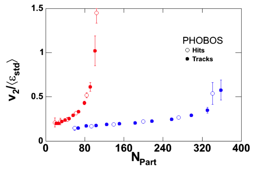

It was noticed in Ref. [30] that in collisions of heavy nuclei the fluctuations in the eccentricity can be well described by a two-dimensional Gaussian with the same width in both directions:
| (45) |
where , , and . What is not trivial is that for such Gaussian fluctuations the higher order cumulant flow values () are not only insensitive to nonflow but also to eccentricity fluctuations. All of the higher cumulants are exactly equal to , the flow projected onto the reaction plane. At the same time, the participant plane flow become unmeasurable because flow fluctuations can not be separated from nonflow contributions by means of correlation measurements. See Ref. [42].
The fact that higher order cumulants of eccentricity are very close to the “standard” values was initially observed in numerical calculations [34], and as an approximate result in Ref. [31]. Numerically, deviations were observed only for lighter (Cu+Cu) systems, which were traced to a break in the Gaussian approximation [41]. Experimentally, this question can be addressed by comparing the values of higher order cumulant flow with results obtained with the first harmonic reaction plane determined by spectator neutrons (at RHIC with the help of Zero Degree Calorimeters). Note also that using the first harmonic reaction plane one can also address the validity of the Gaussian approximation by direct fluctuation measurements [101].
An important conclusion from that study of eccentricity fluctuations was that in most cases the measurements of higher order cumulant flow values provide elliptic flow relative to the reaction plane and not the participant plane. Similarly, the same value is given by several other methods, such as Lee-Yang Zeros, Bessel Transform, and the fit to q-distribution. This greatly simplifies the comparison of hydrodynamic calculations to data, as it says that in such calculations one should not worry about how to take into account fluctuations in the initial eccentricity (which is a non-trivial task) but just compare to the “right” measurement, , e.g. . This understanding also explains some earlier calculations with the uRQMD model [102, 103]. There, it was shown that using higher cumulants and/or the LYZ method one indeed can measure elliptic flow very well, but it was not at all clear why there was no trace of the effects of flow fluctuations, which were expected in this model.
Unfortunately this progress in understanding the nature of fluctuations does not help in resolving the problem of measuring flow fluctuations and nonflow. Strictly speaking, to separate those effects one is required to make assumptions. Most often, the azimuthal correlations between particles with large rapidity separation are used to suppress nonflow contributions. The problem with this method is that there are no reliable estimates of how well they suppresses nonflow and also how much the flow fluctuations (in this case correlations) change after imposing such a cut.
At the QM’08 conference the PHOBOS [104] and STAR [105] collaborations have presented their revised (compared to QM’06) results on flow fluctuations. These results are in good agreement, see Figs. 29, 29. In Ref. [105] a conservative approach is taken and only upper limits on fluctuations are reported. The PHOBOS Collaboration uses estimates of nonflow effects from correlations with large rapidity separation and reports a more restrictive range for fluctuations. Both agree that the current measurements exhaust the (nucleon) eccentricity values obtained in the MC Glauber model and in this sense somewhat favor models which predict smaller relative fluctuations, such as the CGC model or a MC Glauber model taking into account constituent quark substructure.


(Pseudo)rapidity dependence
The measured pseudorapidity dependence of elliptic flow is shown in Figs. 31–33. In general exhibits a dependence, with a maximum at mid-rapidity and falls off in the fragmentation regions. Such behavior would find a natural explanation in the LDL. Collision energy and nuclear size dependence of , Fig. 31, would also roughly agree with scaling proportional to the charged particle density. For 10–40% centrality Fig. 31 compares the PHOBOS and STAR results. It appears that using the Lee-Yang Zeros method has about the same effect as having a pseudorapidity gap.


Similar to the limiting fragmentation picture of charged particle density, elliptic flow exhibits the same behavior. Figure 33 shows how the PHOBOS data plotted against , where is the projectile rapidity, collapses on the universal curve in the fragmentation region. The original hydrodynamic models predictions for are far from the data (see the solid curve in Fig. 33). Note that 3d hydrodynamic calculations are computationally difficult and the dependence of the initial conditions on rapidity is far from being known. In all calculations so far a boost-invariant initial geometry is assumed. Adding a cascade hadronic afterburner greatly improves agreement with data (see Fig. 33) similar to the integral flow discussed above (Figs. 21 and 23).


Low region: mass splitting
For charged hadrons, shown in Fig. 24, the elliptic flow increases almost linearly as a function of reaching values of about 0.15 at large . At low transverse momenta, the dependence is well described by hydrodynamics.
As explained in section 3.1 in a (locally) thermalized system, like in hydrodynamics, the interplay of radial expansion and anisotropic flow should lead to a specific dependence of the differential flow on the mass of the particle [51, 52, 108]. Figure 34 shows as function of transverse momentum for two particle species. As expected, at low the elliptic flow clearly depends on the mass of the particle with at a fixed decreasing with increasing mass. The hydrodynamic model calculations of for pions and (anti-)protons in Fig. 34 are performed for two equations of state: the full curves are for an EoS which incorporates the effect of a phase transition from a QGP to a hadron gas, the dashed curves are for a hadronic EoS without phase transition. The hydro calculations clearly predict the observed behavior rather well with a better description of the measurements provided by the EoS incorporating a phase transition. For the pions the effect of a phase transition is less pronounced compared to the protons. The lighter particles are more affected by the temperature, thus less sensitive to the collective flow velocity and vice versa for the heavier particles. One should not, however, conclude from the good fit of the ideal hydro calculations to the data in Fig. 34 that the EoS which includes the phase transition is the only allowed EoS. To draw conclusions about the EoS one first has to better understand the initial conditions [77, 78, 79, 80], has to have a more realistic description of the phase transition [109], and quantify the effects of viscous corrections [87, 88, 89, 90, 91, 92].
Figure 35 shows that the elliptic flow of the different mass particles at low can be characterized rather well by a common set of four freeze-out parameters: the temperature, the mean radial flow velocity, the azimuthal dependence of the radial flow velocity and the source deformation [35]. In hydrodynamics, these parameters are not independent since they are related by the initial conditions and the equation of state. This also explains why differential flow for heavier particles is sensitive to the EoS.
The four parameter blast-wave model fit, to the extent that it provides an accurate description of the system at freeze-out, has an advantage over hydrodynamic and cascade models in that it allows extraction of these freeze-out parameters without knowledge of the systems history before freeze-out. The blast-wave parameters obtained by fitting the pion and (anti-)proton in Ref. [35] also described the later obtained measurements of for the heavier and Cascade particles, as can be seen in Fig. 35. In addition, the obtained parameter which describes the source deformation was later confirmed also by azimuthally sensitive femtoscopy measurements [111].
In ideal hydrodynamics the mass ordering in persists up to large , although less pronounced because the of the different particles start to approach each other. It is seen that at higher the measurements start to deviate significantly from hydrodynamics for all particle species, and that the observed of the heavier baryons is larger than that of the lighter mesons. This mass dependence is the reverse of the behavior observed at low . This is not expected for hadrons in hydrodynamics and is also not expected if the is caused by parton energy loss (in the latter case there would be, to first order, no dependence on particle type). An elegant explanation of the unexpected particle type dependence and magnitude of at large is provided by the coalescence picture [61, 112] and is discussed in Sec. 3.3.
Constituent quark number scaling
Elliptic flow of identified particles measured in Au+Au collisions at RHIC exhibits a remarkable scaling with the number of constituent quarks – an apparent dependence of hadron elliptic flow at intermediate transverse momenta, GeV/, on the number of constituent quarks in the hadron. This observation is of particular interest and importance, as it indicates that the system is in a deconfined stage. In a more general sense, it appears that high energy nuclear collisions provide a window of opportunity to prove that hadron production indeed happens via the constituent quark phase. It has been noticed in Ref. [61] that if hadrons are formed via coalescence of the constituent quarks then there should be a region in the transverse momentum space where particle yield would be proportional to the quark density to the power equal to the number of constituent quarks in the produced hadron, 2 for mesons and 3 for baryons. Besides other important consequences, such as enhanced relative production of baryons in this transverse momentum region, this picture leads to the constituent quark scaling of elliptic flow, , where is the number of constituent quarks in the hadron [61, 112]. Figure 37 shows this scaling holds with good accuracy. Note that while the scaling itself is limited to a specific region in transverse momentum, the coalescence mechanism can be valid at all smaller momenta. The reason for the scaling violation at lower momenta might be that the equations used to describe coalescence break down. For identified particles the scaling for mesons and baryons is based on the equations
| (46) |
which are valid only if the probability of coalescence is relatively low. At low transverse momentum, where most of the quarks hadronize via coalescence these equations break unitarity. Note that according to these equations, the hadron yield scales with power 2 or 3 of the quark density. For a discussion of the particle spectra calculations and further development of the coalescence picture we refer to the review in Ref. [113].
In this picture the quantity is interpreted as the elliptic flow of constituent quarks. This means deconfinement – as the constituent quarks must be in a deconfined phase in order to be freely “reshuffled” into final hadrons. This could be the first, and very strong argument for an observation of deconfined matter at RHIC. The meson is an interesting test of constituent quark scaling. It has the mass of a proton but contains only two quarks. Figure 37 shows that its values are consistent with the two-quark curve thereby supporting the quark picture.

Figure 38 shows that plotting vs transverse kinetic energy , where , results in the formation of distinct branches for mesons and baryons. Scaling with the number of constituent quarks then coalesces the two branches into one curve. At the moment there is no agreement on the reason for such a universal scaling except that re-plotting the data vs transverse kinetic energy to some extent compensates for the effect of radial flow (see the discussion in section 3.1). But we mention that transverse kinetic energy scaling is an approximation to a more general scaling found in the Buda-Lund model [117]. Also, a quark recombination model based on q-qbar resonance interactions may account for this phenomenon[118].
A detailed study of necessary conditions for the quark-number scaling to be valid has been performed by Pratt and Pal [119]. Two limiting possibilities are illustrated in Fig. 40, where the particles (quarks) of a given velocity are represented by arrows. In case (a) the effective volumes of the right-moving and upward-moving particles are the same but the right-moving particles have a larger phase space density. In case (b) the densities are the same but the volumes differ. Both cases correspond to the same quark , but only case (a) would lead to the quark-number scaling. Based on this analysis one might conclude that constituent quark scaling contradicts local thermalization and freeze-out at a constant phase-space density. Even if true, this does not diminish the validity of the conclusion on deconfinement, but points to a very interesting possibility that the system created in the heavy ion collision can be in a deconfined but not completely thermalized state. It also does not exclude the possibility that thermalization happens only for lower transverse momenta.

The success of quark coalescence as a hadronization mechanism in describing particle production at intermediate transverse momenta hints on the importance of the constituent quark dynamics in the evolution of the system in general. Recall that the transport models [66, 120] in their standard configuration fail to describe the strong increase of elliptic flow with energy. They have to significantly increase the parton transport cross section or the matter density in order to reach the experimental values. On the other hand if one looks carefully into what particular parameters are required in order to describe the data, an interesting picture emerges: the density and partonic cross sections are just what one would expect for a system of constituent quarks. For example, Fig. 40 shows a comparison of the experimental data to the AMPT [66] model calculations in the so-called melted string scenario. The main assumption of this scenario is that the total number of partons in the system equals the number of constituent quarks in the produced hadrons, exactly what one would use for a model based on the picture of a system of constituent quarks. Note that the model describes the data best with a cross section of about 5 mb, which is what one expects for constituent quarks. Similar conclusion can be drawn from Fig. 41 which shows the results of calculations in the MPC [120] model, using as a reference the standard HIJING gluon density ( for central Au+Au collisions) and a cross section of about 2 mb. Again, rescaling the parton density to that corresponding to the total number of quarks in the final hadrons and increasing the cross section to 5–6 mb one would achieve a reasonable description of the data.

Figure 42 shows the comparison of the experimental data on to calculations in the low density limit [121]. According to the equations of the LDL, saturates at transverse momenta about a few times the particle mass. The calculations, shown by a dashed curve, exhibits this very behavior as first exhausting flow of pions and then at higher that of protons. Indeed the results do not resemble the data. But it is clear that similar calculations performed with masses of the constituent quarks (a few times that of the pion) taken together with coalescence enhancement at intermediate transverse momenta could well be consistent with the data. (See also the upper panel in Fig. 37 and the right panel of Fig. 38, which can be considered as of constituent quarks.) This again strongly advocates for a major role of constituent quark dynamics in the system evolution.
Note that, in principle, hadronization always, even in small systems and at lower energies, occurs via constituent quark coalescence. The importance of the observation of quark number scaling in elliptic flow, is that it constitutes deconfinement – “free” kinetics of quarks in the system. In this sense this scaling is a signature of deconfinement and should be violated under conditions when deconfinement does not happen.
High region
Elliptic anisotropy at high transverse momenta is an interesting observable as it is believed that it reflects the path length dependence of high parton energy loss [122]. At sufficiently high transverse momentum in Au+Au collisions, hadron yields are thought to contain a significant fraction originating from the fragmentation of high energy partons, resulting from initial hard scatterings. Calculations based on perturbative QCD (pQCD) predict that high energy partons traversing nuclear matter lose energy through induced gluon radiation [123, 124]. The energy loss (jet quenching) is expected to depend strongly on the color charge density of the created system and the traversed path length of the propagating parton. In non-central heavy-ion collisions, the geometrical overlap region has an almond shape in the transverse plane, with its short axis in the reaction plane. Depending on the azimuthal emission angle, partons traversing such a system, on average, experience different path lengths and therefore different energy loss. This mechanism introduces an azimuthal anisotropy in particle production at high transverse momenta [122, 125, 126].
The dashed lines in Fig. 43 show the first quantitative theory predictions based on energy-loss calculations in a static medium [127] and are compared to STAR measurements [128]. However, as was discussed in the previous section, it was realized that in the range of GeV/ hadron yields might not dominantly originate from the fragmentation of high energy partons but are instead mostly produced by quark coalescence. Therefore in order to compare to predictions of parton energy loss has to be measured above GeV/. Unfortunately nonflow contributions which at low are modest are significant at high . In fact nonflow might even start to dominate the measured two-particle azimuthal correlations at high which complicates making reliable measurements.
Assuming that there is no anisotropic flow in pp and dAu collisions one can estimate the contribution from nonflow by comparing the two- particle azimuthal correlation in these systems with the azimuthal correlation in AuAu. Figure 44 shows the measured azimuthal correlation as a function of transverse momentum in pp and dAu collisions as well as for three different centralities in AuAu. The two-particle azimuthal correlation shown is defined in Eq. (31). It is seen that the magnitude of the azimuthal correlations in pp, dAu and very peripheral AuAu is comparable over the complete measured transverse momentum range. This indicates that in peripheral AuAu collisions nonflow correlations are the dominant contribution. On the other hand, for mid-central and central AuAu collisions at low and intermediate the observed azimuthal correlation is much stronger than in pp and dAu as is expected in the presence of strong anisotropic flow. However, at high , even for these mid-central and central AuAu collisions, the two-particle azimuthal correlation are again dominated by the correlations already seen in pp and dAu. The remaining difference in the azimuthal correlation at high can be used to estimate the elliptic flow, which is done in Refs. [26, 129].
Instead of using pp and dAu collisions as a reference for nonflow, the large data sample obtained at RHIC in Au+Au collisions at GeV now also allows for calculating the anisotropic flow coefficients up to GeV/ using higher order cumulants. Figure 45 shows the obtained using the order cumulant, and the values are compared to the obtained using the event plane method and the 2-particle cumulant. The values from the event plane method and 2-particle cumulant exhibit the same large values at high as seen in Fig. 44. The obtained from the order cumulant method at high is at least a factor of two smaller, however still significant. These values can be compared to model calculations to better constrain the mechanism responsible for parton energy loss.
Another approach to reduce nonflow is to make sure that there is a large gap in rapidity between the particles used to determine the event plane and the particles used to calculate the elliptic flow. In STAR, in addition to the ZDCs, the Forward TPCs (FTPCs) which are located at can be used for this [131]. Figure 46 left compares the measured at midrapidity () from the 2-particle cumulant and from the event plane method using the STAR FTPCs. As was already observed, the nonflow (here the difference between and ) is significant above 2 GeV/ and becomes large above 6 GeV/. Assuming that the nonflow is completely removed with the difference between from Fig. 45 and in Fig. 46 left shows the difference between in the reaction plane and in the participant plane with fluctuations. However, because the curves still turn up at very high , there is probably still some nonflow even with the event plane determined in the FTPCs.
Clearly for mid-central collisions in AuAu the nonflow contribution at high is already significant. In case of CuCu, i.e. a smaller system, the elliptic flow for the same midcentral collisions is expected to be smaller while the relative nonflow contribution is expected to be larger. Figure 46 right shows the measured in CuCu with the order cumulant and with the event plane method using the STAR FTPCs [131]. It is seen that the in CuCu obtained from the two-particle cumulant method at intermediate (4–12 GeV/) is even larger than in AuAu. In contrast the in CuCu obtained from the event plane method using the FTPCs is smaller than in AuAu over almost the whole range. This confirms that in CuCu indeed the is smaller than in AuAu while the nonflow effects are larger. Even though statistical uncertainties are large for above 6 GeV/ the transition to again increasing values of might indicate that a rapidity gap of is still not large enough to remove all nonflow in CuCu.
Rare probes
Elliptic flow of heavy flavor and direct photons, often called by the common name rare probes, attract significant attention as they provide important additional information about the dynamics and properties of the sQGP created in heavy ion collisions. Heavy flavor elliptic flow is studied either directly or via single electrons from semi-leptonic decays.

Elliptic flow of hadrons containing charm or bottom quark(s) provide direct information on the collectivity of heavy flavor quarks in the deconfined stage. So far there exist data from PHENIX on flow of single electrons and very limited data on flow of . Simulations show that for 2–3 GeV/ most electrons are from semi-leptonic decays of charm and bottom, and at 5–8 GeV/ it could be dominated by bottom decays. At such transverse momentum, electrons to a large degree preserve the direction of heavy flavor mesons and thus can be studied to evaluate the elliptic flow of charm or bottom quarks. In a simple coalescence picture [132] the elliptic flow of charm hadrons is a combination of the elliptic flow of corresponding quarks taken at appropriate transverse momentum (roughly shared in proportion to the quark masses). It appearers that, for example, charm meson elliptic flow at transverse momentum of about 3 GeV/ may differ more than a factor of 2 depending on whether charm quarks participate in collective flow [132].


PHENIX measurements [133, 134], shown in Fig. 47, indicate that heavy quarks flow at the same level as light ones. From this measurement (combined with heavy flavor electron spectra) PHENIX derives an upper limit on viscosity , confirming that the system behaves as a near perfect liquid. Results on elliptic flow of have just started to appear [134], and in spite of large errors they immediately attract attention as they are largely consistent with out-of-plane elliptic flow, thus possibly indicating strong effects of radial flow [136], as discussed in Sec. 3.1.
Elliptic flow of direct photons has a very rich physics as there have been identified several mechanisms which lead to significant elliptic flow. The most important are: (i) thermal photons, (ii) photons from high parton fragmentation (in vacuum), (iii) bremsstrahlung and “jet conversion” photons from fast partons propagating inside the medium. Thermal photons originate both in QGP and hadronic phases. Calculations [137] show that even though the QGP phase is short due to higher temperature, it gives the largest contribution to photons at intermediate transverse momenta (see Fig. 48). High photons come from hard parton-parton scattering with subsequent usual fragmentation (leading to positive ) or to bremsstrahlung, which is stronger out-of-plane leading to negative . The combination of all these effects results in a rather complicated picture (see Fig. 49). There is hope that with large statistics different mechanisms could be separated with different isolation cuts. Finally, note that the mechanism, similar to that of “jet conversion” could also lead to an enrichment of jet fragments with some rare particles (including strangeness content). It would lead to the corresponding negative contribution to the elliptic flow of that particle [138].
3.4 Higher harmonics
The higher harmonics give more detail about the shape of the azimuthal anisotropy. Values for and are shown in Fig. 50 [24]. The values appear to scale as as shown in Fig. 50. For identified particles in Fig. 51, appears to have the same scaling as with transverse kinetic energy , but vs it seems to scale as the square of the number of constituent quarks [140] as one would guess because [24]. The proportionality constant can be seen in Fig. 52. For ideal hydro this ratio should be [108] at high . Boltzmann calculations indicate that a finite Knudsen number [141] is needed to describe the deviation of the data from non-viscous hydro.


4 Conclusion and outlook
The wealth of information obtained recently in the area of anisotropic flow is far from being fully explored. The theoretical understanding of the experimental data is rapidly developing and greatly contributes to the overall picture of heavy ion collisions dynamics as well as the properties of the new state of matter, sQGP. Unfortunately, we have not been able to discuss many other important measurements related to the event anisotropy, such as azimuthally sensitive identical and non-identical particle femtoscopic measurements [143, 144] (for a recent review, see Ref. [145]) or two particle correlations relative to the reaction plane [129, 146].
The next years promise to bring new very important data which will shed more light on quite a few remaining questions. The most important developments we expect are in the following directions: (i) upgrade of RHIC detectors will give more precise information on identified particle anisotropic flow, (ii) beam energy scan at RHIC will allow looking very carefully in the region where critical phenomena are expected (e.g. color percolation, critical point), in particular to look for any non-monotonic behavior or scaling violation in the plot, (iii) U+U collisions at RHIC, (iv) and, of course, the first data at LHC is eagerly expected to answer what happens at higher beam energies.
The main interest in the RHIC beam energy scan is the search for the QCD critical point. The scan would cover the energy region from top AGS energies, over the CERN SPS energies, and higher. In terms of anisotropic flow the major observables to watch would be a possible non-smooth behavior in the dependence on particle density [69], a possible disappearance of constituent quark number scaling, and the “collapse” of directed flow [147] (see Fig. 54). RHIC also has plans to extend its reach in terms of energy density using uranium beams. From the first estimates and ideas of using uranium beams we now have detailed simulations [148] of such collisions with methods developed for selection of the desired geometry of the collision.
The predictions for the LHC are rather uncertain, though most researchers agree that elliptic flow will continue to increase [149], partially due to the relatively smaller contribution of viscous effects. Simple extrapolations [150, 151] in Fig. 54 of the collision energy dependence of look rather reliable. Theoretical calculations predict significantly smaller, thought still finite, viscous effect at LHC energies. One can see it in Fig. 21 which shows evolution with particle density up to LHC energies in 3d-hydro+cascade approach. Note that there exist some calculations predicting a decrease of the elliptic flow [152]. Another important observation is an increase in mass dependence (splitting) of due to a strong increase of radial flow.
In summary, we have had very exciting years of anisotropic flow study, which greatly enriched our understanding of ultra-relativistic nuclear collisions and multi-particle production in general. We are looking forward to more new physics with RHIC and LHC.

5 Acknowledgments
We thank all our colleagues for numerous discussions on many of the topics discussed in this review. We thank our colleagues in STAR for permission to use some of our text from published STAR papers. We appreciate comments on the paper from Ante Bilandzic, Pasi Huovinen, Claude Pruneau, Ralf Rapp, and Gang Wang. This work was supported in part by FOM and NWO of the Netherlands, and the HENP Divisions of the Office of Science of the US Department of Energy under Contract Numbers DE-AC02-05CH11231 and DE-FG02-92ER40713.
References
- (1) J. Y. Ollitrault, Phys. Rev. D 46, 229 (1992).
- (2) J. Barrette et al. [E877 Collaboration], Phys. Rev. Lett. 73, 2532 (1994) [arXiv:hep-ex/9405003].
- (3) J. Barrette et al. [E877 Collaboration], Phys. Rev. C 55, 1420 (1997) [Erratum-ibid. C 56, 2336 (1997)] [arXiv:nucl-ex/9610006].
- (4) C. Alt et al. [NA49 Collaboration], Phys. Rev. C 68, 034903 (2003) [arXiv:nucl-ex/0303001].
- (5) K. H. Ackermann et al. [STAR Collaboration], Phys. Rev. Lett. 86, 402 (2001) [arXiv:nucl-ex/0009011].
- (6) K. G. Boreskov, A. B. Kaidalov and O. V. Kancheli, arXiv:0809.0625 [hep-ph].
- (7) B. Z. Kopeliovich, A. H. Rezaeian and I. Schmidt, arXiv:0809.4327 [hep-ph].
- (8) D. Teaney and R. Venugopalan, Phys. Lett. B 539, 53 (2002) [arXiv:hep-ph/0203208].
- (9) A. Krasnitz, Y. Nara and R. Venugopalan, Phys. Lett. B 554, 21 (2003) [arXiv:hep-ph/0204361].
- (10) W. Reisdorf and H. G. Ritter, Ann. Rev. Nucl. Part. Sci. 47, 663 (1997).
- (11) N. Herrmann, J. P. Wessels and T. Wienold, Ann. Rev. Nucl. Part. Sci. 49, 581 (1999).
- (12) S. Voloshin and Y. Zhang, Z. Phys. C 70, 665 (1996) [arXiv:hep-ph/9407282].
- (13) J. Y. Ollitrault, arXiv:nucl-ex/9711003.
- (14) J. Y. Ollitrault, Nucl. Phys. A 638, 195 (1998) [arXiv:nucl-ex/9802005].
- (15) A. M. Poskanzer and S. A. Voloshin, Phys. Rev. C 58, 1671 (1998) [arXiv:nucl-ex/9805001].
- (16) P. Danielewicz and G. Odyniec, nucleusÐnucleus collisions” Phys. Lett. B 157, 146 (1985).
- (17) J. Y. Ollitrault, Phys. Rev. D 48, 1132 (1993) [arXiv:hep-ph/9303247].
- (18) N. Borghini, P. M. Dinh and J. Y. Ollitrault, Phys. Rev. C 64, 054901 (2001) [arXiv:nucl-th/0105040].
- (19) I. Selyuzhenkov and S. Voloshin, Phys. Rev. C 77, 034904 (2008) [arXiv:0707.4672 [nucl-th]].
- (20) S. Wang et al., Phys. Rev. C 44, 1091 (1991).
- (21) C. Adler et al. [STAR Collaboration], Phys. Rev. C 66, 034904 (2002) [arXiv:nucl-ex/0206001].
- (22) N. Borghini, P. M. Dinh and J. Y. Ollitrault, arXiv:nucl-ex/0110016.
- (23) B. I. Abelev et al. [STAR Collaboration], Phys. Rev. C 77, 054901 (2008) [arXiv:0801.3466 [nucl-ex]].
- (24) J. Adams et al. [STAR Collaboration], Phys. Rev. Lett. 92, 062301 (2004) [arXiv:nucl-ex/0310029].
- (25) N. Borghini, P. M. Dinh and J. Y. Ollitrault, Phys. Rev. C 66, 014905 (2002) [arXiv:nucl-th/0204017].
- (26) J. Adams et al. [STAR Collaboration], Phys. Rev. C 72, 014904 (2005) [arXiv:nucl-ex/0409033].
- (27) J. Y. Ollitrault, Nucl. Phys. A 590, 561C (1995).
- (28) R. S. Bhalerao, N. Borghini and J. Y. Ollitrault, Nucl. Phys. A 727, 373 (2003) [arXiv:nucl-th/0310016].
- (29) N. Borghini, R. S. Bhalerao and J. Y. Ollitrault, J. Phys. G 30, S1213 (2004) [arXiv:nucl-th/0402053].
- (30) S. A. Voloshin, A. M. Poskanzer, A. Tang and G. Wang, Phys. Lett. B 659, 537 (2008) [arXiv:0708.0800 [nucl-th]].
- (31) R. S. Bhalerao and J. Y. Ollitrault, Phys. Lett. B 641, 260 (2006) [arXiv:nucl-th/0607009].
- (32) A. Bilandzic, N. van der Kolk, J. Y. Ollitrault and R. Snellings, arXiv:0801.3915 [nucl-ex].
- (33) N. Borghini and J. Y. Ollitrault, Nucl. Phys. A 742, 130 (2004) [arXiv:nucl-th/0404087].
- (34) S. A. Voloshin, arXiv:nucl-th/0606022.
- (35) C. Adler et al. [STAR Collaboration], Phys. Rev. Lett. 87, 182301 (2001) [arXiv:nucl-ex/0107003].
- (36) N. Borghini, P. M. Dinh and J. Y. Ollitrault, Phys. Rev. C 62, 034902 (2000) [arXiv:nucl-th/0004026].
- (37) P. M. Dinh, N. Borghini and J. Y. Ollitrault, Phys. Lett. B 477, 51 (2000) [arXiv:nucl-th/9912013].
- (38) ÊS. A. Voloshin, ÊÊÊPhys. Lett. ÊB 632, 490 (2006) Ê[arXiv:nucl-th/0312065]. Ê
- (39) T. A. Trainor and D. T. Kettler, Int. J. Mod. Phys. E 17 (2008) 1219 [arXiv:0704.1674 [hep-ph]].
- (40) N. Borghini, P. M. Dinh, J. Y. Ollitrault, A. M. Poskanzer and S. A. Voloshin, Phys. Rev. C 66, 014901 (2002) [arXiv:nucl-th/0202013].
- (41) B. Alver et al., Phys. Rev. C 77, 014906 (2008) [arXiv:0711.3724 [nucl-ex]].
- (42) J.-Y. Ollitrault, A.M. Poskanzer, S.A. Voloshin, in preparation, 2008.
- (43) R. Stock, private communication, 2008.
- (44) W. Broniowski, M. Chojnacki, W. Florkowski and A. Kisiel, Phys. Rev. Lett. 101, 022301 (2008) [arXiv:0801.4361 [nucl-th]].
- (45) M. Gyulassy, Yu. M. Sinyukov, I. Karpenko and A. V. Nazarenko, Braz. J. Phys. 37, 1031 (2007).
- (46) F. Becattini, F. Piccinini and J. Rizzo, Phys. Rev. C 77, 024906 (2008) [arXiv:0711.1253 [nucl-th]].
- (47) S. M. Troshin and N. E. Tyurin, arXiv:0709.4090 [hep-ph].
- (48) G. Wang, J. Phys. G 34, S1093 (2007) [arXiv:nucl-ex/0701045].
- (49) L. P. Csernai, J. I. Kapusta and L. D. McLerran, J. Phys. G 32, S115 (2006).
- (50) R. J. M. Snellings, H. Sorge, S. A. Voloshin, F. Q. Wang and N. Xu, Phys. Rev. Lett. 84, 2803 (2000) [arXiv:nucl-ex/9908001].
- (51) S. A. Voloshin, Phys. Rev. C 55, 1630 (1997) [arXiv:nucl-th/9611038].
- (52) P. Huovinen, P. F. Kolb, U. W. Heinz, P. V. Ruuskanen and S. A. Voloshin, Phys. Lett. B 503, 58 (2001) [arXiv:hep-ph/0101136].
- (53) F. Retiere and M. A. Lisa, Phys. Rev. C 70, 044907 (2004) [arXiv:nucl-th/0312024].
- (54) J. Barrette et al. [E877 Collaboration], Phys. Rev. C 56, 3254 (1997) [arXiv:nucl-ex/9707002].
- (55) A. Franz [PHENIX Collaboration], arXiv:0805.1718 [nucl-ex].
- (56) H. d. Liu, J. Phys. G 34, S1087 (2007) [arXiv:nucl-ex/0701057].
- (57) S. Voloshin et al. [The E877 Collaboration], Nucl. Phys. A 638, 455C (1998) [arXiv:nucl-ex/9802001].
- (58) J. Barrette et al. [E877 collaboration], Phys. Rev. C 59, 884 (1999) [arXiv:nucl-ex/9805006].
- (59) S. Afanasiev et al. [PHENIX Collaboration], Phys. Rev. Lett. 99, 052301 (2007) [arXiv:nucl-ex/0703024].
- (60) J. Adams et al. [STAR Collaboration], Phys. Rev. C 71, 064902 (2005) [arXiv:nucl-ex/0412019].
- (61) S. A. Voloshin, Nucl. Phys. A 715, 379 (2003) [arXiv:nucl-ex/0210014].
- (62) J. Brachmann et al., Phys. Rev. C 61, 024909 (2000) [arXiv:nucl-th/9908010].
- (63) L. P. Csernai and D. Rohrich, Phys. Lett. B 458, 454 (1999) [arXiv:nucl-th/9908034].
- (64) L. P. Csernai et al., Acta Phys. Hung. A 22, 181 (2005) [arXiv:hep-ph/0405277].
- (65) B. I. Abelev et al. [STAR Collaboration], arXiv:0807.1518 [nucl-ex].
- (66) Z. w. Lin and C. M. Ko, Phys. Rev. C 65, 034904 (2002) [arXiv:nucl-th/0108039].
- (67) A. Wetzler, private communication (2005).
- (68) H. Heiselberg and A. M. Levy, Phys. Rev. C 59, 2716 (1999) [arXiv:nucl-th/9812034].
- (69) S. A. Voloshin and A. M. Poskanzer, Phys. Lett. B 474, 27 (2000) [arXiv:nucl-th/9906075].
- (70) H. Sorge, Phys. Rev. Lett. 82, 2048 (1999) [arXiv:nucl-th/9812057].
- (71) P. F. Kolb, J. Sollfrank and U. W. Heinz, Phys. Rev. C 62, 054909 (2000) [arXiv:hep-ph/0006129].
- (72) H. Satz, Nucl. Phys. A 715, 3 (2003) [arXiv:hep-ph/0209181].
- (73) M. Gyulassy and L. McLerran, Nucl. Phys. A 750, 30 (2005) [arXiv:nucl-th/0405013].
- (74) P. Kovtun, D. T. Son and A. O. Starinets, Phys. Rev. Lett. 94, 111601 (2005) [arXiv:hep-th/0405231].
- (75) T. Hirano, Prog. Theor. Phys. Suppl. 168, 347 (2007) [arXiv:0704.1699 [nucl-th]].
- (76) P. Huovinen, arXiv:0710.4379 [nucl-th].
- (77) T. Hirano, U. W. Heinz, D. Kharzeev, R. Lacey and Y. Nara, Phys. Lett. B 636, 299 (2006) [arXiv:nucl-th/0511046].
- (78) H. J. Drescher, A. Dumitru, A. Hayashigaki and Y. Nara, Phys. Rev. C 74, 044905 (2006) [arXiv:nucl-th/0605012].
- (79) H. J. Drescher and Y. Nara, Phys. Rev. C 76, 041903 (2007) [arXiv:0707.0249 [nucl-th]].
- (80) T. Lappi and R. Venugopalan, Phys. Rev. C 74, 054905 (2006) [arXiv:nucl-th/0609021].
- (81) R. S. Bhalerao, J. P. Blaizot, N. Borghini and J. Y. Ollitrault, Phys. Lett. B 627, 49 (2005) [arXiv:nucl-th/0508009].
- (82) H. J. Drescher, A. Dumitru, C. Gombeaud and J. Y. Ollitrault, Phys. Rev. C 76, 024905 (2007) [arXiv:0704.3553 [nucl-th]].
- (83) A. Tang [for the STAR Collaboration], arXiv:0808.2144 [nucl-ex].
- (84) D. Teaney, J. Lauret and E. V. Shuryak, arXiv:nucl-th/0110037.
- (85) C. Nonaka and S. A. Bass, Phys. Rev. C 75, 014902 (2007) [arXiv:nucl-th/0607018].
- (86) D. Teaney, J. Lauret and E. V. Shuryak, Phys. Rev. Lett. 86, 4783 (2001) [arXiv:nucl-th/0011058].
- (87) D. Teaney, Phys. Rev. C 68, 034913 (2003) [arXiv:nucl-th/0301099].
- (88) P. Romatschke and U. Romatschke, Phys. Rev. Lett. 99, 172301 (2007) [arXiv:0706.1522 [nucl-th]].
- (89) M. Luzum and P. Romatschke, Phys. Rev. C 78, 034915 (2008) [arXiv:0804.4015 [nucl-th]].
- (90) H. Song and U. W. Heinz, Phys. Lett. B 658, 279 (2008) [arXiv:0709.0742 [nucl-th]].
- (91) H. Song and U. W. Heinz, Phys. Rev. C 77, 064901 (2008) [arXiv:0712.3715 [nucl-th]].
- (92) K. Dusling and D. Teaney, Phys. Rev. C 77, 034905 (2008) [arXiv:0710.5932 [nucl-th]].
- (93) H. Song and U. W. Heinz, Phys. Rev. C 78, 024902 (2008) [arXiv:0805.1756 [nucl-th]].
- (94) Z. Xu, C. Greiner and H. Stocker, Phys. Rev. Lett. 101, 082302 (2008) [arXiv:0711.0961 [nucl-th]].
- (95) C. E. Aguiar, Y. Hama, T. Kodama and T. Osada, Nucl. Phys. A 698, 639 (2002) [arXiv:hep-ph/0106266].
- (96) M. Miller and R. Snellings, arXiv:nucl-ex/0312008.
- (97) S. Manly et al. [PHOBOS Collaboration], Nucl. Phys. A 774, 523 (2006) [arXiv:nucl-ex/0510031].
- (98) W. Broniowski, P. Bozek and M. Rybczynski, Phys. Rev. C 76, 054905 (2007) [arXiv:0706.4266 [nucl-th]].
- (99) R. Andrade, F. Grassi, Y. Hama, T. Kodama and O. . J. Socolowski, Phys. Rev. Lett. 97, 202302 (2006) [arXiv:nucl-th/0608067].
- (100) B. Alver et al. [PHOBOS Collaboration], Phys. Rev. Lett. 98, 242302 (2007) [arXiv:nucl-ex/0610037].
- (101) G. Wang, D. Keane, A. Tang and S. A. Voloshin, Phys. Rev. C 76, 024907 (2007) [arXiv:nucl-ex/0611001].
- (102) X. l. Zhu, M. Bleicher and H. Stoecker, Phys. Rev. C 72, 064911 (2005) [arXiv:nucl-th/0509081].
- (103) X. l. Zhu, M. Bleicher and H. Stoecker, J. Phys. G 32, 2181 (2006) [arXiv:nucl-th/0601049].
- (104) B. Alver et al. [PHOBOS Collaboration], arXiv:0804.4297 [nucl-ex].
- (105) P. Sorensen [STAR Collaboration], arXiv:0808.0356 [nucl-ex].
- (106) B. B. Back et al. [PHOBOS Collaboration], Phys. Rev. C 72, 051901 (2005) [arXiv:nucl-ex/0407012].
- (107) R. Snellings [STAR Collaboration and ALICE Collaboration], Eur. Phys. J. C 49, 87 (2007) [arXiv:nucl-ex/0610010].
- (108) N. Borghini and J. Y. Ollitrault, Phys. Lett. B 642, 227 (2006) [arXiv:nucl-th/0506045].
- (109) P. Huovinen, Nucl. Phys. A 761, 296 (2005) [arXiv:nucl-th/0505036].
- (110) R. Snellings, arXiv:nucl-ex/0310019.
- (111) J. Adams et al. [STAR Collaboration], Phys. Rev. Lett. 93, 012301 (2004) [arXiv:nucl-ex/0312009].
- (112) D. Molnar and S. A. Voloshin, Phys. Rev. Lett. 91, 092301 (2003) [arXiv:nucl-th/0302014].
- (113) R. J. Fries, V. Greco and P. Sorensen, arXiv:0807.4939 [nucl-th].
- (114) B. I. Abelev et al. [the STAR Collaboration], Phys. Rev. C 75, 054906 (2007) [arXiv:nucl-ex/0701010].
- (115) B. I. Abelev et al. [STAR Collaboration], Phys. Rev. Lett. 99, 112301 (2007) [arXiv:nucl-ex/0703033].
- (116) A. Adare et al. [PHENIX Collaboration], Phys. Rev. Lett. 98, 162301 (2007) [arXiv:nucl-ex/0608033].
- (117) M. Csanad et al., arXiv:nucl-th/0512078.
- (118) L. Ravagli, H. van Hees and R. Rapp, arXiv:0806.2055 [hep-ph].
- (119) S. Pratt and S. Pal, Nucl. Phys. A 749, 268 (2005) [Phys. Rev. C 71, 014905 (2005)] [arXiv:nucl-th/0409038].
- (120) D. Molnar and M. Gyulassy, Nucl. Phys. A 697, 495 (2002) [Erratum-ibid. A 703, 893 (2002)] [arXiv:nucl-th/0104073].
- (121) P. F. Kolb, P. Huovinen, U. W. Heinz and H. Heiselberg, Phys. Lett. B 500, 232 (2001) [arXiv:hep-ph/0012137].
- (122) R. J. M. Snellings, A. M. Poskanzer and S. A. Voloshin, arXiv:nucl-ex/9904003.
- (123) M. Gyulassy and M. Plumer, Phys. Lett. B 243, 432 (1990).
- (124) X. N. Wang and M. Gyulassy, Phys. Rev. Lett. 68, 1480 (1992).
- (125) X. N. Wang, Phys. Rev. C 63, 054902 (2001) [arXiv:nucl-th/0009019].
- (126) M. Gyulassy, I. Vitev, X. N. Wang and P. Huovinen, Phys. Lett. B 526, 301 (2002) [arXiv:nucl-th/0109063].
- (127) M. Gyulassy, I. Vitev and X. N. Wang, Phys. Rev. Lett. 86, 2537 (2001) [arXiv:nucl-th/0012092].
- (128) C. Adler et al. [STAR Collaboration], Phys. Rev. Lett. 90, 032301 (2003) [arXiv:nucl-ex/0206006].
- (129) J. Adams et al. [STAR Collaboration], Phys. Rev. Lett. 93, 252301 (2004) [arXiv:nucl-ex/0407007].
- (130) Yuting Bai, PhD Thesis, NIKHEF, Amsterdam, Netherlands
- (131) S. A. Voloshin [STAR Collaboration], J. Phys. G 34, S883 (2007) [arXiv:nucl-ex/0701038].
- (132) Z. w. Lin and D. Molnar, Phys. Rev. C 68, 044901 (2003) [arXiv:nucl-th/0304045].
- (133) S. S. Adler et al. [PHENIX Collaboration], Phys. Rev. C 72, 024901 (2005) [arXiv:nucl-ex/0502009].
- (134) T. C. Awes [PHENIX Collaboration], arXiv:0805.1636 [nucl-ex].
- (135) H. van Hees, V. Greco and R. Rapp, Phys. Rev. C 73, 034913 (2006) [arXiv:nucl-th/0508055].
- (136) D. Krieg and M. Bleicher, arXiv:0806.0736 [nucl-th].
- (137) R. Chatterjee, E. S. Frodermann, U. W. Heinz and D. K. Srivastava, Phys. Rev. Lett. 96, 202302 (2006) [arXiv:nucl-th/0511079].
- (138) W. Liu and R. J. Fries, arXiv:0805.3721 [nucl-th].
- (139) S. Turbide, C. Gale and R. J. Fries, Phys. Rev. Lett. 96, 032303 (2006) [arXiv:hep-ph/0508201].
- (140) S. Huang [PHENIX Collaboration], arXiv:0804.4864 [nucl-ex].
- (141) C. Gombeaud and J. Y. Ollitrault, Phys. Rev. C 77, 054904 (2008) [arXiv:nucl-th/0702075].
- (142) P. F. Kolb, L. W. Chen, V. Greco and C. M. Ko, Phys. Rev. C 69, 051901 (2004) [arXiv:nucl-th/0402049].
- (143) S. A. Voloshin and W. E. Cleland, Phys. Rev. C 53, 896 (1996) [arXiv:nucl-th/9509025];Phys. Rev. C 54, 3212 (1996) [arXiv:nucl-th/9606033].
- (144) S. Voloshin, R. Lednicky, S. Panitkin and N. Xu, Phys. Rev. Lett. 79, 4766 (1997) [arXiv:nucl-th/9708044].
- (145) M. A. Lisa, S. Pratt, R. Soltz and U. Wiedemann, Ann. Rev. Nucl. Part. Sci. 55, 357 (2005) [arXiv:nucl-ex/0505014].
- (146) J. Bielcikova, S. Esumi, K. Filimonov, S. Voloshin and J. P. Wurm, Phys. Rev. C 69, 021901 (2004) [arXiv:nucl-ex/0311007].
- (147) H. Stocker, arXiv:0710.5089 [hep-ph].
- (148) C. Nepali, G. I. Fai and D. Keane, Phys. Rev. C 76, 051902 (2007) [Erratum-ibid. C 76, 069903 (2007)] [arXiv:0709.1497 [hep-ph]].
- (149) N. Armesto et al., J. Phys. G 35, 054001 (2008) [arXiv:0711.0974 [hep-ph]].
- (150) W. Busza, J. Phys. G 35, 044040 (2008) [arXiv:0710.2293 [nucl-ex]].
- (151) N. Borghini and U. A. Wiedemann, J. Phys. G 35, 023001 (2008) [arXiv:0707.0564 [hep-ph]].
- (152) D. Krieg and M. Bleicher, arXiv:0708.3015 [nucl-th].