Cosmological Structure Formation under MOND: a new numerical solver for Poisson’s equation
Abstract
We present a novel solver for an analogue to Poisson’s equation in the framework of modified Newtonian dynamics (MOND). This equation is highly non-linear and hence standard codes based upon tree structures and/or FFT’s in general are not applicable; one needs to defer to multi-grid relaxation techniques. After a detailed description of the necessary modifications to the cosmological -body code AMIGA (formerly known as MLAPM) we utilize the new code to revisit the issue of cosmic structure formation under MOND. We find that the proper (numerical) integration of a MONDian Poisson’s equation has some noticable effects on the final results when compared against simulations of the same kind but based upon rather ad-hoc assumptions about the properties of the MONDian force field. Namely, we find that the large-scale structure evolution is faster in our revised MOND model leading to an even stronger clustering of galaxies, especially when compared to the standard CDM paradigm.
Keywords:
galaxy: formation – methods: -body simulations – cosmology: theory – dark matter – large scale structure of Universe1 Introduction
Modified Newtonian dynamics (MOND) was proposed by Milgrom (1983) as an alternative to Newtonian gravity to explain galactic dynamics without the need for dark matter. Although current cosmological observations point to the existence of vast amounts of non-baryonic dark matter in the Universe (Komatsu et al., 2008, e.g.), it remains interesting to explore other alternatives, especially as not all of the features of CDM models appear to match observational data (e.g., the “missing satellite problem” (Klypin et al., 1999; Moore et al., 1999) and the so-called “cusp-core crisis” (de Blok et al., 2003; Swaters et al., 2003, e.g.)). In that regards it appears important to look for tests able to discriminate between MOND and Newtonian gravity, especially in the context of cosmology now that there exist various relativistic formulation of the MOND theory (Bekenstein, 2004; Zhao, 2007; Zhao, 2008). However, progress in that field has been hampered by the fact that MOND is a non-linear theory making any analytical predictions as well as numerical simulations a tedious task. To date, only a few codes exist that actually solve the MONDian analogue to Poisson equation in a non-cosmological context (Brada & Milgrom, 1999; Nipoti et al., 2007; Tiret & Combes, 2007), none of which is publically available. We are augmenting this list by making available a new solver for the MONDian Poisson’s equation primarily designed to work in a cosmological context but readily adjusted to allow for simulations of isolated galaxies.
Until recently MOND was merely a heuristic theory tailored to fit rotation curves with little (if any) predictive power for cosmological structure formation. One of the most severe problems for the general appreciation and acknowledgment of MOND as a ”real” theory (and a conceivable replacement for dark matter) was the lack of success to formulate the theory in a general relativistic manner. This situation though changed during the last couple of years and at present there are a number of covariant theories (e.g. (Bekenstein, 2004; Zhao, 2007; Zhao, 2008)) whose non-relativistic weak acceleration limit accords with MOND while its non-relativistic strong acceleration regime is Newtonian. However, there remains a lot to be done with regards to the relativistic formulations of MOND in order to a get completly acceptable theory. But nevertheless has MOND reached a stage of development in wich we can think in doing cosmology with reducing the need of unjustifiable assumptions. Furthermore, the study of cosmological structure formation in the non-linear regime will provide new constrains on such generalizations of MOND.
The first valiant attempts at simulating cosmic structure formation under the influence of MOND were done by Nusser (2002) and Knebe et al. (2004, KG04 from now on). While their studies provided great insights into the non-linear clustering behaviour of MONDian objects (we dare to call them galaxies as none of these simulations included the physics of baryons) they were still based upon some rather unjustifyable assumptions. The main objective of this paper now is to refine the implementation of MOND in the -body code AMIGA (successor of MLAPM, Knebe et al. (2001)), i.e. we modified the code to numerically integrate a MONDian analogue to Poisson’s equation. This equation is a highly non-linear partial differential equation whose solution is non-trivial to obtain. Only sophisticated multi-grid relaxation techniques (on adaptive meshes of arbitrary geometry) are capable of tackling this task. We argue that only when MOND has been thoroughly and ”properly” studied and tested against CDM can we safely either rule it out for once and always or confirm this rather venturesome theory. The theory has become a valid competitor to dark matter and it therefore only appears natural – if not mandatory – to (re-)consider its implications. We developed a tool and the subsequently necessary analysis apparatus allowing to test and discriminate cosmological structure formation in a MONDian Universe from the standard dark matter paradigm and used it to study a particular model of MOND theory.
2 The MONDian Equations
Despite the recent progress made in obtaining, refining and studying covariant formulations of the MOND theory (Bekenstein, 2004; Zhao, 2007; Zhao, 2008, cf. ), there are still certain ambiguities in contriving a closed a set of equations-of-motion suitable for an -body code. We will work out such a set in this Section.
Non-MONDian Cosmology
We like to remind the reader that in a cosmological -body code one integrates the comoving equations of motion
| (1) |
which are completed by Poisson’s equation for the Newtonian potential responsible for peculiar accelerations
| (2) |
In these equations is the cosmic expansion factor, the comoving coordinate, p the canonical momentum, the divergence operator with respect to x, () the comoving (background) density, and
| (3) |
the Newtonian peculiar acceleration field in comoving coordinates.
The next step now is to define an analogon to Eq. (2) that takes into account the effects of MOND in cosmology.
MONDian Cosmology
In order to get an equation for the comoving peculiar MONDian potential we have to make a decision about which covariant generalization of MOND we want to use. Assuming the function to be constant in space, a non-relativistic limit of the covariant theory by Zhao (2008) can be written as follows
| (4) |
where is for (Newtonian limit) and for (MONDian limit) (Milgrom, 1983, cf.). We further took the liberty to encode the MONDian acceleration scale as a (possible) function of the cosmic expansion factor for reasons that will become clear later on (cf. Section 4). The most naive choice would be whereas other theories may lead to different dependencies; for instance, in Zhao (2008) is given as .
In analogy to Eq. (3) we define
| (5) |
as the MONDian peculiar acceleration field in comoving coordinates.
The Curl-Field
The relation between the MONDian and the Newtonian force, i.e. Eq. (3) and Eq. (5), is given by (Bekenstein & Milgrom, 1984)
| (6) |
where an otherwise unspecified curl-field
| (7) |
appears that has been shown to vanish for any kind of symmetry (Bekenstein & Milgrom, 1984). Previous studies on cosmological structure formation under MOND neglected the curl-field as this allows to use a standard solver for the Newtonian Poisson’s equation (2) and then an inversion of Eq. (6) to obtain the MONDian forces (Nusser, 2002, KG04). However, this leads to parallel Newtonian and MONDian forces which is not necessarily the case! The more correct approach is to directly solve Eq. (4) and in the following Section we present a novel solver that numerically solves for the MONDian potential to be used with Eq. (5) in order to integrate the equations-of-motion (1) for particles. The solution to Eq. (4) can in turn be used together with Eq. (6) to actually study the curl-field and its effects.
3 The code
Conventional Poisson solvers used throughout (computational) cosmology are no longer applicable to Eq. (4). All of the standard methods such as Fast-Fourier-Transform (FFT) based Particle Mesh (PM) codes, tree codes, expansion codes, and their variants rely on the linearity of Poisson’s equation. The corresponding MONDian Poisson equation (4) though is a non-linear partial differential equation which requires more subtle and refined techniques to be solved numerically. We are now going to elaborate upon the steps required to adjust a given relaxation solver to account for the complexity of the MONDian Poisson’s equation and any arbitray MONDian interpolation function .
3.1 Solving the MONDian Poisson’s equation via multi-grid relaxation
The code used is a modification of the open source cosmological code AMIGA that is the sucessor of MLAPM (Knebe et al., 2001). We conserve the equations of motion of the original code (i.e. Eq. (1)) but we now numerically integrate the MONDian Poisson’s equation (4). The fact that the new equation for the potential is non-linear prevents us from using the standard methods (cf. above); we rather need to adhere to a multi-grid relaxation technique (Brandt, 1977; Press et al., 1992; Knebe et al., 2001, e.g.,). The method consists of discretizing the equation on a grid and solving the non linear system of algebraic equations by relaxing a trial potential until convergence. We adhere to the discretisation proposed by Brada & Milgrom (1999) and already used by Tiret & Combes (2007)
| (8) |
where is the density contrast in cell on a grid with spacing , is the potential in cell with the potential in the neighbouring cells . The same terminology applies to the other two spatial dimensions. The coefficient is the evaluation of the function at the point , etc.
Reordering Eq. (8) we get
| (9) |
where we can see that this way of discretising the equation is similar to the standard discretization of the Newtonian Poisson’s equation, but the potential is “weighted” by the function. Given the nature of the function under MOND it can be set to unity for accelerations larger than and we then recover the standard discretisation of the Newtonian Poisson’s equation (cf. equation (11) in Knebe et al. (2001)).
The gradient of the potential, i.e. , in the argument of needs to be disctretized, too. We choose the following form
| (10) | |||||

The nodes used in this discretisation are highlihted in Figure 1.
There are two possible choices for the relaxation procedure. We can either re-order terms in Eq. (9) again (while freezing the coefficients ) in a way that we get
| (11) |
or we can apply one step of a Newton-Raphson root-finding algorithm to (Press et al., 1992). These two alternatives show similar rate of convergence that goes in favour of one or the other according to the density. Our method of choice is the iterative procedure as it involves fewer calculations.
We still need to define a “colouring”-scheme, i.e. a way of how to sweep through the whole grid and (iteratively) update the potential in a given cell . The ordering of the iterations is given by a generalization of the standard two-colour/red-black method and sketched in Figure 2. One iteration step is complete after sweeping eight times trought the grid updating those nodes per sweep that have identical numbers as indicated in Figure 2.
We further coded additional iteration schemes (e.g., lexicographic and zebra in three directions) and the code switches automatically between them in extreme cases for which the convergence with the 8 colours is slow. For an elaborate discussion of multi-grid relaxation techniques and colouring-schemes in particular we refer the interested reader to Wesseling (1992).

A numerical solution has converged after iterations on a grid if the norm (mean or maximun value in the grid) of the residual
| (12) |
is small compared against the norm of the truncation error
| (13) |
i.e. . The value has been determined heuristically. Here, denotes the discretization of the left hand side of Eq. (4) on a grid , the same discretization in the next coarser grid and is the restriction operator used to interpolate values from the grid to the grid .
3.2 Tests
In order to verify and gauge the credibility of our numerical solver we performed two complementary tests. The first simply assesses the recovery of the potential for a given solution of the MONDian Poisson’s equation. The second test checks whether or not we recover the same temporal evolution of a (cosmological) simulation when setting the MONDian acceleration to such a low value that it will not affect structure formation (Newtonian limit).
3.2.1 Static test
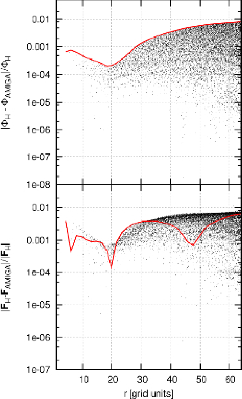
As a first (static) test for the numerical potential solver, we present the recovery of the analytical potential for a known analytical solution of the MONDian Poisson’s equation (4). To this extent we actually start with an analytical description for a spherically symmetric potential akin to the Hernquist profile (Hernquist, 1990)
| (14) |
We added a logarithm to the potential in order to mach the properties of the solution of the MOND equation (far from any source, the MONDian forces are proportional to ). We then derive the density by substituting Eq. (14) into Eq. (4)
| (15) |
The test is performed with non-periodic boundary conditions on a regular 643 grid by fixing the solution on the border to the analytical values. Figure 3 now shows the fractional error in the potential (upper panel) and force (lower panel). The constants in the potential for this particular test are: , Mpc and Mpc. The box used was Mpc. With this choice for the parameters, the force gradually changes from a purely Newtonian regime in the central parts to deep MONDian in the outer regions. The fractional errors are calculated as the difference between the analytical potential and forces on the grid and the numerical solution obtained by our solver. The solid red line shows the error as a function of radius along the diagonal in the box while the dots represent a random sample of all grid points.11 1 Note that running along the 3-dimensional diagonal will coincide with the largest possible error and hence the solid line in the upper panel of Figure 3 marks the upper boundary of the error in the potential. We can clearly see that the error is never larger than 1 per cent indicating the excellent quality of our numerical integration scheme.
3.2.2 Dynamic test


Having established the credibility of our numerical integrator for Eq. (4), we now test the temporal evolution of our code by using a cosmological simulation in the Newtonian limit, i.e. lowering the MONDian acceleration to such a low value that it will not impact upon structure formation. For that purpose we used cm/s2 and compare the final output to a simulation run with the standard Newtonian -body code. The simulation fascilitated particles in a box of comoving side length . The cosmology is characterized by =0.3, =0.7, =0.9, and but actually of no relevance for this particular test.
A first visual impression of the density field in given in Figure 4 where we show the grey-scaled density at each particle position of the simulation at redshift . The differences are at best marginal indicating that the modified solver performs correctly in the Newtonian limit. A more quantitative comparison can be found in Figure 5 where we show the matter power spectrum at redshift . The curves are indistinguishable which is proven by the ratio of the two curves plotted as a dotted line (lowered for clarity by the factor 0.001). We further ran the MPI enabled halo finder AHF22 2 AHF is the successor of MHF introduced in Gill et al. (2004). (Knollmann et al. 2008, in prep.) over both simulations. The resulting mass functions of identified objects is given in Figure 6. Again, there are at best differences that are readily ascribed to numerical errors during the time integration due to our vastly different schemes of solving Poisson’s equation in the two test runs.
4 Cosmological simulations
To date there is only a limited number of cosmological simulations aiming at studying the effect sof MOND in a full cosmological context (Nusser, 2002, KG04). However, both these investigations “simply” solved for the Newtonian forces and modified them according to a non-cosmological MOND prescription prior to being used with the equations-of-motion (cf. Eq. (1)). They both showed that, under their respective heuristic formulations, MOND can lead to large-scale clustering patterns aking to a CDM model.
In the present study we are going to abandon (at least) one of the assumptions made by these authors, namely that and hence that Eq. (6) can be inverted to obtain a function . Here we numerically integrate the MONDian analogue to Poisson’s equation (4) which directly leads to considering the influence of the yet unkown and unregarded curl-field in the process of structure formation. The “only” assumption we adhere to is that MOND does not affects fluctuations and leaves the background cosmology intact (Nusser, 2002; Knebe et al., 2004, e.g.,). We defer to a later study that will make use of modified Friedmann equations accounting for the effects of MOND.
4.1 The Simulation Details
| label | [cm/s2] | |||||
|---|---|---|---|---|---|---|
| CDM | 0.30 | 0.04 | 0.7 | 0.88 | 0.88 | — |
| OCBMond | 0.04 | 0.04 | 0.0 | 0.92 | 0.40 | 1.2 |
| OCBMond2 | 0.04 | 0.04 | 0.0 | 0.92 | 0.40 | 1.2 |
Following KG04 and using the input power spectra derived with the CMBFAST code (Seljak & Zaldarriaga, 1996) we displace particles from their initial positions on a regular lattice using the Zel’dovich approximation (Efstathiou et al., 1985). The box size was chosen to be 32 on a side. This choice guarantees proper treatment of the fundamental mode which will still be in the linear regime at (cf. the scale turning non-linear at is roughly 20 for the models under investigation). The particulars (and terminology) of the models under investigation are summarized in Table 1.
As we used the (Newtonian) Zeldovich approximation to generate the initial conditions we need to make sure that the universe is still Newtonian at the starting redshift. To this extent our choice for the (free) function in Eq. (4) is . This ensures that and hence Eq. (4) reduces to the Newtonian case Eq. (2). We need to acknowledge that this differs from the treatment in KG04 who actually used ; their simulations did not start early enough and were in parts already MONDian at the initial redshift. However, as we will see later on during the analysis of the runs that our results hardly differ from the findings of KG04. We further like to mention that the present study does not aim at distinguishing one MOND theory from another! We merely apply our novel solver to one particular MOND model of our choice showing that this implementation can lead to results that are at least comparable to the favoured CDM structure formation scenario. Besides, we also like to study the effects of the yet unregarded and unkown curl-field upon gravitational structure formation, irrespective of the applicability of our particular MOND model to reality; we leave a detailed study of various MOND realisations to a future paper.
The particles were evolved from redshift until and in all three runs a force resolution of 6 was reached in the highest density regions. The mass resolution of the runs is for the CDM model and for the two low- models, respectively. We output 26 snapshots of the particle positions and velocities equally spaced in time inbetween redshifts and . These outputs are then analysed with respect to their large-scale clustering patterns as well as properties of individual objects employing the MPI enabled halo finder AHF again. For that purpose we though switched off the unbinding procedure; we rather collect all particles within a certain region of a local density peak and refer to them as “object particles” defining the properties of that object. To be more precise, AHF locates density maxima in the simulation by invoking the original adaptive-mesh hierarchy again used during the simulation procedure. For each of these peaks we step out in logarithmically spaced radial bins until the mean density inside that (spherical) sphere drops below a fiducial value where is the cosmological background density, i.e.
| (16) |
defines the edge of an object. However, one needs to carefully choose the correct overdensity which is much higher for the OCBMond models due to the low value. The parameters used are for CDM and for OCBMond (see Gross, 1997, Appendix C, and references therein). 33 3 Note that depends both on redshift and cosmology.
4.2 The Matter Field


We start with inspecting the matter density field of all three runs in Figure 7. There we can see that at redshift the differences amongst the models are rather small. However, there are major differences at larger redhifts due to the fact that the formation of structures under MOND kicks in later and then at an increased growth rate (i.e. in MOND as opposed to for Newtonian physics, e.g. Sanders (2001); Nusser (2002); Knebe et al. (2004); Sanders (2008)). But the more interesting observation is the comparison between our two MONDian implementations. There we can see some objects that are still approaching each other in OCBMond to have already merged in OCBMond2 indicative of an advanced evolutionary stage.
We quantify the evolutionary stage in Figure 8 where we present the matter power spectra at redshift , , and . We basically recover the same features as reported by KG04 (even though they considered a rather different MOND model with ), namely the lack of a distinctive “break” due to the transfer of power from large to small scales in the MONDian runs and the (marginally) larger amplitude of power on scales Mpc-1 close to the fundamental mode. However, we also observe that OCBMond2 evolved marginally faster on large scale and at later times than OCBMond.
A rather natural question arises about the sites where MOND is actually affective. To shed some light on this issue we show in Figure 9 the modulus of the MONDian force in the OCBMond2 model at the particle positions at redshift normalized by (which corresponds to the argument of the MONDian interpolation function used with Eq. (4)). We find that particles in low-density regions and the vicinity of objects, respectively, are in the MOND regime whereas particles residing at the centres of objects (i.e. high-density regions) are mostly unaffected by MOND. This may result in different (hierarchical?) structure formation scenarios as matter infall onto objects will most certainly be affected by the “MONDian environment” of objects. We will investigate this in the following Section.
4.3 Hierarchical Structure Formation


As already noted in Figure 7 and 8 there appears to be a marginally faster evolution of (large-scale) structures in OCBMond2. This is further confirmed in Figure 10 where we show the abundance evolution of objects with mass . At around redshift OCBMond2 starts to develop more objects. Anyways, the late onset and faster evolution of structure formation under MOND in general was already reported by Sanders (2001), Nusser (2002) and KG04. However, here we not only used a differnet MOND model but also revised the way of presenting the comparison between the two MONDian and the Newtonian runs. As OCBMond and OCBMond2 are simulations of the gravitational interactions of baryons whereas the CDM model contains both baryonic and dark matter a fair comparision should correct for that. Or in other words, an object of mass in one of the MOND runs merely contains baryons whereas the corresponding object in CDM contains both baryons and dark matter. As the idea of MOND is to replace dark matter by a modification to Newtonian dynamics we should “remove” the dark halo from the CDM object when performing a cross-comparison. We therefore multiply the CDM masses by the cosmic baryon fraction and refer to all masses as “baryonic mass” even though the interactions of baryons other than gravity are not modelled in the simulations presented in this study. We note that this is not necessarily correct as galaxies probably contain fewer baryons than given by the cosmic baryon fraction (Gottlöber & Yepes, 2007; Okamoto et al., 2008, e.g., ). Our “baryonic” CDM masses are therefore considered an upper limit and are likely to be smaller.
By revising the mass of CDM dark matter halos we note that the abundance evolution is similar yet different when comparing CDM against the two MONDian models. Similar in a sense that the in KG04 advocated dramatic difference at high redshift is not as pronounced anymore. However, the actual shape of the Newtonian and MONDian curves are though rather different with a more gentle increase in the number of objects in CDM (at least at redshifts smaller than ).
To gain a better understanding of structure formation under MOND we constructed a merger tree for each individual object identified at redshift . We then fitted the universal mass accretion history formula to the data (Wechsler et al., 2002)
| (17) |
Applying the half-mass criterion (Tormen, 1997, e.g.,) to the fits for obtaining the formation redshift (i.e. the formation redshift is implicitly defined via )44 4 Even though we stored 26 snapshots between redshifts and for each model we prefer to use the fitted mass accretion history as it will provide us with a more precise estimate for the formation time. we are able to quantify hierarchical structure formation. We expect small objects to form first and then successively merge to form larger and larger entities (Davis et al., 1985, e.g.,). This can be verfied in Figure 11 where we plot today’s mass against the formation redshift of that object. We note a clear hierarchical tendency even in both MOND models. To quantify differences we fitted a simple power law to the data
| (18) |
where the best fit is given in the upper right corner of the respective panel. We find that especially in OCBMond2 high-mass objects appear to form at earlier times than in CDM. Note that this does not contradict the dearth of massive objects at high redshifts as observed in Figure 10. Here we are tracing back individual objects whereas in Figure 10 we considered all objects above a given mass at a certain redshift; Figure 11 simply indicates that (some of) the high mass objects found at redshift must have already been in place at a higher redshift than in, for instance, CDM. Surprisingly there is also a difference between OCBMond and OCBmond2 with the former being closer to CDM. This highlights the relevance of the curl-field introduced in Eq. (6) for structure formation.
One of the findings of the study by KG04 was that the (formation) sites of MONDian objects are marginally more correlated. Can we vindicate that the two-point correlation function of MONDian objects (i.e. galaxies and hence the subscript ) has a larger amplitude (at least) on small scales. This can be verified in Figure 12 where we plot for the 1000 most massive objects in all three models. We confirm the finding of KG04 that OCBMond has a (marginally) larger amplitude than CDM, especially on small scales. We further acknowledge that OCBMond2 has a substantially larger amplitude! In order to better gauge the orgin of the difference between OCBMond and OCBMond2 we split our objects up into different mass bins (i.e. , , ) and calculate for each mass bin independently. The results can be viewed in Figure 13. We observe that the differences are due to the biased formation sites of high-mass objects. We like to mention that the number of objects in each mass bin is practically identical amongst OCBMond and OCBMond2; only in the range there are about 24% more objects in OCBMond2 as indicated by Figure 10. We hence ascribe the bias between OCBMond and OCBMond2 as found in Figure 12 to the large mass objects and hence the stronger evolution of large scales as already seen in Figure 7 and 8.
4.4 Cross-Correlation of Properties


Something not considered in the study of KG04 is the cross-correlation of individual objects. To this extent we use the tool MergerTree that comes with the distribution of the -body code AMIGA and serves the purpose of identifying corresponding objects either in the same simulation at different redshifts (and hence the name “MergerTree”) or in simulations of different cosmological models but run with the same initial phases for the initial conditions. The cross-correlation is done by linking objects that share the most common particles.
We start with the most simple yet still interesting quantify for our cross-comparison, namely the mass . In Figure 14 we show how correlates across CDM and OCBMond (upper panel) as well as across OCBMond and OCBMond2 (lower panel). Remember that we defined as the “baryonic” mass of our halos that coincides with the actual total mass in the two MOND models but corresponds to for CDM; by the usage of the cosmic baryon fraction in this formula we will have an upper limit for the “baryonic” CDM mass (Gottlöber & Yepes, 2007; Okamoto et al., 2008, cf. ). Despite the “baryonic” correction we still observe a difference between the masses of “identical” objects in CDM and the MONDian runs. This can in parts be ascribed to the use of the cosmic baryon fraction and in parts to the definition of the edge of objects: remember that we use for CDM as opposed to for MOND. The latter value translates into a smaller radius and hence less mass. When applying the same density threshold of to the MONDian runs (not presented here though) the MONDian masses increase by approximately 30% bringing them into better (yet not perfect) agreement with the CDM masses.
The other interesting observation in Figure 14 is the fact that there is a systematical difference between the masses of cross-identified objects in OCBMond and OCBMond2. While the most massive objects appear to have identical masses, there is a clear trend for low-mass OCBMond2 objects to be more massive than their OCBMond counterparts. This difference flattens to values closer to unity when considering objects at higher redshift. This phenomenon can therefore be ascribed and explained by the even stronger evolution of the OCBMond2 simulation as already noticed in Figure 7 and Figure 10, respectively. As pointed out by Figure 9, MOND is most affective in the outer regions of objects and hence leaving its imprint via differing infall patterns of material. We therefore ascribed the differences to variation in the mass accretion histories as confirmed by Figure 11.
We close this Section with a brief investigation of the shape of objects as defined by, for instance, the triaxiality parameter (Franx et al., 1991)
| (19) |
where are the principal axes of the moment of intertia tensor we note that there are hardly any differences at all. This can be verified in Figure 15 where we plot for the same set of cross-identified halos as already used in Figure 14 the ratio of the respective triaxialities as a function of mass again. This figure highlights that despite variations in the mass growth of objects at least their triaxialities are unaffected.
4.5 The curl field


As we have just seen there are subtle yet noticable differences when using our novel Poisson solver for the MONDian equation (4) as oppossed to the simplified prescription of inverting Eq. (6) under the assumption of . In that regards it appears mandatory to study the origin of these devations. We therefore present in this Section a detailed investigation of the curl-field and its effects upon structure formation.
| (20) |
Note that setting corresponds to the OCBMond model.
In order to clarify all definitions and terminology to be used from now on we show in Figure 16 a sketch of all the vectors , , and in play. The assumptions used with the OCBMond model imply that the forces there and the Newtonian forces, and , are parallel whereas they both can have an angle with the OCBMond2 force vector . This angle is due to the influence of the curl-field and can be described by the angle (cf. Eq. (20)).
Interpreting the curl-field as a modification to on the right-hand side of Eq. (6) the question arises about the actual adjustment to (the implicitly defined) stemming from this additional ”source” term. We therefore normalize C by the Newtonian acceleration and study its spatial dependence. This can be viewed in Figure 17 where we show (lower panel) in a slice of thickness 125 in the OCBMond2 simulation as calculated on a 2563 grid. We do observe a marginal correlation of the “correction to the source” with the actual matter density shown in the upper panel. We further note that the modulus of the curl-field is actually always smaller than the Newtonian force, however, its spatial variation is though highly non-trivial. In some (high-density) regions there appear to be some kind of “shocks” where the curl-field changes dramatically changes its value. The only conclusion we can draw from this qualitative analysis is that the curl-field has an influence primarily in low-density regions: its value is close to the Newtonian force in the void regions. Finally we like to remark on the “diamond shapes” seen in Figure 17; they are an artifact of the periodic boundary conditions and stem from the periodic images of the largest object/void. These attracting images create the observed symmetry leading to the diamond shapes.
In order to make a more quantitative analysis of the curl-field, we use the snapshots of the simulation OCBMond2 and calculate the Newtonian as well as the two MONDian forces at various redshifts. These forces are then extrapolated to the particle positions in the same way as done during the time integration of Eq. (1). We are aware that this extrapolation will bias our results towards high-density regions (where the particles actually reside) and ignore the effects-of-interest in low-density regions, respectively. However, our integration scheme is based upon the idea of sampling phase-space with particles and hence the forces at the particle positions are relevant for the time integration of Eq. (1) and hence the evolution of the simulation.
In Figure 18 we now present a quantitative comparison of the curl field, , and the Newtonian forces by plotting the probability distribution of the angle between the two vectors (upper panel) as well as the relative difference of the modulus (lower panel). First, we note that there is practically no evolution with redshift. Second, the curl-field is well aligned with the Newtonian force though it may also point in the opposite direction! In order to emphasize the skewness of the distribution about we show the modulus of it. The upper curves thereby correspond to , i.e. it is more likely that the curl points in the opposite direction. However, the lower panel of Figure 18 indicates that the actual change to the “source” term for the implicitly defined (cf. Eq. (6)) induced by the curl is rather small. Here we show the fractional difference between the moduli of the curl and the Newtonian force vector. This distribution peaks at approximately and hence a 10% correction to in Eq. (6); this modification is again independent of redshift. So, the net effect of the curl field is to reduce the “source” on the right hand side of Eq. (6). We expect this to translate into a reduction of with respect to , too.
But because of the implicit definition and the vector-nature of the quantities involved in the calculation of it is difficult to make predictions for the change in induced by the modifications to the “source” in Eq. (6). We therefore plot in Figure 19 the analogous quantities as in Figure 18 this time for the comparison of and ; this should reveal the effects of the curl-field directly. As the angle distribution is no longer symmetric we expand it over the whole range from . The upper panel (showing the angle distribution) clearly indicates that both MONDian forces are well aligned (note the logarithmic scale on the -axis). The lower panel (showing the fractional difference between and ) proofs what we already expected: the distribution is centered about but shows a skewness towards values of stronger and lower , respectively. This skewness is a manifestation of the result obsvered in Figure 18, namely that the curl preferentially decreases the “source” in Eq. (6).
We further note in Figure 19 that there is a marginal redshift evolution of the peak in the distribution of the fractional differences of the two MONDian forces. The peak gradually migrates away from at redshift towards more negative values of approximately at . While it appears counter-intuative to explain the advanced structure formation in OCBMond2 found in previous Sections (cf. Figure 7, Figure 8, Figure 10, etc.) with the finding that the forces are smaller in that model, we rather believe that the shift in the peak can be held responsible for it. This shift towards negative values translates into stronger OCBMond2 forces and hence structure formation at an accelerated speed.
As an illustrative example of the misalignment between the two MONDian forces (and its relation to the underlying density field) we show in Figure 20 both the (colour-coded) cosine of the angle between and (left panel) alongside the density at the particles’ positions at redshift . We note that there is no apparant correlation of the misalignment with density.
5 Summary & Conclusions
We presented a novel solver for the analogue to Poisson’s equation taking into account the effects of modified Newtonian dynamics (MOND). This equation is a highly non-linear partial differential equation for which standard solvers based upon Fourier transformation techniques and/or tree structures are not applicable anymore; one has to defer to multi-grid relaxation techniques (Brandt, 1977; Press et al., 1992; Knebe et al., 2001, e.g.,) in order to numerically solve it.
The major part of this paper hence deals with the necessary (non-trivial) adaptions to the existing multi-grid relaxation solver AMIGA (successor to MLAPM introduced by Knebe et al. (2001)). We show that the accuracy of our MOND solver is at a credible level for a static problem with known MONDian solution and that it reproduces correct results in the Newtonian limit for cosmological simulations.
In the case that we don’t want to adhere to any (undjustifyable and hence ad-hoc) assumptions as, for instance, done by KG04, we are facing the problem that there is still a lot of freedom from the covariant point of view to describe the original phenomenological MOND theory. To be able to actually perform MONDian cosmological simulations we decided to choose one particular model for MOND and to leave for later studies the analysis of the effects that differents theories producces on the structure formation. One of the suppositions KG04 made relates to the relation between the MONDian and the Newtonian force vector. They use the rather simple relation as given by setting in Eq. (6) making the right-hand side simply the Newtonian force. This implicit definition for could be inverted and used instead of when updating the particles’ velocities during the time integration of Eq. (1). As noted in Eq. (6) they neglected the so-called MONDian curl-field . Others have shown that this field decreases like and vanishes for any kind of symmetry (Bekenstein & Milgrom, 1984), it yet remains unclear whether it will leave any imprint on inhomogeneous strucure formation as found in cosmological simulations.
In the second part of this paper we therefore presented a series of cosmological simulations set out to quantify both structure formation under MOND as well as the effects of the curl-field. Surprisingly, we found that our results are consistent with KG04 even if we take in account that they use a different MOND model and initial conditions generated with standard linear theory in a MONDian regimen. We revised some of their findings (mainly the discrepancy between the abundance of galaxies at galaxies at high redshift between CDM and OCBMond) and noted that the curl-field leaves marginal yet noticable effects. The major result of this study though is that the curl-field appears to drive structure formation! Our results obtained with the new solver (and hence including the effects of the curl-field) can be summarized as follows
- •
the curl-field drives structure formation,
- •
the curl-field leads to more objects at where
- •
cross-identified objects are more massive in OCBMond2 than in OCBMond, and
- •
the OCBMond2 model shows a stronger two-point correlation function.
We acknowledge that there are still a lot of puzzling results to be investigated in greater detail. However, we postpone this to future studies. The aim of this paper was primarily to describe the novel gravity solver that is freely available for download.55 5 AMIGA can be downloaded from the following web page http://www.aip.de/People/aknebe/AMIGA. The new MOND solver can be switched on via the compilation flag -DMOND2. The code is able to run cosmological simulations, ie with expansion and periodic boundary conditions and to work also in isolation, wich implies no expansion and fixed boundary conditions. It can be also use without temporal evolution in order to get 3D potentials from density distributions given by particles or analitic formulas. Please contact the authors for more details.
Acknowledgements
CLL and AK acknowledge funding by the DFG under grant KN 755/2. AK further acknowledges funding through the Emmy Noether programme of the DFG (KN 755/1). CLL is gratefull to Xufen Wu for her support during the testing phase of the code. The simulations and analysis were carried out on the AIP’s supercomputing cluster.
References
- Bekenstein & Milgrom (1984) Bekenstein J., Milgrom M., 1984, ApJ, 286, 7
- Bekenstein (2004) Bekenstein J. D., 2004, Phys. Rev. D, 70, 083509
- Binney & Tremaine (1987) Binney J., Tremaine S., 1987, Galactic dynamics. Princeton, NJ, Princeton University Press, 1987, 747 p.
- Brada & Milgrom (1999) Brada R., Milgrom M., 1999, ApJ, 519, 590
- Brandt (1977) Brandt A., 1977, Math. of Comp., 31, 333
- Davis et al. (1985) Davis M., Efstathiou G., Frenk C. S., White S. D. M., 1985, ApJ, 292, 371
- de Blok et al. (2003) de Blok W. J. G., Bosma A., McGaugh S., 2003, MNRAS, 340, 657
- Efstathiou et al. (1985) Efstathiou G., Davis M., White S. D. M., Frenk C. S., 1985, ApJS, 57, 241
- Franx et al. (1991) Franx M., Illingworth G., de Zeeuw T., 1991, ApJ, 383, 112
- Gill et al. (2004) Gill S. P. D., Knebe A., Gibson B. K., 2004, MNRAS, 351, 399
- Gottlöber & Yepes (2007) Gottlöber S., Yepes G., 2007, ApJ, 664, 117
- Gross (1997) Gross M. A. K., 1997, PhD thesis, AA(UNIVERSITY OF CALIFORNIA, SANTA CRUZ)
- Halle et al. (2007) Halle A., Zhao H., Li B., 2007, ArXiv e-prints, 711
- Hernquist (1990) Hernquist L., 1990, ApJ, 356, 359
- Klypin et al. (1999) Klypin A., Gottlöber S., Kravtsov A. V., Khokhlov A. M., 1999, ApJ, 516, 530
- Knebe et al. (2004) Knebe A., Gill S. P. D., Gibson B. K., Lewis G. F., Ibata R. A., Dopita M. A., 2004, ApJ, 603, 7
- Knebe et al. (2001) Knebe A., Green A., Binney J., 2001, MNRAS, 325, 845
- Komatsu et al. (2008) Komatsu E., Dunkley J., Nolta M. R., Bennett C. L., Gold B., Hinshaw G., Jarosik N., Larson D., Limon M., Page L., Spergel D. N., Halpern M., Hill R. S., Kogut A., Meyer S. S., Tucker G. S., Weiland J. L., Wollack E., Wright E. L., 2008, ArXiv e-prints, 803
- Milgrom (1983) Milgrom M., 1983, ApJ, 270, 365
- Moore et al. (1999) Moore B., Ghigna S., Governato F., Lake G., Quinn T., Stadel J., Tozzi P., 1999, ApJ, 524, L19
- Nipoti et al. (2007) Nipoti C., Londrillo P., Ciotti L., 2007, ApJ, 660, 256
- Nusser (2002) Nusser A., 2002, MNRAS, 331, 909
- Okamoto et al. (2008) Okamoto T., Gao L., Theuns T., 2008, ArXiv e-prints, 806
- Press et al. (1992) Press W. H., Teukolsky S. A., Vetterling W. T., Flannery B. P., 1992, Numerical recipes in C. The art of scientific computing. Cambridge: University Press, —c1992, 2nd ed.
- Sanders (2001) Sanders R. H., 2001, ApJ, 560, 1
- Sanders (2008) Sanders R. H., 2008, MNRAS, pp 463–+
- Seljak & Zaldarriaga (1996) Seljak U., Zaldarriaga M., 1996, ApJ, 469, 437
- Skordis (2008) Skordis C., 2008, Phys. Rev. D, 77, 123502
- Swaters et al. (2003) Swaters R. A., Madore B. F., van den Bosch F. C., Balcells M., 2003, ApJ, 583, 732
- Tiret & Combes (2007) Tiret O., Combes F., 2007, A&A, 464, 517
- Tormen (1997) Tormen G., 1997, MNRAS, 290, 411
- Wechsler et al. (2002) Wechsler R. H., Bullock J. S., Primack J. R., Kravtsov A. V., Dekel A., 2002, ApJ, 568, 52
- Wesseling (1992) Wesseling P., 1992, An Introduction to Multigrid Methods. John Wiley and Sons Inc, —c1992, 2nd ed.
- Zhao (2007) Zhao H., 2007, ApJ, 671, L1
- Zhao (2008) Zhao H., 2008, ArXiv e-prints, 805