Precise $\alpha_{\scriptscriptstyle S}$ from $\tau$ Decays

The hadronic decays of the $\tau$ lepton provide a clean laboratory to perform precise studies of QCD. Invariant mass distributions obtained from long distance hadron data allow one to compute the spectral functions, which permit the study of short distance quark interactions. In particular, these spectral functions can be exploited to precisely determine the strong coupling constant at the $\tau$-mass scale, $\alpha_{\scriptscriptstyle S}(m_{\tau}^{2})$ . Most of the present analysis is described in detail in ref [1]. Some new studies on the perturbative methods are described in Sec. 3.

The nonstrange vector (axial-vector) spectral functions $v_{1}(a_{1})$, for a spin 1 hadronic system, are obtained from the squared hadronic mass distribution, normalised to the hadronic branching fraction (with the hadronic observable(s) $R_{\tau,V/A}=\frac{\cal{B}_{\tau\to V^{-}/A^{-}(\gamma)\nu_{\tau}}}{\cal{B}_{\tau\to{\text{e}}^{-}\overline{\nu}_{\text{e}}\nu_{\tau}}}$), and divided by a factor exhibiting kinematics and spin characteristics

The basis for comparing a theoretical description of strong interaction with hadronic data is provided by the optical theorem, which relates the imaginary part of the polarisation functions on the branch cut along the real axis, to the spectral functions: $2\pi\cdot Im\Pi^{1}_{V/A}(s)=v_{1}/a_{1}(s)$.

The determinations of $R_{\tau}$ from measured leptonic branching ratios, or only from the electronic one assuming universality, are in very good agreement, yielding $R_{\tau}=({1-\cal{B}_{\text{e}}-\cal{B}_{\mu}})/{\cal{B}_{\text{e}}}={1}/{\cal{B}_{\text{e}}^{\rm uni}}-1.9726=3.640\pm 0.010\>.$ One can identify in $R_{\tau}$ a component with net strangeness and two nonstrange vector(V) and axial-vector(A) components. Including the latest results from BABAR and Belle the value of the strange component is $R_{\tau,S}=0.1615\pm 0.0040\>.$ The separation of the V and A components for final states with only pions is done using G-parity. For the $K\kern 1.99997pt\overline{\kern-1.99997ptK}{}\pi$ mode, we assume CVC and use new results from the BABAR Collaboration [2]. Finally, we get the components: $R_{\tau,V}=1.783\pm 0.011\pm 0.002$ and $R_{\tau,A}=1.695\pm 0.011\pm 0.002\>,$ where the first errors are experimental and the second due to the $V/A$ separation.

The nonstrange ratio $R_{\tau,V/A}$ can be written as an integral of the spectral functions over the invariant mass-squared $s$ of the final state hadrons

The two point correlator can not be predicted by QCD in this region of the real axis. However, using Cauchy’s theorem, one can relate this expression to an integral on a circle in the complex plane. Then, the OPE yields $R_{\tau,V/A}\propto 1+\delta^{(0)}+\delta^{\prime}_{\rm EW}+\delta^{(2,m_{q})}_{ud,V/A}+\sum_{D=4,6,\dots}\delta_{ud,V/A}^{(D)}\>,$ with a massless perturbative contribution, a non-logarithmic electroweak correction, the dimension two perturbative quark-mass contribution and higher dimension nonperturbative condensates contributions respectively. The perturbative part reads $\delta^{(0)}=\sum_{n=1}^{\infty}\tilde{K}_{n}(\xi)A^{(n)}(\alpha_{\scriptscriptstyle S})\>,$ with the functions

where $a_{s}\hskip-2.84544pt\equiv\hskip-2.84544pt{\alpha_{s}}/{\pi}$ and $\xi$ is a scale factor. A breakthrough was made recently [3], so that the pertubative coefficients are now known up to $\tilde{K}_{4}$ (see [1] for the numerical values of the $\tilde{K}_{n}(\xi)$ coefficients).

In order to obtain additional experimental information, we use spectral moments defined as

They allow one to better exploit the shape of the spectral functions and they suppress the region where OPE fails. The corresponding theoretical prediction is very similar to the one for $R_{\tau}\>,$ with consequent perturbative and nonperturbative contributions. Due to strong correlations, we use only $R_{\tau}$ ($k=0$ and $l=0$) and four additional moments ($k=1$ and $l=0,1,2,3$) to simultaneously fit $\alpha_{\scriptscriptstyle S}(m_{\tau}^{2})$ and the leading D = 4, 6, 8 nonperturbative contributions.

In spite of the fact that the nonperturbative contributions fitted for the V and A spectral functions have opposite signs and they are much larger than those from V+A, we find an excellent agreement between the values found for $\alpha_{\scriptscriptstyle S}(m_{\tau}^{2})$ from the three fits. The result of the fit to the V+A spectral moments reads

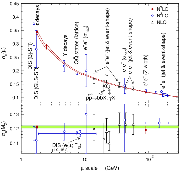
where the first error is experimental and the second is theoretical. When evolving this value to the Z scale [1](see Fig. 2) one gets

where the first two errors are propagated from (9), and the last one summarises uncertainties in the evolution. The consistency between this result and the value found by a global fit to electroweak data at the Z-mass scale [1], $\alpha_{\scriptscriptstyle S}^{(\tau)}(m_{Z}^{2})-\alpha_{\scriptscriptstyle S}^{(Z)}(m_{Z}^{2})=0.0021\pm 0.0029$, provides the most powerful present test of the evolution of the strong interaction coupling, over a range of $s$ spanning more than three orders of magnitude.

Motivated by some new results both on theoretical and experimental grounds, we have revisited the determination of $\alpha_{\scriptscriptstyle S}(m_{\tau}^{2})$ from the ALEPH $\tau$ spectral functions. We have re-examined two common numerical methods: we have identified specific consistency problems of FOPT, which do not exist in CIPT. The $\tau$ measurement of $\alpha_{s}$ evolved to the Z scale is found to be in excellent agreement with the direct determination from Z decays. Both results are the only ones at $N^{3}LO$ order so far, confirming the running of $\alpha_{\scriptscriptstyle S}$ between 1.8 and 91 GeV, as predicted by QCD, with an unprecedented precision of $2.4\%$.

References

- [1] M. Davier, S. Descotes-Genon, A. Hocker, B. Malaescu and Z. Zhang, Eur. Phys. J. C 56, 305 (2008) [arXiv:0803.0979 [hep-ph]].
- [2] B. Aubert et al. [BaBar Collaboration], Phys. Rev. D 77, 092002 (2008) [arXiv:0710.4451 [hep-ex]].
- [3] P. A. Baikov, K. G. Chetyrkin and J. H. Kuhn, Phys. Rev. Lett. 101, 012002 (2008) [arXiv:0801.1821 [hep-ph]].
- [4] W. M. Yao et al. [Particle Data Group], J. Phys. G 33 (2006) 1.
- [5] M. Beneke and M. Jamin, arXiv:0806.3156 [hep-ph].