Tensor-product representations for string-net condensed states
Abstract
We show that general string-net condensed states have a natural representation in terms of tensor product states (TPS) . These TPS’s are built from local tensors. They can describe both states with short-range entanglement (such as the symmetry breaking states) and states with long-range entanglement (such as string-net condensed states with topological/quantum order). The tensor product representation provides a kind of ’mean-field’ description for topologically ordered states and could be a powerful way to study quantum phase transitions between such states. As an attempt in this direction, we show that the constructed TPS’s are fixed-points under a certain wave-function renormalization group transformation for quantum states.
I Introduction
In modern condensed matter theory, an essential problem is the classification of phases of matter and the associated phase transitions. Long range correlation and broken symmetry[1] provide the conceptual foundation to the traditional theory of phases. The mathematical description of such a theory is realized very naturally in terms of order parameters and group theory. The Landau symmetry breaking theory was so successful that people started to believe that the symmetry breaking theory described all phases and phase transitions. From this point of view, the discovery of the fractional quantum Hall (FQH) effect[2] in the 1980’s appears even more astonishing than what we realized. These unique phases of matter have taught us a very important lesson, when quantum effects dominate, entirely new kinds of order, orders not associated with any symmetry, are possible.[3] Similarly, new type of quantum phase transitions, such as the continuous phase transitions between states with the same symmetry[4, 5, 6, 7] and incompatible symmetries[8, 9] are possible. There is literally a whole new world of quantum phases and phase transitions waiting to be explored. The conventional approaches, such as symmetry breaking and order parameters, simply does not apply here.
The particular kind of order present in the fractional quantum Hall effect is known as topological order,[3] or more specifically, chiral topological order because of broken parity and time reversal (PT) symmetry. Topological phases which preserve parity and time reversal symmetry are also possible,[10, 11, 12, 13, 14, 15, 16, 7, 17, 18, 19] and we will focus on these phases in this paper. An appealing physical picture has recently been proposed for this large class of PT symmetric topological phases in which the relevant degrees of freedom are string like objects called string-nets.[20, 21] Just as particle condensation provides a physical picture for many symmetry breaking phases, the physics of highly fluctuation strings, string-net condensation, has been found to underlie PT symmetric topological phases.
The physical picture of string-net condensation provides also a natural mathematical framework, tensor category theory, which can be used to write down fixed point wave functions and calculate topological quantum numbers.[21, 22] These topological quantum numbers include the ground state degeneracy on a torus, the statistics and braiding properties of quasi-particles, and topological entanglement entropy.[23, 24] All these physical properties are quite non-local, but they can be studied in a unified and elegant manner using the nonlocal string-net basis.
Unfortunately, this stringy picture for the physics underlying the topological phase seems poorly suited for describing phase transitions out of the topological phase. The large and non-local string-net basis is difficult to deal with in the low energy continuum limit appropriate to a phase transition. Trouble arises from our inability to do mean field theory, to capture the stringiness of the state in an average local way. Indeed, the usual toolbox built around having local order parameters is no longer available since there is no broken symmetry. We are thus naturally led to look for a local description of topological phases which lack traditional order parameters.
Remarkably, there is already a promising candidate for such a local description. A new local ansatz, tensor product states (also called projected entangled pair states), has recently been proposed for a large class of quantum states in dimensions greater than one [25]. In the tensor product state (TPS) construction and its generalizations,[26, 27] the wave function is represented by a local network of tensors giving an efficient description of the state in terms of a small number of variables.
The TPS construction naturally generalizes the matrix product states in one dimension.[28, 29] The matrix product state formulation underlies the tremendous success of the density matrix renormalization group for one dimensional systems.[30] The TPS construction is useful for us because it allows one to locally represent the patterns of long-range quantum entanglement[31, 23, 24] that lies at the heart of topological order. In this paper, we show that the general string-net condensed states constructed in have natural TPS representations. Thus the long-range quantum entanglement in a general (non-chiral) topologically ordered state can be captured by TPS. The local tensors that characterize the topological order can be viewed as the analogue of the local order parameter describing symmetry breaking order.
In addition to our basic construction, we demonstrate a set of invariance properties possessed by the TPS representation of string-net states. These invariance properties are characteristic of fixed point states in a new renormalization group for quantum states called the tensor entanglement renormalization group.[35] This fixed point property of string-net states has already been anticipated[21], and provides a concrete demonstration of string-net states as the infrared limit of PT symmetric topological phases.
This paper is organized as follows. In sections II-III we construct TPS representations for the two simplest string-net condensed states. In section IV we present the general construction. In the last section, we use the TPS representation to show that the string-net condensed states are fixed points of the tensor entanglement renormalization group. Most of the mathematical details can be found in the appendix.

II gauge model
We first explain our construction in the case of the simplest string-net model: lattice gauge theory (also known as the toric code). [18, 17, 20, 21] In this model, the physical degrees of freedom are spin- moments living on the links of a square lattice. The Hamiltonian is
Here is the product of the four around a square and is a sum over all the squares. The term is the product of the four around a vertex and is a sum over all the vertices. The ground state of is known exactly. To understand this state in the string language, we interpret the and states on a single link as the presence or absence of a string. (This string is literally an electric flux line in the gauge theory.) The ground state is simply an equal superposition of all closed string states (e.g. states with an even number of strings incident at each vertex):
| (1) |
While this state is relatively simple, it contains nontrivial topological order. That is, it contains quasiparticle excitations with nontrivial statistics (in this case, Fermi statistics and mutual semion statistics) and it exhibits long range entanglement (as indicated by the non-zero topological entanglement entropy [23, 24]).
The above state has been studied before using TPS [32, 33]. Our TPS construction is different from earlier studies because it is derived naturally from the string-net picture. As illustrated in Fig. 1, we introduce two sets of tensors: -tensors living on the vertices and -tensors living on the links. The -tensors are rank three tensors with one physical index running over the two possible spin states , and two “internal” indices running over some range . The -tensors are rank four tensors with four internal indices running over .
In the TPS construction, we construct a quantum wave function for the spin system from the two tensors ,. The wave function is defined by
| (2) |
To define the tensor-trace (tTr), one can introduce a graphic representation of the tensors (see Fig. 1). Then tTr means summing over all unphysical indices on the connected links of tensor-network.
It is easy to check that the string-net condensed ground state that we discussed above is given by the following choice of tensors with internal indices running over :
| (6) |
The interpretation of these tensors is straightforward. The rank-3 tensor behaves like a projector which essentially sets the internal index equal to the physical index so that represents a string and represents no string. The meaning of the tensor is also clear: it just enforces the closed string constraint, only allowing an even number of strings to meet at a vertex.
In this example, we have shown how to represent the simplest string-net condensed state using the TPS construction. We now explain how to extend this construction to the general case.
III Double-semion model
Let us start by turning to a slightly less straightforward model which illustrates some details necessary for our TPS construction for general string-net states. The model, which we call the double-semion model, is a spin-1/2 model where the spins are located on the links of the honeycomb lattice. The Hamiltonian is defined in Eq. (40) in Ref. 21. Here we will focus on the ground state which is known exactly. As in the previous example, the ground state can be described in the string language by interpreting the and states on a single link as the presence or absence of a string. The ground state wave function is a superposition of closed string states weighted by different phase factors:
| (7) |
where is the number of closed loops in the closed-string state . [20, 21] As in the previous example, this state contains non-trivial topological order. In this case, the state contains quasiparticle excitations with semion statistics.

Like the state, the above string-net condensed state can be written as a TPS with one set of tensors on the vertices and another set of tensors on links. However, in this case it is more natural to use a rank-6 tensor and a rank-5 tensor . These tensors can be represented by double lines as in Fig. 2. The -tensors are given by
| (8) |
where now each internal unphysical index runs over . Here, the tensor is given by
The rank-5 tensors are given by
| (13) |
Again, the ground state wave function can be obtained by summing over all the internal indices on the connected links in the tensor network (see Fig. 2):
| (14) |
From Eq.(13) we see that the physical indices and the internal indices have a simple relation: each pair of internal unphysical indices describes the presence/absence of string on the corresponding link. Two identical indices (00 and 11) in a pair correspond to no string (spin up) on the link and two opposite indices (01 and 10) in a pair correspond to a string (spin down) on the link. We may think of each half of the double line as belonging to an associated hexagon, and because every line along the edge of a hexagon takes the same value, we can assign that value to the hexagon. In this way we may view physical strings as domain walls in some fictitious Ising model as indicated by the coloring in Fig. 2. The peculiar assignment of phases in serve to guarantee the right sign oscillations essentially by counting the number of left and right turns made by the domain wall.
Equation (14) is interesting since the wave function (7) appears to be intrinsically non-local. We cannot determine the number of closed loops by examining a part of a string-net. We have to examine how strings are connected in the whole graph. But such a “non-local” wave function can indeed be expressed as a TPS in terms of local tensors.
IV General string-net models
We now show that the general string-net condensed states constructed in can be written naturally as TPS. To this end, we quickly review the basic properties of the general string-net models and string-net condensed states.
The general string-net models are spin models where the spins live on the links of the honeycomb lattice. Each spin can be in states labeled by . The Hamiltonians for these models are exactly soluble and are defined in Eq. (11) in Ref. 21. Here, we focus on the (string-net condensed) ground states of these Hamiltonians.
In discussing these ground states it will be convenient to use the string picture. In this picture, we regard a link with a spin in state as being occupied by a type- string. We think of a link with as being empty. As in the previous examples, the ground states are superpositions of many different string configurations. However, in the more general case, the strings can branch (e.g. three strings can meet at a vertex).
To specify a particular string-net model or equivalently a particular string-net condensed state, one needs to provide certain data. First, one needs to specify an integer - the number of string types. Second, one needs to give a rank-3 tensor taking values , where the indices range over . This tensor describes the branching rules: when , that means that the ground state wave function does not include configurations in which strings , , meet at a point. On the other hand, if then such branchings are allowed. Third, the strings can have an orientation and one needs to specify the string type corresponding to a type- string with the opposite orientation. A string is not oriented if . Finally, one needs to specify a complex rank-6 tensor where . The tensor defines a set of local rules which implicitly define the wave function for the string-net condensed state. We would like to mention that the data cannot be specified arbitrarily. They must satisfy special algebraic relations in order to define a valid string-net condensed state.
The main fact that we will use in our construction of the TPS representation of general string-net condensed states is that the string-net condensed states can be constructed by applying local projectors ( is a plaquette of the honeycomb lattice) to a no-string state .[21] These projectors can be written as
| (15) |
where has the simple physical meaning of adding a loop of type- string around the hexagon . The constants are given by
| (16) |
where , and .
This fact enables us to write the string-net condensed state as
| (17) | |||||
where
| (18) |
Note that when , and the order of the operators in the above is not important.
These states are not orthogonal to each other. In the following, we would like to express these states in terms of the orthonormal basis of different string-net configurations:
| (19) |
Here is a string-net configuration and label the string types (i.e. the physical states) on the corresponding link (see Fig. 3c). We note that label the string types associated with the hexagons (see Fig. 3a). As a result, the string-net condensed state is given by
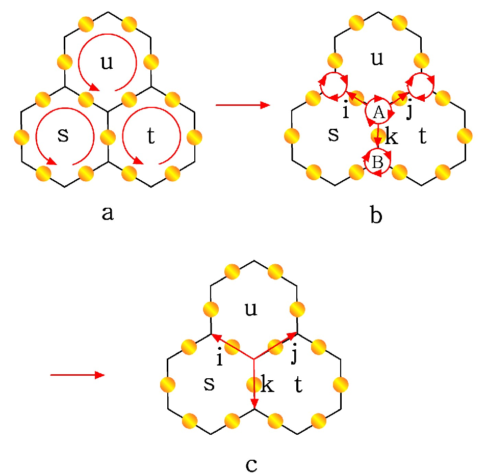

To calculate , we note that the coherent states can be viewed a string-net state in a fattened lattice (see Fig. 3a).[21]. To obtain the string-net states where strings live on the links, we need to combine the two strings looping around two adjacent hexagons into a single string on the link shared by the two hexagons. This can be achieved by using the string-net recoupling rules[21] (see Fig. 3). This allows us to show that the string-net condensed state can be written as (see Appendix A)
| (20) | |||||
where is the symmetric symbol with full tetrahedral symmetry,11 1 Such a is slightly different from that introduced in Ref. 21. and .
Let us explain the above expression in more detail. The indices are on the links while the indices are on the hexagons. Each hexagon contributes to a factor . Each vertex in A-sublattice contributes to a factor and each vertex in B-sublattice contributes to a factor . The indices around a vertex are arranged as illustrated in Fig. 4.


The expression (20) can be formally written as a weighted tensor trace over a tensor-complex formed by -tensors and -tensors. First, let us explain what is a tensor-complex. A tensor-complex is formed by vertices, links, and faces (see Fig. 5). The -tensors live on the vertices and the -tensor live on the links. The -tensor carries the indices from the three connected links and the three adjacent faces, while the tensor carries the indices from the two connected links (see Fig. 6). By having indices on faces, the tensor-complex generalize the tensor-network.
The weighted tensor trace sums over all the indices on the internal links that connect two dots and sums over all the indices on the internal faces that are enclosed by the links, with weighting factors , , etc from each enclosed faces. Let us choose the -tensors on vertices to be (see Fig. 7)
| A-sublattice: | |||||
| B-sublattice: | (21) |
and the tensor to be
| (22) |
In this case the string-net condensed state (20) can be written as a weighted tensor trace over a tensor-complex:
| (23) |
where label the physical states on the links. We note that the -tensor is just a projector: it makes each edge of the hexagon to have the same index that is equal to . The string-net condensed state (20) can also be written as a more standard tensor trace over a tensor-network (see Appendix B).

The string-net states and the corresponding TPS representation can also be generalized to arbitrary trivalent graph in two dimension. After a similar calculation as that on the honeycomb lattice, we find that an expression similar to Eq. (20) describes the string-net condensed state on a generic trivalent graph in two dimension (see Fig. 8a). The indices in Eq. (20), such as , should be read from the Fig. 8a, where the indices of the -symbol is determined by three oriented legs and three faces between them (see Fig. 4).
V The string-net wave function as a fixed point wave function
An interesting property of the string-net condensed states constructed in is that they have a vanishing correlation length: . This suggests that the string-net condensed states are fixed points of some kind of renormalization group transformation. [21] In this section, we attempt to make this proposal concrete. We show that the string-net condensed states are fixed points of the tensor entanglement renormalization group (TERG) introduced in .
To understand and motivate the TERG, it is useful to first think about the problem of computing the norm and local density matrix of the string-net state (24). To obtain the norm, we note that
| (25) | |||||
Thus, the norm can be written as
| (26) | |||||
where we have used the identity .

Here wtTr is a tensor trace over a tensor-complex formed by the double-tensor (see Fig. 9). Again, the tensor-complex are formed by vertices, links and faces. Each trivalent vertex on the A(B)-sublattice represent a double-tensor ():
| (27) |
The double-tensor can be represented by a graph with three oriented legs and three faces between them (see in Fig. 10) where each leg or face now carries two indices. In wtTr, we sum over all indices on the internal links. We also sum over all indices on the internal faces independently with weighting factors from each of the internal faces.
With minor modification, this expression for the norm can be used to compute expectation values for local operators. Indeed, the local density matrix is given by a similar tensor trace, except that the physical indices need to be left unsummed in the region where we want to compute the density matrix. Thus, the problem of computing expectation vales and norms can be reduced to the problem of evaluating the tensor trace (26).
Unfortunately, evaluating tensor traces is an exponentially hard problem in two or higher dimensions. This leads us to the tensor entanglement renormalization group (TERG) method. The idea of the TERG method is to (approximately) evaluate tensor traces by coarse graining. [34] In each coarse graining step, the tensor complex with tensor is reduced to a smaller complex with tensor . Repeating this operation many times allows one to evaluate tensor traces of arbitrarily large complexes. One can therefore compute expectation values of TPS with relatively little effort.
In general, the coarse graining transformation is implemented in an approximate way. That is, one finds a tensor such that . However, as we show below, it can be implemented exactly in the case of the string-net condensed states. Moreover, , so that the string-net condensed states are fixed points of the TERG transformation.
To see this, note that the double--tensor has the following special properties (see Appendix C for a derivation).
Basic rule 1.
The deformation rule of :
| (28) |
Basic rule 2.
The reduction rule of :
| (29) |
The above two basic rules can be represented graphically as in Fig. 11. The two basic rules also lead to another useful property of the double--tensor as represented by Fig. 12.


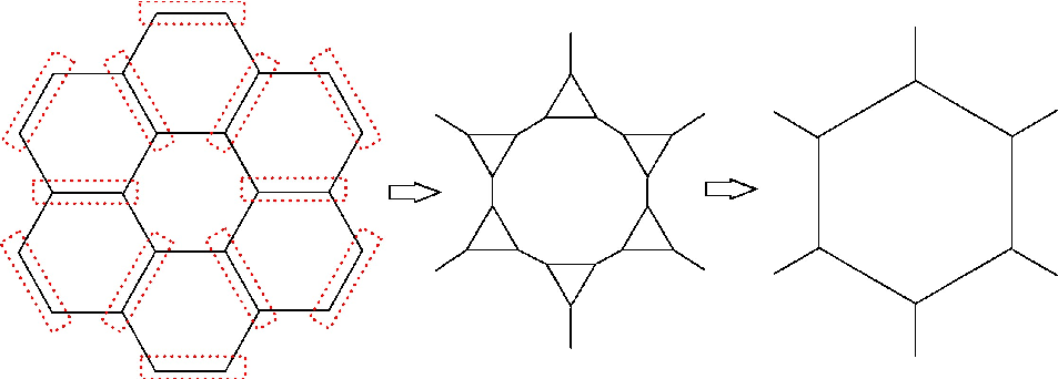
The relations in Fig. 11a and Fig. 12 allow us to reduce the tensor-complex that represents the norm of the string-net condensed state to a coarse-grained tensor-complex of the same shape (see Fig. 13). This coarse-graining transformation is exactly the TERG transformation. Since the tensor is invariant under such a transformation, we see that the string-net wave function is a fixed point of the TERG transformation.
VI Conclusions and discussions
In conclusion, we found a TPS representation for all the string-net condensed states. The local tensors are analogous to local order parameters in Landau’s symmetry broken theory. As a application of TPS representation, we introduced the TERG transformation and show that the TPS obtained from the string-net condensed states are fixed points of the TERG transformation. In Ref. 35, we have shown that all the physical measurements, such average energy of a local Hamiltonian, correlation functions, etc can be calculated very efficiently by using the TERG algorithm under the TPS representations. Thus, TPS representations and TERG algorithm can capture the long range entanglements in topologically ordered states. They may be an effective method and a powerful way to study quantum phases and quantum phase transitions between different topological orders.
We like to mention that a different wave-function renormalization procedure is proposed in . The string-net wave functions are also fixed point wave functions under such a wave-function renormalization procedure.
VII Acknowledgements
This research is supported by the Foundational Questions Institute (FQXi) and NSF Grant DMR-0706078.
Appendix A Tensor product state from string-net recoupling rule
To calculate , we note that the coherent states can be viewed a string-net state in a fattened lattice (see Fig. 3a).[21]. To obtain the string-net states where strings live on the links, we need to combine the two strings looping around two adjacent hexagons into a single string on the link shared by the two hexagons. We make use of the string-net recoupling rules,[21] see Fig. 3, to represent the coherent states in terms of proper orthogonal string states:
where is the string-net state described in Fig. 3b. Note that on each link we have a factor like and we multiply such kind of factors on all links together. Using , we can rewrite the above as
| (30) | |||||
Applying the the string-net recoupling rules again, we rewrite the above as
| (31) | |||||
where is the symmetric symbol with full tetrahedral symmetry. Putting Eq. () into Eq. (17), we finally obtain
| (33) | |||||
We note that the indices, such as , should be read from the Fig. 3. The arrow in(out) on a vertex will determine that we put or in the symbol. In this convention, the physical labels in the symbol are always valued as on sublattice A(arrow in) and on sublattice B(arrow out).
Appendix B String-net condensed state as a TPS on a tensor-network


We have expressed the string-net condensed state (20) as a weighted tensor-trace on the tensor-complex. In this section, we will show that the string-net condensed state (20) can also be written as a more standard tensor-trace over a tensor-network:
| (34) |
Here the tensor-network (see Fig. 14) is formed by two kinds of tensors: a -tensor for each vertex and a -tensor for each link. Unlike the tensors in Fig. 2, now and have a triple-line structure (see Fig. 15). The -tensor on a vertex is given by
| (35) |
where
| (36) |
As shown in in Fig. 4, can be labeled by three oriented lines and three faces between them. Notice that has the cyclic symmetry
due to the tetrahedron symmetry of symbol.
The -tensor on each link is a projector:
| (37) |
where is the physical index running from to and represents the different string types (plus the no-string state). Note that are indices on the side of the A-sublattice and are indices on the side of the B-sublattice. Basically, makes and . The corresponding edge of the hexagon ahs a string of type . The choice of in makes the -tensors to be the same on the A- and B-sublattice.
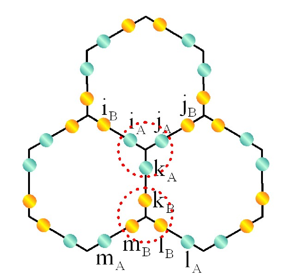
Our construction has a slightly different form from the usual TPS construction, but we can bring our construction into the usual form with a single set of tensors defined on vertices. This is because the matrix on each link is basically a projector (with a twist), so that we can always split it into two matrices and (see Fig. 16) and associate one with each vertex the link touches. Doing this for every link in effect displaces the physical degrees of freedom from the links to the vertices. This procedure seems to enlarge the Hilbert space on each link from to , however, the operators and impose the constraint keeping the physical Hilbert space intact. Grouping the displaced physical degrees of freedom on each vertex into a new physical variable we can combine three sites around each vertex into one site. This is illustrated in Fig. 16, where the states in each dashed circle are labeled by . With this slight reworking of the degrees of freedom, the new tensors on sublattice A and B can be expressed as
with
| (39) |
where are physical indices . Note that the tensors and still have a triple line structure. The string-net condensed state now can be rewritten as
| (40) |
Appendix C Proof of basic rules of
The two basic rules can be proved easily by using the Pentagon Identity[21]. First, the Pentagon Identity leads to a decomposition law for supertensor
| (41) | |||||
Using this expression, it’s easy to proof the two basic rules eqn. (28) and eqn. (29). Here we also use the symmetries of symbol
| (42) |
which can be easily verified from the symmetry of symbol
| (43) |
and the definition of symbol.
Then let us proof the deformation rule eqn. (28).
Proof.
| (44) | |||||
In the last step we use the simple Pentagon Identity[21]
| (45) |
Similarly, we have
| (46) | |||||
finally, we have
| (47) | |||
∎
The reduction rule is also easy to proof by using Pentagon Identity[21].
Proof.
| (48) | |||||
∎
Notice in the third line, we use the fact that .
References
- [1] L. D. Landau, Phys. Z. Sowjetunion 11, 26 (1937).
- [2] D. C. Tsui, H. L. Stormer, and A. C. Gossard, Phys. Rev. Lett. 48, 1559 (1982).
- [3] X.-G. Wen, Int. J. Mod. Phys. B 4, 239 (1990).
- [4] X.-G. Wen and Y.-S. Wu, Phys. Rev. Lett. 70, 1501 (1993).
- [5] T. Senthil, J. B. Marston, and M. P. A. Fisher, Phys. Rev. B 60, 4245 (1999).
- [6] X.-G. Wen, Phys. Rev. Lett. 84, 3950 (2000).
- [7] X.-G. Wen, Phys. Rev. B 65, 165113 (2002a).
- [8] T. Senthil, L. Balents, S. Sachdev, A. Vishwanath, and M. P. A. Fisher, Physical Review B 70, 144407 (2004).
- [9] T. Senthil, Science 303, 1490 (2004).
- [10] N. Read and S. Sachdev, Phys. Rev. Lett. 66, 1773 (1991).
- [11] X.-G. Wen, Phys. Rev. B 44, 2664 (1991).
- [12] T. Senthil and M. P. A. Fisher, Phys. Rev. B 62, 7850 (2000).
- [13] R. Moessner and S. L. Sondhi, Phys. Rev. Lett. 86, 1881 (2001).
- [14] S. Sachdev and K. Park, Annals of Physics (N.Y.) 298, 58 (2002).
- [15] G. Misguich, D. Serban, and V. Pasquier, Phys. Rev. Lett. 89, 137202 (2002).
- [16] L. Balents, M. P. A. Fisher, and S. M. Girvin, Phys. Rev. B 65, 224412 (2002).
- [17] X.-G. Wen, Phys. Rev. Lett. 90, 016803 (2003).
- [18] A. Y. Kitaev, Ann. Phys. (N.Y.) 303, 2 (2003).
- [19] L. B. Ioffe, M. V. Feigel’man, A. Ioselevich, D. Ivanov, M. Troyer, and G. Blatter, Nature 415, 503 (2002).
- [20] M. Freedman, C. Nayak, K. Shtengel, K. Walker, and Z. Wang, Ann. Phys. (NY) 310, 428 (2004).
- [21] M. Levin and X.-G. Wen, Phys. Rev. B 71, 045110 (2005a).
- [22] M. A. Levin and X.-G. Wen, Rev. Mod. Phys. 77, 871 (2005b).
- [23] A. Kitaev and J. Preskill, Phys. Rev. Lett. 96, 110404 (2006).
- [24] M. Levin and X.-G. Wen, Phys. Rev. Lett. 96, 110405 (2006).
- [25] F. Verstraete and J. I. Cirac, cond-mat/0407066.
- [26] G. Vidal, Phys. Rev. Lett. 99, 220405 (2007).
- [27] M. Aguado and G. Vidal, Phys. Rev. Lett. 100, 070404 (2008a).
- [28] A. Klumper, A. Schadschneider, and J. Zittartz, J. Phys. A 24, L955 (1991).
- [29] D. Perez-Garcia, F. Verstraete, M. Wolf, and J. Cirac, Quantum Inf. Comput. 7, 401 (2007).
- [30] S. R. White, Phys. Rev. Lett. 69, 2863 (1992).
- [31] X.-G. Wen, Physics Letters A 300, 175 (2002b).
- [32] F. Verstraete, M. M. Wolf, D. Perez-Garcia, and J. I. Cirac, Phys. Rev. Lett. 96, 220601 (2006).
- [33] M. Aguado and G. Vidal, Phys. Rev. Lett. 100, 070404 (2008b).
- [34] M. Levin and C. P. Nave, Phys. Rev. Lett. 99, 120601 (2007).
- [35] Z.-C. Gu, M. Levin, and X.-G. Wen, arXiv:0806.3509 (2008).