AdS4/CFT3+Gravity for Accelerating Conical Singularities
Mohamed M. Anber11 1 manber@physics.umass.edu
Department of Physics
University of Massachusetts
Amherst, MA 01003
ABSTRACT
We study the quantum-mechanical corrections to two point particles accelerated by a strut in a D flat background. Since the particles are accelerating, we use finite temperature techniques to compute the Green’s function of a conformally coupled scalar applying transparent and Dirichlet boundary conditions at the location of the strut. We find that the induced energy-momentum tensor diverges at the position of the strut unless we impose transparent boundary conditions. Further, we use the regular form of the induced energy-momentum tensor to calculate the gravitational backreaction on the original space. The resulting metric is a constant section of the 4-dimensional C-metric, and it describes two black holes corrected by weakly coupled CFT and accelerating in asymptotically flat spacetime. Interestingly enough, the same form of the metric was obtained before in 0803.2242 by cutting the AdS C-metric with angular dependent critical 2-brane. According to AdS/CFT+gravity conjecture, the latter should describe strongly coupled CFT black holes accelerating on the brane. The presence of the CFT at finite temperature gives us a unique opportunity to study the AdS/CFT+gravity conjecture at finite temperatures. We calculate various thermodynamic parameters to shed light on the nature of the strongly coupled CFT. This is the first use of the duality in a system containing accelerating particles on the brane.
1 Introduction
Since the original construction of the Randall-Sundrum model [1], many authors aimed to find black hole solutions localized on a brane (see e.g. [2]-[15], and [16] for a review). Although this is still an open problem in the case of a 3-brane, Emparan, Horowitz and Myers found a class of brane-localized black holes in the lower dimensional case of a 2-brane embedded in four dimensional Anti-de Sitter space [17, 18]. This was found by appropriately cutting the AdS-C metric [20, 19], which describes bulk accelerated black holes in , with a brane. Since the tension of this brane is determined by its acceleration in the background, this tension is carefully chosen such that the brane acceleration matches the acceleration of the bulk black hole. Recently, this condition was relaxed by detuning the brane tension from the bulk black hole acceleration to find two new classes of solutions on the 2-brane [21]. The first class has time-dependent induced metrics and describes an evolving lump of dark radiation, while the second is a constant -section of the original four-dimensional C-metric and describes accelerated black holes by means of strings or struts.
Moreover, it was conjectured in [22] that black hole solutions localized on a brane in the braneworld correspond to quantum-corrected black holes in dimensions. This conjuncture followed naturally from the AdS/CFT correspondence in which classical dynamics in the bulk encodes the quantum dynamics of the dual D-dimensional conformal field theory (CFT). Thus, solving the classical classical equations in the bulk is equivalent to solving Einstein equations on the brane, where is the D-dimensional Newton’s constant and is the energy-momentum tensor of a strongly coupled CFT with a cutoff in the ultraviolet due to the presence of the brane. This conjecture was put to test in [22] by comparing the brane-black hole solution found in [17] with the one obtained in the dual CFT coupled to gravity. This can be done by starting with a point particle of mass in dimension which generates a deficit angle , and computing the Casimir energy-momentum tensor [23]. Then, one can use this energy-momentum tensor to calculate the backreaction on the conical spacetime [24]. The agreement between the two sides is remarkable and gives a strong argument in favor of the AdS/CFT duality in the context of braneworld scenario. Indeed, this conjecture gives us a convenient way to learn about strong quantum effects in curved backgrounds [25, 26, 27].
According to this conjecture, the accelerated black hole solution found in [21] was interpreted as quantum corrected black hole(s) accelerating on the brane. In the case of a critical brane, this solution describes a pair of black holes accelerated by two strings (or a strut) pulling (pushing) them toward infinity. In the CFT picture, the energy per unit length of this string (strut) has both classical and quantum contributions. Indeed, while in pure dimensional gravity point particles do not interact, quantum effects generate a force between the particles. Hence, the tension of the string (strut) takes into consideration both effects.
In the present work, we calculate the quantum-mechanical backreaction on two point particles attached to a strut and accelerating in D flat background. In our setup, we compute the Green’s function of a conformally coupled scalar. Since we work in an accelerating frame moving with acceleration , it is natural to use a quantum field in equilibrium with a thermal bath at temperature , which is the Hawking-Unruh temperature associated with the Rindler (acceleration) horizon. In calculating the thermal Green’s function, we impose two different boundary conditions at the location of the strut, namely, transparent and Dirichlet boundary conditions. We find that the numerical coefficient of the induced energy-momentum tensor in the first case is identical to the case of a point particle at rest in a D background. On the other hand, the energy-momentum tensor in the case of Dirichlet boundary conditions is divergent at the position of the strut. This suggests that unless we impose transparent boundary conditions, the location of the strut is susceptible to the formation of curvature singularity. Further, we use the resulting energy-momentum tensor calculated in the case of transparent boundary conditions to find the gravitational backreaction on the spacetime. Interestingly enough, we find that the resulting quantum corrected metric has the same form as the one obtained before in [21] by cutting the C-metric with a critical angular dependent brane. Although the former solution describes accelerating black hole dressed with weakly coupled CFT (WCFTBH), the latter, according to AdS/CFT+gravity conjecture, describes accelerating black hole dressed with strongly coupled CFT (SCFTBH). Moreover, the presence of the CFT at finite temperature gives us a unique opportunity to study finite temperature effects in strongly coupled system in curved background. Contrary to the case of the static black hole constructed previusly in [17], where it was found that the black hole mass can be as large as , the largest mass one can place in D, we find that the maximum mass in the present case is temperature dependent. Studying the behavior of this maximum mass reveals a striking difference between the weakly and strongly coupled theories. Although the mass in the former decreases monotonically with temperature from to zero, we find that in the second case it decreases from at low temperatures to a minimum value, and then it increases to again at high temperatures. Further, the black hole horizon circumference diverges in both cases as the mass reaches its maximum value. Beyond this mass, the horizon disappears leaving behind a naked singularity. Actually, it was argued before that quantum effects dresses conical singularities with regular horizon given that these singularities are sufficiently massive. This is known as quantum cosmic censorship [22]. Although this still applies in the case of accelerating conical singularities, supermassive singularities (exceeding the maximum allowed black hole mass at a given temperature) violate this censorship.
We start our treatment using a classical background with a vanishing value of the total mass of particles and strut . After computing the quantum-mechanical backreaction on the spacetime, we find that the mass of the strut gets renormalized which in turn violates the above equality. The violation is minimal for small values of the black hole mass, and becomes stronger for larger values.
Our paper is organized as follows. In section 2 we discuss the background geometry used in the setup. Then, in sections 3 and 4 we calculate the thermal Green’s function and the induced energy-momentum tensor for both transparent and Dirichlet boundary conditions. The gravitational backreaction due to the weakly coupled CFT is computed in section 5, while in section 6 we show that the same form of the metric found in section 5 can be obtained by cutting the AdS C-metric in 4-D with an angular dependent critical brane [21]. The latter describes accelerated black hole dressed with strongly coupled CFT. In section 7 we compute various thermodynamic quantities of the black hole and comment on the AdS/CFT+gravity interpretation of the strongly coupled solution, and finally we conclude in section 8.
2 Background geometry
We start by considering the following metric which describes an accelerating frame moving in a D flat background with acceleration
| (1) |
In order for the metric to have Lorentz signature, we restrict to lie in the range . Also, we restrict to satisfy since the conformal factor implies that the points are infinitely far from those . Moreover, there is a Rindler horizon located at which is a manifestation of the fact that the metric (1) is written in accelerating coordinates. This can be shown using the following set of transformations
| (2) |
which brings (1) to the flat metric . In turn, this restricts to lie in the range , and observers in this system can reach asymptotic infinity at .
Since gravity is not dynamical in D, the presence of a point mass does not alter the geometry in (1). Instead, it affects the global topology of the spacetime. This can be achieved by introducing a deficit parameter and demanding that lies in the new range . The coordinate is, roughly speaking, the inverse radial direction measured from the location of the particle, and hence those values of different from zero reflect the presence of a point mass located at . Since this point mass is accelerating, the acceleration has to be provided by a co-dimensional object, a string or strut 22 2 Although a co-dimensional object is formally a brane, we continue to call it a string (strut) in our setup. Strings correspond to positive tension objects, while struts correspond to negative ones. Strings in D were also studied in [28, 29]. , attached to it. From now on we choose to use a strut located at which extends from the location of the point mass to the Rindler horizon . This choice renders the system well-behaved at asymptotic infinity.


Further, using the toroidal coordinates and , and the Euclidean time , one can write the metric (1) in the form 33 3 The coordinates , and are known in the mathematical physics literature as toroidal or ring coordinates. See e.g. [30, 31].
| (3) |
where and the range maps to . The parameter is defined via where , and corresponds to having empty space. Moreover, we can use the transformations and that bring the metric (3) to the useful form
| (4) |
which is conformal to De Sitter space. In the limit we find , and for empty space lies in the range . Hence, in the presence of the strut we restrict the angle in the range , which can be covered by gluing two copies of the region as sketched in figure(1). The mass of the point particle attached to the strut is determined by reminding that in D the mass is given by . Hence, we find
| (5) |
On the other hand, one can obtain an expression for the energy per unit length, or the force, of the strut. To this end, we write the Israel junction condition for the metric (1)
| (6) |
where and are respectively the jump in the extrinsic curvature and the induced metric at the position of the strut. Hence, we obtain after straight forward calculations noticing the symmetry across the strut
| (7) |
This equation restricts the range of to be . In figure (1b) we see that there are two values of the deficit parameter that correspond to the same tension. We also find that the minimum tension is which occurs at .
The mass of the strut is given by where is the proper length of the strut. The latter can be calculated from (1)
| (8) |
and hence, we obtain
| (9) |
Therefore, we find that the combined mass of the point particle and the strut adds up to zero. We also provide another proof of this result in appendix A by working in the coordinates given in (2). This result is particular to the way we chosed to cut our space and may change upon using more general configurations.
The above construction covers only the half space . The other half describes a particle located at and accelerating in the opposite direction with acceleration horizon located at . This particle is attached to the strut that stretches to the first particle through the horizons.
3 Scalar field quantization
We consider a massless scalar field coupled to a three dimensional background. The corresponding Lagrangian density reads
| (10) |
where is a numerical factor and is the Ricci scalar. The values and correspond to minimally and conformally coupled scalars respectively. Since the Euclidean metric (3) is associated to a background temperature , it is natural to quantize the field incorporating the non-zero temperature techniques. This can be achieved by going to the Euclidean time [32] as we show below.
The Lagrangian (10) leads to the following Euclidean action
| (11) |
where is the Euclidean metric (3). One defines a generating functional through
| (12) |
with being the external current. The thermal average of the time-ordered product of the field operators (the thermal propagator) is given by
| (13) |
where is the Heaviside step function, and the brackets denote the thermal average. Finally, using the generating functional (12) one can show that the propagator satisfies the equation
| (14) |
Now, we are ready to find the normal-mode sum for the propagator in the background (3) 44 4 For scalar field quantization on the BTZ black hole background [33] see [34, 35, 36]. . Since this background is flat, the Ricci scalar vanishes everywhere except at the location of the strut where it is given by with . Moreover, one can show that eq. (14) is separable upon using the ansatz
| (15) |
where we have factored out the conformal factor in (1). Plugging the above ansatz in eq. (14) we obtain in the case of a conformal theory, , a Dirac-delta coefficient that cancels out the contribution from . Hence, in terms of coordinates given in (3) eq.(14) reads
| (16) |
In the following, we consider different boundary conditions that one can impose on the behavior of the two point function at the location of the strut.
Transparent boundary conditions
In this case, we require the propagator to be continuous across the strut, i.e. . Further, by integrating eq. (16) over an interval containing the strut we obtain . This means that the strut is actually transparent to the quantum fluctuations of the conformal theory. Therefore, we find that the normal modes are given by the expansion
| (17) |
where . Substituting the above expansion in eq. (16) we obtain
| (18) |
where . This is associated Legendre equation with well-behaved solution for the range given by
| (19) |
where and , and and are associated Legendre functions of the first and second kind respectively 55 5 For a summary of some properties and relations of associated Legendre functions we use below, see appendix B. [30, 37, 38]. To determine the arbitrary constants , we integrate eq. (18) over an interval containing and use the Wronskian relation (B3) to find . Further, using the addition theorem (B4) we obtain
where .
For the case of empty space, , we can use the identity (B6) to find closed-form expression of the propagator
One can see that is the inverse distance between the space points and given in the Euclideanized version of (2).
The two point function is ultraviolet divergent in the coincidence limit , and one needs to regularize it before proceeding to real calculations. Generally, this can be achieved using Schwinger-DeWitt expansion of the propagator in powers of the geodesic distance between and , and then subtracting the divergent terms which result upon taking the coincidence limit [39]. Fortunately, one does not need this tedious procedure here thanks to the absence of trace anomalies in odd dimensions. Simply, the renormalization can be performed by subtracting out the empty-space contribution . Therefore after using the integral representation of given in (B5), we find
Dirichlet boundary conditions
In this case one requires that the field fluctuations vanish at the position of the strut, i.e. . These boundary conditions are satisfied by the expansion (17) after replacing . Hence, upon going through the same procedure above, we find
where , and .
At this point we are in a position to calculate the renormalized expectation value of the field fluctuations as well as the energy-momentum tensor .
4 Quantum stress tensor
We calculate the expectation value of the field fluctuations as the coincidence limit of the renormalized propagator [39]
| (22) |
which produces upon taking the limit in eq. ()
| (23) |
where is given in appendix C. Interestingly enough, we find that the numerical coefficient in front of the overall factor is identical to the case of a conical singularity with the same mass sitting at rest in D [23]. Similarly, diverges as , the location of the point mass. On the other hand, the above limit in the case of Dirichlet boundary conditions gives
which is divergent at the position of the strut .
The expectation value of the energy-momentum tensor for conformally coupled scalar in flat background is given by [39]
| (25) |
Using the coincidence limit of the various derivatives calculated in appendix C we obtain
| (26) |
where is given in () (see figure (2)). Once more, the numerical factor in front of is equal to that in the case of a conical singularity at rest. This energy-momentum tensor is not of a thermal type although the background used to derive the Green’s function () is in a thermal state. This reflects the presence of a large Casimir component as we have , which violates the strong energy condition.
Taking the coincidence limit (25) for the case of Dirichlet boundary conditions we find
| (27) |
where is given by (C5). The factor is divergent at the location of the strut which is a general property for the energy-momentum tensor with Dirichlet boundary conditions near a curved surface [39, 40]. Since for a conformal energy-momentum tensor one has , we find that this divergent behavior indicates that the location of the strut is susceptible to the formation of a curvature singularity unless we impose transparent boundary conditions.
In the following, we use attempting to find the gravitational backreaction using the semi-classical approximation. We limit our analysis to the case of transparent boundary conditions.


5 Gravitational backreaction
In this section, we use the regularized energy-momentum tensor derived in section 4 in the case of transparent boundary conditions to solve the semi-classical Einstein equations
| (28) |

Since has the form (26), we find that the most general metric that respects this symmetric form is given by
| (29) |
where we have switched back to the Lorentzian time. Substituting the ansatz (29) into (28), it is not difficult to show that the solution is given by
| (30) |
where . Using the coordinates and we finally obtain
| (31) |
This solution is an equatorial section of the four dimensional C-metric [20], and it describes quantum accelerated black holes, with mass given by (5), dressed with weakly coupled CFT in asymptotically flat spacetime.
The function has three zeros , provided that . To have Lorentz signature, the range of is restricted in the range where is the location of the strut. Moreover, has to satisfy , and hence we restrict in the range . Therefore, observers in the accelerating system can reach asymptotic infinity at . As in figure (3), there is a curvature singularity at dressed by a black hole horizon at . Also, there is acceleration horizon at . In section 7, we will see that as one approaches , the position of the strut is pushed closer to the zero , and in the same time the event horizon at closes up with the acceleration horizon at , until the range of disappear when . If , then has only one real zero. In this case, there is a naked curvature singularity to all observers (see [41] for the C-metric in D.) The situation here is completely different from a static point particle sitting in D, where it was found that quantum corrections from a CFT dress the singularity with a regular horizon. This is known as quantum cosmic censorship. The analysis above shows that supermassive accelerating conical singularities in D violate the quantum cosmic censorship. More on this is in section 8.
6 The AdS construction
In this section, we review the construction of the solution (31) using the braneworld scenario [21]. We start with the AdS C-metric in D written in the form [19]
| (32) |
where the functions and are given by
| (33) |
In the above expression we take , and denotes the four dimensional Newton’s constant. This metric describes one or two accelerated black holes with mass and acceleration on Anti-de Sitter (AdS) background with radius . As explained in section 5, the function has three roots provided that . The direction defined by and corresponds to the axis of rotation. To avoid a conical singularity at , we take to have the period . This leaves a conical singularity at which is interpreted in this case as a cosmic string in the bulk that extends from the black hole out to the AdS boundary.

Next, we look for a purely tensional and critical (asymptotically flat) symmetric 2-brane embedded in the above bulk. This brane is described by the surface 66 6 The special case was studied previously in [17]. This corresponds to cutting the bulk with the brane . The brane-induced metric was found to describe a Schwarzschild-like static black hole. . The Israel junction conditions on this surface read
| (34) |
where is the jump in the extrinsic curvature, and is the energy-momentum tensor localized on the brane. For purely tensional and critical brane we have , where is the surface induced metric. Using Israel junction conditions, we find that obeys the differential equation
| (35) |
as well as the auxiliary equation
| (36) |
Although there is no closed-form solution of eq. (35), numerical integration shows that is periodic in with period that is always larger than that of the bulk, i.e. as shown in figure (4). This discrepancy between the two periods indicates the existence of a codimensional one object, a strut, on the brane. As was shown in [21], the tension of this strut is given by
| (37) |
Using as independent variable in (32) we obtain the brane-induced metric
| (38) |
Finally, one can use the coordinate transformations
| (39) |
to bring the above metric to the form
| (40) |
which is exactly (31) with being replaced by . However, contrary to (31) which describes an accelerated black hole dressed with weakly coupled CFT (WCFTBH), the solution (40), according to [22], should describe a black hole dressed with strongly coupled CFT (SCFTBH). Finally, the full spacetime consists of gluing two copies of the region along the surface . In the next section we proceed to shed more light on WCFTBH and SCFTBH solutions by comparing various thermodynamic properties of the two spaces.
7 Black hole thermodynamics and AdS/CFT+gravity interpretation
In this section, we will elaborate more on comparing the behavior of the two solutions (31) and (40). To this end, one needs to calculate the black hole mass of the SCFTBH given in (40). Since the space in (40) is written in accelerating coordinates, one can not define a mass in the usual way. Nevertheless, we may proceed using the coordinate transformations
that bring the metric in (40) to the form
| (41) |
which is conformal to Schwarzschild-De Sitter spacetime. Now, let us assume the parameters and are chosen such that there is an intermediate region where and . In this region the mass of the black hole in D is given by with
| (42) |
where as before and are the largest negative zero of and the position of the strut, respectively. This is our definition of the mass and we will continue to use it for all values of and . Further, to make a connection to WCFTBH, we define the deficit parameter that corresponds to as where . One can also invert eq.(42) to solve for the position of the strut in terms of in the WCFTBH case after replacing with .
Moreover, the proper circumference of the event horizon measured by an observer localized on the brane is given by
| (43) |
This observer would ascribe a black hole entropy of . However, since the black hole horizon extends off the brane, the D entropy as measured by a bulk observer can be calculated directly from (32)
| (44) |
where we have included a factor of as we glue two copies of the bulk along the brane. The two expressions and should not agree in general. However, we expect, as in the case of the static D brane-black hole [17], to yield the result for large horizons which occurs as , as we show below.
One can also use the Euclidean version of (41) to obtain the black hole and acceleration temperatures by computing the Euclidean time periods required to avoid conical singularities, in the plane, at one of the horizons
| (45) |
In the limit of small , can be approximated as
| (46) |
where we have used the background temperature . This shows that the acceleration temperature is almost a constant and equal to the background temperature for large range of . In the same limit we find that the black hole temperature is given by
| (47) |
The leading term is exactly the contribution from the static black hole [17], while the second term is a finite temperature correction.


According to AdS/CFT, the duality in the case of a 2-brane is between M-theory on and the CFT theory describing the world volume dynamics of a large number, , of branes [42]. In this case the effective number of degrees of freedom of the CFT is given by . Using the relations and we obtain
| (48) |
is taken to be a large number in order to suppress the quantum corrections to the supergravity approximation of M-theory, which results in a strongly coupled theory on the CFT side. Further, to make a connection between the strongly and weakly coupled solutions one has to consider the same number of degrees of freedom in both theories. This can be done by taking times the energy-momentum tensor of the weakly coupled CFT in (26).
Now, we can use eqs. (35), (42) and (48) as well as numerical techniques to show that the functional dependence of and is given by
| (49) |
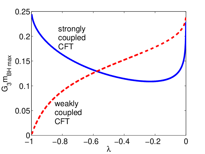
In Figure (5), we plot the strongly and weakly coupled CFT parameters and respectively versus the black hole mass for small and large values of , or equivalently for low and high background temperatures reminding that . In both cases and are increasing functions of . However, for small we find that SCFTBH space closes up (the two zeros and coincides) at a smaller value of compared to that of WCFTBH. This happens when or approaches the critical value . In the same figure, we see that for small values of SCFTBH has larger proper horizon circumference than WCFTBH. This matches exactly what one would find in the case of the D static black hole constructed previously in [17] by cutting a AdS C-bulk having with a critical brane. Once again, as one approaches the critical number , the two zeros and converge to the same value which results in divergent horizon circumference. For , the weakly and strongly coupled solutions exchange their behavior to find that the space of the former closes up and hence its horizon circumference diverges at smaller values of . The transition from small to large regime happens at () as can be seen in figure (6) where we plot the maximum allowed black hole mass, before a naked singularity is formed, versus . The maximum possible mass for WCFTBH or SCFTBH can approach at small values of the background temperature. This result is expected since is the maximum mass a static black hole can have in D. The maximum mass decreases monotonically with the temperature in the case of WCFTBH until a black hole ceases to exist when . In contrast, there is a minimum of at () in the case of SCFTBH. Beyond this temperature, the maximum mass increases until it reaches again at . This is a striking difference between weakly and strongly coupled CFT.

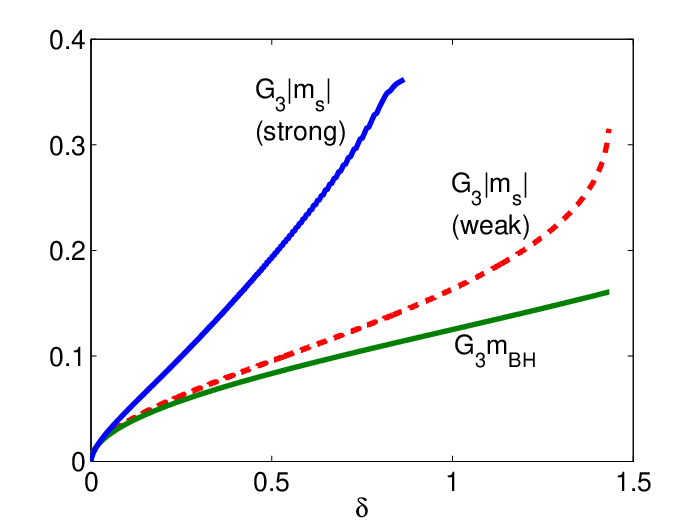


In figure (7), we plot the absolute value of the classical tension , and quantum corrected tension , given in (37), for both strongly and weakly coupled CFT black holes. The behavior of is qualitatively similar to as we find that the absolute value of the former increases with the black hole mass until it reaches a maximum value of . Further increase of results in moving the position of the strut closer to and hence decreasing the value of until the space closes up when . We also see that the absolute value of the quantum corrected tension is larger than the classical one for small values of the black hole mass, which is more evident in the case of strongly coupled CFT. This shows that the CFT is attractive for small values of : although gravity is not dynamical in D, the quantum corrections generate attractive force that tries to decelerate the black hole. Hence, one needs to increase the strut tension to compensate for the attractive force. The picture is reversed for large values of where we find that the CFT, instead, generates repulsive force. This can be understood by computing the mass of the strut as we show below.
The mass of the quantum corrected strut reads , where is the strut proper length
| (50) |
From figure (7) , we see that contrary to the classical case where , the quantum corrections renormalize the strut mass and hence violates this equality. Now, for small values of we have and the CFT keeps its attractive nature. However, as we move to larger values of we find , and bearing in mind the negative sign of , the CFT reverses its nature which explains the repulsive force for large values of .
8 Discussion and conclusion
In this work, we have studied the CFT corrections to two accelerating masses moving with acceleration , by means of a strut connecting them, in a flat background. To achieve this, we first computed the thermal Green’s function for a conformally coupled scalar. This function describes the quantum fluctuations of a quantum field kept in equilibrium with a thermal bath at temperature , which is the Hawking-Unruh temperature associated with the acceleration horizon. In calculating the Green’s function, we used two different boundary conditions, namely, transparent and Dirichlet boundary conditions. We have found that the induced energy-momentum tensor diverges at the location of the strut in the case of Dirichlet boundary conditions, while the same quantity is regular for transparent boundary conditions. Further, we proceeded using the regular form of the energy-momentum tensor to calculate the gravitational backreaction on the spacetime. Interestingly enough, we have shown that the backreaction of the CFT reproduces the same metric found before in [21] which was constructed by cutting the spacetime with angular dependent critical brane. Although the former solution describes accelerated black hole dressed with weakly coupled CFT (WCFTBH), the latter, according to AdS/CFT+gravity, should describe a black hole dressed with strongly coupled CFT (SCFTBH). This is the first use of the duality in a system containing two interacting particles. Moreover, the presence of the CFT at finite temperature gave us an opportunity to study the finite temperature effects in a strongly coupled system.
The existence of the brane implies that high energy states in the dual CFT theory are integrated out, and hence the CFT has a UV cutoff scale , or in terms of the number of CFT degrees of freedom and the D Newton’s constant . The solution given by (40) describes a genuine black hole if the Compton’s wavelength satisfies , where is the black hole horizon, otherwise quantum effects would smear it over a volume larger than the horizon radius. As was shown in [22], this requirement sets a new scale on the brane. In other words, a black hole solution is reliable if its mass ranges in . The maximum black hole mass is equal to the maximum mass one can place in D in the case of a static black hole. However, we found that is temperature dependent, and can be determined when the strongly or weakly coupled CFT parameters, and respectively, reaches the critical value . As was shown in figure (6), this mass starts at at low temperatures for both SCFTBH and WCFTBH, and then decreases monotonically until a black hole ceases to exist as in the case of WCFTBH. In contrast to this behavior, for SCFTBH develops a minimum and then increases until it reaches again at . This is a striking deference between strongly and weakly coupled CFT. Nevertheless, in both cases as the black hole mass reaches the maximum allowed value, the proper horizon circumference grows indefinitely. Beyond, the black hole horizon disappears leaving behind undressed singularity in a clear violation of the quantum cosmic censorship. In fact, it was shown in [21] that the time-dependent solutions obtained there do not respect the quantum censorship, as well. Indeed, these results may indicate that the censorship operates only for a static CFT.
The presence of a naked singularity may signal phase transition on the bulk side. However, at this point, it is safe to say that a complete understanding of the nature of this singularity is still an open question. Further study of SCFTBH may reveal rich phenomena of finite temperature CFT coupled to gravity in D.
Acknowledgement
The author is grateful to Lorenzo Sorbo for invaluable help and patience during this work, and to David Kastor for enlightening discussions. The author would like also to thank Yulia Smirnova for her careful reading of a previous version of the manuscript. This work has been supported by the U.S. National Science Foundation under the grant PHY-0555304.
Appendix A: Mass calculations
In this appendix, we calculate the mass of the particles and strut as measured by a static observer sitting in Minkowskian background. We start from the coordinate transformations given in (2) which bring the metric in (1) to the form . Further, we introduce the deficit parameter and require that , and . These transformations cover only the portion of space . To cover the whole space we take and , and demand that , and , where the parameter is defined as . Now, taking the limit we obtain
| (A1) |
This describes two point particles moving along the hyperbola , as shown in figure (8). In other words it describes two point particles accelerating in the plane , with acceleration , in two opposite directions. In order to complete the picture, we need to understand the role of the deficit parameter in the coordinates. This can be achieved by eliminating and using the set of transformations given in (1) to find
| (A2) |
which describe two circles, in the plane, with origin located at and radius . A sketch of the loci of the circles is provided in figure (8). For small values of , the intersection region is small, and the final space is constructed by removing this region and gluing the two curves and taking . Hence, the strut is interpreted as the curve or equivalently the curve . This strut stretches between the points and where the two circles intersect. These points move along the hyperbola described above and hence we can assign point particles at the location of these points. As we tune to higher values, the size of the intersection region increases until . At this value of , the two circles coincide. For , the blue and the red circles in figure (8) exchange their positions, and the space in this situation is constructed by removing the region , and then gluing the curves and , until the space disappears when . In summary, we have two point particles located at and which are accelerated by means of a strut stretched between them and pushing them away. Since mass in D is interpreted as missing space, this configuration is realized by removing the region for or for shown in figure (8). In the following, we perform the calculations assuming . However, the results are valid even for .


The length of the arc (or equivalently ) at time can be calculated easily from the geometry of figure (8) to find
| (A3) |
Moreover, we have shown in section 2 that the strut tension, which is a Lorentz invariant, is given by . Hence, we find that the strut mass, , reads
| (A4) |
which is exactly what we have found in section 2 working in the coordinates. From the point of view of an observer in the coordinates, the length of the strut and hence its mass will increase with time. However, an observer moving with one of the point particles, at or , will conclude that the mass of the strut is constant according to her sticks and clocks.
On the other hand, the mass of the point particles located at or can be determined, according to our observer, by measuring the circumference of a circle with radius centered at or , and further dividing the result by to get the total angle enclosed . Then, the mass is given by . To this end, consider a circle of radius centered at point at time
| (A5) |
This circle intersects (A2) in where
| (A6) |
and . Using simple geometric calculations we find that the angle between the positive -axis and the location of is given by
| (A7) |
In the limit we obtain
| (A8) |
and hence the total angle enclosed by the circle is , and the particle mass is given by
| (A9) |
Hence, we find as was shown in section 2. This can be justified by enclosing the geometrical construction by very large circle at infinity to find that the total deficit angle is actually zero.
Appendix B: Properties of associated Legendre functions
In this appendix, we summarize the main properties and relations of associated Legendre’s functions used throughout the paper [30, 31, 38]. The associated Legendre equation of degree and order reads
| (B1) |
where we assume . The solutions of this equation are given by and , the associated Legendre’s functions of the first and second kind respectively. For integer values of , we find that the only well-behaved functions at and are and respectively, where . The Wronskian of these functions is given by
| (B2) | |||||
| (B3) |
The associated Legendre’s functions satisfy the addition theorem
| (B4) | |||||
To sum up the series (3) we use the integral representation
| (B5) |
Finally, for one can make use of the identity
| (B6) |
Appendix C: Calculations of the energy-momentum tensor
The energy-momentum tensor is given by the coincidence limit (25). The coincidence limits of the various derivatives in the case of transparent boundary conditions are given by
where
Moreover, using the fact that the two point function satisfies the homogeneous equation outside the singularity we get the consistency condition . Now, substituting the relations () in eq. (25) we obtain the energy-momentum tensor
| (C3) |
One can follow the same procedure above to obtain in the case of Dirichlet boundary conditions
| (C4) |
where
| (C5) | |||||
References
- [1] L. Randall and R. Sundrum, “An alternative to compactification,” Phys. Rev. Lett. 83, 4690 (1999) [arXiv:hep-th/9906064].
- [2] A. Chamblin, S. W. Hawking and H. S. Reall, “Brane-world black holes,” Phys. Rev. D 61, 065007 (2000) [arXiv:hep-th/9909205].
- [3] R. Emparan, “Exact gravitational shockwaves and Planckian scattering on branes,” Phys. Rev. D 64, 024025 (2001) [arXiv:hep-th/0104009].
- [4] N. Kaloper and L. Sorbo, “Locally localized gravity: The inside story,” JHEP 0508, 070 (2005) [arXiv:hep-th/0507191].
- [5] A. Chamblin, H. S. Reall, H. a. Shinkai and T. Shiromizu, “Charged brane-world black holes,” Phys. Rev. D 63, 064015 (2001) [arXiv:hep-th/0008177].
- [6] H. Kudoh, T. Tanaka and T. Nakamura, “Small localized black holes in braneworld: Formulation and numerical method,” Phys. Rev. D 68, 024035 (2003) [arXiv:gr-qc/0301089].
- [7] N. Dadhich, R. Maartens, P. Papadopoulos and V. Rezania, “Black holes on the brane,” Phys. Lett. B 487, 1 (2000) [arXiv:hep-th/0003061].
- [8] C. Galfard, C. Germani and A. Ishibashi, “Asymptotically AdS brane black holes,” Phys. Rev. D 73, 064014 (2006) [arXiv:hep-th/0512001].
- [9] S. Creek, R. Gregory, P. Kanti and B. Mistry, “Braneworld stars and black holes,” Class. Quant. Grav. 23, 6633 (2006) [arXiv:hep-th/0606006].
- [10] M. Anber and L. Sorbo, “Two gravitational shock waves on the brane,” JHEP 0710, 072 (2007) [arXiv:0706.1560 [hep-th]].
- [11] T. Tanaka, “Classical black hole evaporation in Randall-Sundrum infinite braneworld,” Prog. Theor. Phys. Suppl. 148, 307 (2003) [arXiv:gr-qc/0203082].
- [12] A. L. Fitzpatrick, L. Randall and T. Wiseman, “On the existence and dynamics of braneworld black holes,” JHEP 0611, 033 (2006) [arXiv:hep-th/0608208].
- [13] T. Tanaka, “Implication of Classical Black Hole Evaporation Conjecture to Floating Black Holes,” arXiv:0709.3674 [gr-qc].
- [14] N. Tanahashi and T. Tanaka, “Time-symmetric initial data of large brane-localized black hole in RS-II model,” JHEP 0803, 041 (2008) [arXiv:0712.3799 [gr-qc]].
- [15] R. Gregory, S. F. Ross and R. Zegers, “Classical and quantum gravity of brane black holes,” arXiv:0802.2037 [hep-th].
- [16] R. Gregory, “Braneworld black holes,” arXiv:0804.2595 [hep-th].
- [17] R. Emparan, G. T. Horowitz and R. C. Myers, “Exact description of black holes on branes,” JHEP 0001, 007 (2000) [arXiv:hep-th/9911043];
- [18] R. Emparan, G. T. Horowitz and R. C. Myers, “Exact description of black holes on branes. II: Comparison with BTZ black holes and black strings,” JHEP 0001, 021 (2000) [arXiv:hep-th/9912135].
- [19] J. F. Plebanski and M. Demianski, “Rotating, charged, and uniformly accelerating mass in general relativity,” Annals Phys. 98, 98 (1976).
- [20] W. Kinnersley and M. Walker, “Uniformly accelerating charged mass in general relativity,” Phys. Rev. D 2, 1359 (1970).
- [21] M. Anber and L. Sorbo, “New exact solutions on the Randall-Sundrum 2-brane: lumps of dark radiation and accelerated black holes,” arXiv:0803.2242 [hep-th].
- [22] R. Emparan, A. Fabbri and N. Kaloper, “Quantum black holes as holograms in AdS braneworlds,” JHEP 0208, 043 (2002) [arXiv:hep-th/0206155].
- [23] T. Souradeep and V. Sahni, “Quantum effects near a point mass in (2+1)-Dimensional gravity,” Phys. Rev. D 46, 1616 (1992) [arXiv:hep-ph/9208219].
- [24] H. H. Soleng, “Inverse Square Law Of Gravitation In (2+1) Dimensional Space-Time As A Consequence Of Casimir Energy,” Phys. Scripta 48, 649 (1993) [arXiv:gr-qc/9310007].
- [25] P. R. Anderson, R. Balbinot and A. Fabbri, “Cutoff AdS/CFT duality and the quest for braneworld black holes,” Phys. Rev. Lett. 94, 061301 (2005) [arXiv:hep-th/0410034].
- [26] L. Grisa and O. Pujolas, “Dressed Domain Walls and Holography,” JHEP 0806, 059 (2008) [arXiv:0712.2786 [hep-th]].
- [27] O. Pujolas, “Strongly Coupled Radiation from Moving Mirrors and Holography in the Karch-Randall model,” arXiv:0809.0005 [hep-th].
- [28] S. Deser and R. Jackiw, “STRING SOURCES IN (2+1)-DIMENSIONAL GRAVITY,” Annals Phys. 192, 352 (1989).
- [29] G. Grignani and C. k. Lee, “STATIONARY SOLUTIONS IN (2+1)-DIMENSIONAL GRAVITY WITH STRING SOURCES,” Annals Phys. 196, 386 (1989).
- [30] “Bateman Manuscript Project: Higher Transcendental Functions,“ ed. A Erdelyi, McGraw-Hill, New York, 1953
- [31] Philip M. Morse, Herman Feshbach, “Methods of Theoretical Physics,” McGraw-Hill Science/Engineering/Math, June 1, 1953
- [32] Michel Le Bellac, “Thermal Field Theory,” Cambridge University Press, October 2000
- [33] M. Banados, C. Teitelboim and J. Zanelli, “The Black hole in three-dimensional space-time,” Phys. Rev. Lett. 69, 1849 (1992) [arXiv:hep-th/9204099].
- [34] A. R. Steif, “The Quantum stress tensor in the three-dimensional black hole,” Phys. Rev. D 49, 585 (1994) [arXiv:gr-qc/9308032].
- [35] G. Lifschytz and M. Ortiz, “Scalar field quantization on the (2+1)-dimensional black hole background,” Phys. Rev. D 49, 1929 (1994) [arXiv:gr-qc/9310008].
- [36] K. Shiraishi and T. Maki, “Quantum Fluctuation Of Stress Tensor And Black Holes In Three-Dimensions,” Phys. Rev. D 49, 5286 (1994).
- [37] Milton Abramowitz and Irene A. Stegun, “Handbook of Mathematical Functions with Formulas, Graphs, and Mathematical Tables,“ Dover Publications, 1965
- [38] Chester Snow, ”The hypergeometric and Legendre functions with applications to integral equations of potential theory,“ National Bureau of Standards, 1942
- [39] N. D. Birrell and P. C. W. Davies, “Quantum Fields In Curved Space,” Cambridge, Uk: Univ. Pr. ( 1982) 340p
- [40] G. Kennedy, R. Critchley and J. S. Dowker, “Finite Temperature Field Theory With Boundaries: Stress Tensor And Surface Action Renormalization,” Annals Phys. 125, 346 (1980).
- [41] H. Farhoosh and R. L. Zimmerman, “Killing Horizons And Dragging Of The Inertial Frame About A Uniformly Accelerating Particle,” Phys. Rev. D 21, 317 (1980).
- [42] J. L. Petersen, “Introduction to the Maldacena conjecture on AdS/CFT,” Int. J. Mod. Phys. A 14, 3597 (1999) [arXiv:hep-th/9902131].