The Weibull-Geometric Distribution

Several distributions have been proposed in the literature to model lifetime data. Adamidis and Loukas (1998) introduced the two-parameter exponential-geometric (EG) distribution with decreasing failure rate. Kus (2007) introduced the exponential-Poisson distribution (following the same idea of the EG distribution) with decreasing failure rate and discussed various of its properties. Marshall and Olkin (1997) presented a method for adding a parameter to a family of distributions with application to the exponential and Weibull families. Adamidis et al. (2005) proposed the extended exponential-geometric (EEG) distribution which generalizes the EG distribution and discussed various of its statistical properties along with its reliability features. The hazard function of the EEG distribution can be monotone decreasing, increasing or constant.

The Weibull distribution is one of the most commonly used lifetime distribution in modeling lifetime data. In practice, it has been shown to be very flexible in modeling various types of lifetime distributions with monotone failure rates but it is not useful for modeling the bathtub shaped and the unimodal failure rates which are common in reliability and biological studies. In this paper we introduce a Weibull-geometric (WG) distribution which generalizes the EG and Weibull distributions and study some of its properties. The paper is organized as follows. In Section 2, we define the WG distribution and plot its probability density function (pdf). In Section 3, we give some properties of the new distribution. We obtain the cumulative distribution function (cdf), survivor and hazard functions and the pdf of the order statistics. We also give expressions for its moments and for the moments of the order statistics. The estimation by maximum likelihood using the algorithm EM is studied in Section 4 and inference is discussed in Section 5. Illustrative examples based on real data are given in Section 6. Finally, Section 7 concludes the paper.

The EG distribution (Adamidis and Loukas, 1998) can be obtained by compounding an exponential with a geometric distribution. In fact, if $X$ follows an exponential distribution with parameter $\beta Z$, where $Z$ is a geometric variable with parameter $p$, then $X$ has the EG distribution with parameters $(\beta,p)$. Since the Weibull distribution generalizes the exponential distribution, it is natural to extend the EG distribution by replacing in the above compounding mechanism the exponential by the Weibull distribution.

For $\alpha>1$, the WG density is unimodal (see appendix A) and the mode $x_{{}_{0}}=\beta^{-1}u_{{}_{0}}^{1/\alpha}$ is obtained by solving the nonlinear equation

The pdf of the WG distribution can be expressed as an infinite mixture of Weibull distributions with the same shape parameter $\alpha$. If $|z|<1$ and $k>0$, we have the series representation

Expanding $\{1-p\,e^{-(\beta x)^{\alpha}}\}^{-2}$ as in (3), we can write (1) as

From the Weibull pdf given before, we have

Hence, some mathematical properties (cdf, moments, percentiles, moment generating function, factorial moments, etc.) of the WG distribution can be obtained using (4) from the corresponding properties of the Weibull distribution.

Let $x=(x_{1},\ldots,x_{n})$ be a random sample of the WG distribution with unknown parameter vector $\theta=(p,\beta,\alpha)$. The log likelihood $\ell=\ell(\theta;x)$ for $\theta$ is

The score function $U(\theta)=(\partial\ell/\partial p,\partial\ell/\partial\beta,\partial\ell/\partial\alpha)^{T}$ has components

The maximum likelihood estimate (MLE) $\widehat{\theta}$ of $\theta$ is calculated numerically from the nonlinear equations $U(\theta)=0$. We use the EM algorithm (Dempster et al., 1977; McLachlan and Krishnan, 1997) to obtain $\widehat{\theta}$. For doing this, we define an hypothetical complete-data distribution with density function

for $x,\beta,\alpha>0$, $p\in(0,1)$ and $z\in\mathbb{N}$. Under this formulation, the E-step of an EM cycle requires the conditional expectation of $(Z|X;\theta^{(r)})$, where $\theta^{(r)}=(p^{(r)},\beta^{(r)},\alpha^{(r)})$ is the current estimate of $\theta$. Using that $P(z|x;\theta)=zp^{z-1}e^{-(z-1)(\beta x)^{\alpha}}\times$ $\{1-pe^{-(\beta x)^{\alpha}}\}^{2}$ for $z\in N$, it follows $E(Z|X;\theta)=\{1+pe^{-(\beta x)^{\alpha}}\}\{1-pe^{-(\beta x)^{\alpha}}\}^{-1}$. The EM cycle is completed with the M-step by using the maximum likelihood estimation over $\theta$, with the missing $Z$’s replaced by their conditional expectations given above. Hence, an EM iteration reduces to

where $\alpha^{(r+1)}$ is the solution of the nonlinear equation

where

An implementation of this algorithm using the software R is given in Appendix B.

For interval estimation and hypothesis tests on the model parameters, we require the information matrix. The $3\times 3$ observed information matrix $J_{n}=J_{n}(\theta)$ is given by

where

Here,

for $(j,k,l,m)\in\{0,1,2\}$ and $i=1,\ldots,n$. Under conditions that are fulfilled for the parameter $\theta$ in the interior of the parameter space but not on the boundary, the asymptotic distribution of $\sqrt{n}(\widehat{\theta}-\theta)\,\,\,\,\mathrm{is\,multivariate\,normal}\,\,\,\,N_{3}(0,K(\theta)^{-1})$, where $K(\theta)=\lim_{n\rightarrow\infty}n^{-1}J_{n}(\theta)$ is the unit information matrix. This asymptotic behavior remains valid if $K(\theta)$ is replaced by the average sample information matrix evaluated at $\widehat{\theta}$, i.e., $n^{-1}J_{n}(\widehat{\theta})$. We can use the asymptotic multivariate normal $N_{3}(0,J_{n}(\widehat{\theta})^{-1})$ distribution of $\widehat{\theta}$ to construct approximate confidence regions for some parameters and for the hazard and survival functions. In fact, an $100(1-\gamma)\%$ asymptotic confidence interval for each parameter $\theta_{i}$ is given by

where $\widehat{J}^{\theta_{i}\theta_{i}}$ represents the $(i,i)$ diagonal element of $J_{n}(\widehat{\theta})^{-1}$ for $i=1,2,3,4$ and $z_{\gamma/2}$ is the quantile $1-\gamma/2$ of the standard normal distribution.

The asymptotic normality is also useful for testing goodness of fit of the three parameter WG distribution and for comparing this distribution with some of its special sub-models via the likelihood ratio (LR) statistic. We consider the partition $\theta=(\theta_{1}^{T},\theta_{2}^{T})^{T}$, where $\theta_{1}$ is a subset of parameters of interest of the WG distribution and $\theta_{2}$ is a subset of the remaining parameters. The LR statistic for testing the null hypothesis $H_{0}:\theta_{1}=\theta_{1}^{(0)}$ versus the alternative hypothesis $H_{1}:\theta_{1}\neq\theta_{1}^{(0)}$ is given by $w=2\{\ell(\hat{\theta})-\ell(\tilde{\theta})\}$, where $\tilde{\theta}$ and $\widehat{\theta}$ denote the MLEs under the null and alternative hypotheses, respectively. The statistic $w$ is asymptotically (as $n\to\infty$) distributed as $\chi_{k}^{2}$, where $k$ is the dimension of the subset $\theta_{1}$ of interest. For example, we can compare the EG model against the WG model by testing $H_{0}:\alpha=1$ versus $H_{1}:\alpha\neq 1$ and the Weibull model against the WG model by testing $H_{0}:\alpha=1,p=0$ versus $H_{1}:{\rm\,\,H_{0}\,\,is\,\,false}$.

In this section, we fit the WG models to two real data sets. The first data set consist of the number of successive failures for the air conditioning system of each member in a fleet of 13 Boeing 720 jet airplanes. The pooled data with 214 observations were first analyzed by Proschan (1963) and discussed further by Dahiya and Gurland (1972), Gleser (1989), Adamidis and Loukas (1998) and Kus (2007). The second data set is an uncensored data set from Nichols and Padgett (2006) consisting of 100 observations on breaking stress of carbon fibres (in Gba).

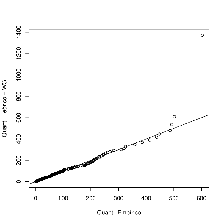
For the first data set, the estimated parameters using an EM algorithm were $\hat{p}=0.7841$, $\hat{\beta}=0.0048$ and $\hat{\alpha}=1.2246$. The fitted pdf and the estimated quantiles versus observed quantiles are given in Figures 4. This figure shows a good fit of the WG model for the first data set.

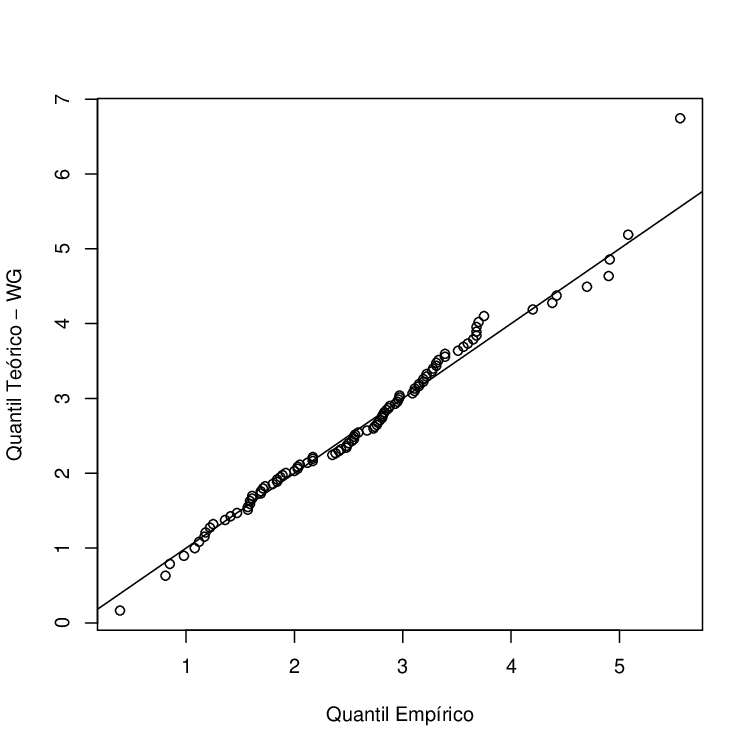
For the second data set, the estimates obtained using an EM algorithm are $\hat{p}=0.3073$, $\hat{\beta}=0.3148$ and $\hat{\alpha}=3.0093$. The plot of the fitted pdf and the estimated quantiles versus observed quantiles in Figure 5 shows a good fit of the WG model.

We define a new model so called the Weibull-geometric (WG) distribution that generalizes the exponential-geometric (EG) distribution introduced by Adamidis and Loukas (1998). Some mathematical properties are derived and plots of the pdf and hazard functions are presented to show the flexibility of the new distribution. We give closed form expressions for the moments of the distribution. We obtain the pdf of the order statistics and provide expansions for the moments of the order statistics. Estimation by maximum likelihood is discussed and an algorithm EM is proposed. We discuss inference, give asymptotic confidence intervals for the model parameters and present the use of the LR statistic to compare the fit of the WG model with special sub-models. Finally, we fitted WG models to two real data sets to show the flexibility and the potentially of the new distribution.

We now show that the WG density is unimodal when $\alpha>1$. Let

When $u\rightarrow 0^{+}$, $h(u)\rightarrow p\frac{\alpha-1}{\alpha}$ and when $u\rightarrow\infty$, $h(u)\rightarrow\infty$. Thus, if $h(u)$ is an increasing function, the solution in (2) is unique and the WG distribution is unimodal. We have $h^{\prime}(u)=1-pe^{-u}\left(u+\frac{\alpha-1}{\alpha}\right)+pe^{-u}$. Using the inequalities $-pe^{-u}\frac{\alpha-1}{\alpha}>-pe^{-u}$ and $-pe^{-u}u>e{-1}$, it follows that $h^{\prime}(u)>1-e^{-1}>0$, $\forall u>0$. Hence, $h(u)$ is an increasing function and the WG distribution is unimodal if $\alpha>1$.

The following R function estimates the model parameters $p$, $\beta$ and $\alpha$ through an EM algorithm.

fit.WG<-function(x,par,tol=1e-4,maxi=100){

# x       Numerical vector of data.

# par Vector of initial values for the parameters p, beta and alpha
# to be optimized over, on this exactly order.

# tol Convergence tolerance.

#maxi Upper end point of the interval to be searched.

p<-par[1]
beta<-par[2]
alpha<-par[3]
n<-length(x)
z.temp<-function(){
(1+p*exp(-(beta*x)^alpha))/(1-p*exp(-(beta*x)^alpha))
}
alpha.sc<-function(alpha){
n/alpha+sum(log(x))-n*sum(z*x^alpha*log(x))/sum(z*x^alpha)
}
test<-1
while(test>tol){
z<-z.temp()
alpha.new<-(alpha.sc,interval=c(0,maxi))$root
beta.new<-(n/sum(x^alpha.new*z))^(1/alpha.new)
p.new<-1-n/sum(z)
test<-max(abs(c(((alpha.new-alpha)),
                ((beta.new-beta)),
                ((p.new-p)))))
alpha<-alpha.new
beta<-beta.new
p<-p.new
}
c(p,beta,alpha)
}

References

• [1] Adamidis K, Dimitrakopoulou, T, Loukas S (2005) On a generalization of the exponential-geometric distribution. Statist. and Probab. Lett., 73:259-269
• [2] Adamidis K, Loukas S (1998) A lifetime distribution with decreasing failure rate. Statist. and Probab. Lett., 39:35-42
• [3] Barakat HM, Abdelkader YH (2004) Computing the moments of order statistics from nonidentical random variables. Statistical Methods and Applications, 13:15-26
• [4] Dahiya RC, Gurland J (1972) Goodness of fit tests for the gamma and exponential distributions. Technometrics, 14:791-801
• [5] Dempster AP, Laird NM, Rubim DB (1977) Maximum likelihood from incomplete data via the EM algorithm (with discussion). J. Roy. Statist. Soc. Ser. B, 39:1-38
• [6] Erdelyi A, Magnus W, Oberhettinger F, Tricomi FG (1953) Higher Transcendental Functions. McGraw-Hill, New York
• [7] Gleser LJ (1989) The gamma distribution as a mixture of exponential distributions. Amer. Statist., 43:115-117
• [8] Kus C (2007) A new lifetime distribution. Computat. Statist. Data Analysis, 51:4497-4509
• [9] Nichols MD, Padgett WJ (2006). A bootstrap control chart for Weibull percentiles. Quality and Reliability Engineering International, 22:141-151
• [10] Marshall AW, Olkin I (1997) A new method for adding a parameter to a family of distributions with application to the exponential and Weibull families. Biometrika, 84:641-652
• [11] McLachlan GJ, Krishnan T (1997) The EM Algorithm and Extension. Wiley, New York
• [12] Proschan (1963) Theoretical explanation of observed decreasing failure rate. Technometrics, 5:375-383