, ,
Largest Empty Circle Centered on a Query Line
Abstract
The Largest Empty Circle problem seeks the largest circle centered within the convex hull of a set of points in and devoid of points from . In this paper, we introduce a query version of this well-studied problem. In our query version, we are required to preprocess so that when given a query line , we can quickly compute the largest empty circle centered at some point on and within the convex hull of .
We present solutions for two special cases and the general case; all our queries run in time. We restrict the query line to be horizontal in the first special case, which we preprocess in time and space, where is the slow growing inverse of the Ackermann’s function. When the query line is restricted to pass through a fixed point, the second special case, our preprocessing takes time and space. We use insights from the two special cases to solve the general version of the problem with preprocessing time and space in and respectively.
1 Introduction
Facilities that pollute their surroundings are necessary evils. Our cities and industrial towns need factories, dump grounds, dams, and nuclear power plants. While we cannot eliminate them completely, we would like to locate them far away from human dwellings. The same problem arises on the flip side when locating, for instance, a school far away from high crime areas and polluting facilities. These scenarios have given rise to a well-studied class of problems known as Obnoxious Facility Location. The most basic problem in this class is the Largest Empty Circle problem, which takes a set of points and asks for the largest circle with its center inside the convex hull of and devoid of points in .
In this paper, we study the placement of an obnoxious facility on a region that can be modeled by a line. Consider the obnoxious facility location that arises in disaster relief, in which planes on a linear flight path must drop personnel in the disaster region. They must, however, be dropped far away from points within the region that pose imminent threat. We address this flavor of problems by formulating a query version in which we are allowed to preprocess the disaster region in a reasonable amount of time, and when queried with a flight path, we can quickly provide the best place for dropping relief personnel.
More formally, we study a query version of the Largest Empty Circle problem in which we are given set of points strictly inside . When given a query line , which we sometime parameterize as , we are to compute the largest empty circle (abbreviated as LEC) with its center on and within the convex hull of . The Largest Empty Circle Problem can have multiple solutions, but conventionally requires us to report only one solution. The query version we study can also lead to multiple solutions, so we keep the convention and limit our requirement to one empty circle with the largest possible radius. For ease of treatment, we simply call this the largest empty circle.
The Largest Empty Circle problem was first studied in the late 70s and early eighties. Toussaint [11] gave an result and showed that it can be extended to the case where the center is constrained to lie within a convex polygon. Bose and Wang [3] have shown that time suffices even when the center is to be constrained within a simple polygon. Chew and Drysdale [5] studied the problem when the Voronoi diagram and convex hull are give as part of the input. They showed that the LEC can be computed in time. The query structure we consider, i.e., requiring the center of the circle to be on a query line, is not new either. For instance, Bose et al. [2] provide the smallest enclosing circle in preprocessing time, space and query time. For more information on obnoxious facility location problems, the reader is referred to the survey by Paola [4].
In this paper, we present solutions for two special cases and the general case. It is well known for the classical Largest Empty Circle problem that the center of the LEC will either lie on a Voronoi edge or the convex hull. In Lemma 2.1, we show that this is true even when given a query line, implying that the center is at an intersection of the query line with either a Voronoi edge or the convex hull. A query line can intersect up to Voronoi edges implying that trivial queries based on this insight alone will not suffice in achieving sub-linear query times. The key insight that is novel to this paper is the construction of a 3D structure consisting of hyperbolic arcs such that when the query line is dropped from , the point at which it lands on the structure defines the center of the LEC. The three cases differ in the way we modify the structure so that we can, in time for all cases, compute the landing point (and hence the center of the LEC). This entails finding the upper envelope of a set of functions for which we appeal to the concept of Davenport-Schinzel sequences [6, 7, 10].
In the first special case, we restrict the query line to be horizontal, i.e., of the form , where is a constant. We preprocess it in time and space, where is the slow growing inverse of the Ackermann’s function. When the query line is restricted to pass through a fixed point, the second special case, our preprocessing takes time and space. In both cases, we project the 3D structure consisting of hyperbolic arcs to a 2D plane so that we can find the landing point.
For the general case, we assume without loss of generality that the query line intersects the -axis. In addition, we assume that for any fixed query line, there are at most 3 LECs and consider more than three occurrences to be degenerate. In Section 5 we describe how this degeneracy can be detected and removed. In Lemma 4.1, we show that the -axis can be divided into intervals such that each is an instance of the “query line through a point” case. This easily leads to an time algorithm, but we use persistent data structures [8] to reduce the preprocessing time to with the data structure taking space.
The paper is organized as follows. In Section 2, we provide some initial insights and a high-level framework for solving all cases. In Section 3, we consider the special case in which the query line is guaranteed to be horizontal. The second special case in which the query line goes through a fixed point is addressed in Section 4. Finally, we provide the solution for the general case, i.e., arbitrary query lines, in Section 5.
2 Characteristics of the Solution
It has been known that the center of the LEC lies either on a Voronoi edge or the convex hull of the points in [11]. This notion holds true in our situation also and is captured by the following lemma. Note that since we require the center of the LEC to lie within the convex hull, we only consider portions of the Voronoi edges within the convex hull.
Lemma 2.1
The center of the LEC centered on the query line will be the intersection point of either with a Voronoi edge or the convex hull.
Proof. Let be the center of an LEC centered on . Let be a point closest to . Consider the Voronoi cell enclosing point . The query line must pass through it (or at least touch it at ) because otherwise, will be in some other Voronoi cell and hence closer to some other point in . Let be the point on closest to . The distance from to will be a convex function with its minimum at and strictly increasing on either direction of . Therefore, the point will be as far away from as it can go within the Voronoi cell of and within the convex hull of . This will have to either be a Voronoi edge or the convex hull of . ∎
Lemma 2.1 leads us to the straightforward algorithm of checking all intersections of with the Voronoi edges and the convex hull edges. The convex hull intersections cannot be ignored because in some cases, such as the instance shown in Figure 1, the query line misses all the Voronoi edges inside the convex hull. Note that the convex hull (and the Voronoi diagram) can be constructed during preprocessing in time.


In the preprocessing step, as a consequence of Lemma 2.1, we consider the Voronoi edges and the convex hull as shown in Figure 2. More precisely, we don’t consider the Voronoi edges in full, but rather only those segments that are encompassed by the convex hull. For the sake of convenience, we use the generic term, Voronoi edges, to refer to these internal segments. Additionally, we break the convex hull into segments delimited by points in that are on the convex hull and the points where the Voronoi edges intersect the convex hull. To illustrate, the convex hull in Figure 2 is broken into 19 segments. Note that the number of such segments will be . For the sake of uniformity, we treat all the convex hull segments and the Voronoi edges as a single set . Let be the cardinality of . We construct a 3D structure , where each is a hyperbolic arc corresponding to an . The hyperbolic arcs are subsequently transformed in a manner that will allow us to query in time. Algorithm 1 gives us a high-level framework for preprocessing . While the creation of (line number 2 of Algorithm 1) is common to all versions of the problem that we study, the manner in which the structure is transformed to a form that can be queried (line number 3 of Algorithm 1) is quite different for each version and is progressively more complicated. We explain the construction of in this section and defer the description of the transformations to later Sections.

For each Voronoi edge , we now describe how and why we construct a corresponding hyperbolic arc directly above it as shown in Figure 3. Let and be the two points that induce . For convenience, we consider to be the parameterized representation of the point on that is units from the intersection of the line segment and the (possibly extended) Voronoi edge . Intuitively, each point of the hyperbolic arc is the elevation of the point in the direction to a height that equals the euclidean 2D distance from to either or . Let be the euclidean distance from (or equivalently ) to . The height of the hyperbolic arc corresponding to the point on is equal to the distance . Therefore,
where is the euclidean distance between and . Hence the arc is hyperbolic.
We note that the above description also holds for the convex hull segments in . Each convex hull segment is closest to at most one point because of the way we have segmented the convex hull. This closest point induces the hyperbolic arc the same way the two points induce the arc for Voronoi edges. Note that this hyperbolic arc will be a straight line for those convex hull segments that are incident on a point in the convex hull of . This is a natural consequence of the way we construct the hyperbolic arcs and does not pose a problem to our algorithms.
While Figure 3 shows the construction of the hyperbolic arc on an infinitely long Voronoi edge, our problem is restricted to finding the LEC with center within the convex hull, we will only consider the (finite) edges in . Such finite edges will only induce hyperbolic arcs rather than the full hyperbolas. Note also that each hyperbolic arc can be constructed in time if the points that induce the edge11 1 Of course, the hyperbolic arcs above the convex hull segment are only induced by one point. and the extents of the edge (i.e., the values between which the hyperbolic arc is defined) are given to us.
One way to interpret this structure in light of Lemma 2.1 is to drop our query line from onto the hyperbolic arc structure and report the center for the LEC corresponding to the point at which it touches some hyperbolic arc and projected straight down onto the plane.
3 Horizontal Query Line
In this section, we assume that the query line will be of the form , where is some constant. recall that the points in lie strictly in . The preprocessing is outlined in Algorithm 2.
In step number 3 of Algorithm 2, each point in a hyperbolic arc will be projected (orthographically) onto the point . The orthographic projection preserves the hyperbolic nature of the arcs. Therefore, each hyperbolic arc becomes a hyperbolic arc on the plane. Let . Recall that we are only concerned with the first point at which the query line, , touches the structure when dropped from onto . It is easy to see that this corresponds to the upper envelope curve in at . Hence, we need the upper envelope of . Any two projected hyperbolas in can intersect at a maximum of two points and are partially defined owing to the fact that all hyperbolic arcs in are constructed above the region. Therefore, we appeal to the definition of Davenport-Schinzel sequences and Theorem 3.3 stated by Sharir and Agarwal [10] and restated here in an abridged manner to capture our requirement. (Please refer to the excellent exposition by Sharir and Agarwal [10] for more information about Davenport-Schinzel sequences and their application in finding lower and upper envelopes.)
Definition 3.1
[10] Let be an alphabet with characters and be an integer constant. A sequence , where each , is an Davenport-Schinzel sequence if it satisfies the following conditions:
- 1.
for each , and
- 2.
there do not exist indices , where , such that
and .
Definition 3.2
[10] , where is an Davenport-Schinzel sequence.
Theorem 3.3
Since our hyperbolas meet at 2 points at most, . Further, the hyperbolas are partially defined. Therefore, from Theorem 3.3 and the upper bounds on functions given in [10], we know that , where is the slow-growing functional inverse of the Ackermann’s function. This directly leads us to the following corollary.
Corollary 3.4
The upper-envelope of the set of partially defined hyperbolas , can be computed in .
Proof. In , all the hyperbolas are oriented upward and hence intersect at most at 2 points. Further, since they are partially defined, the proof follows from Theorem 3.3. ∎
The upper envelope of will be a sequence of maximal intervals of -values such that within each interval we have a single function from that dominates. Hence, when we get a query line of the form , we merely search for the interval that contains . This takes time. Let be the edge that induced the hyperbola corresponding to the resulting interval. The intersection of and is the required center of the LEC.
Theorem 3.5
Given a set with points in , we can preprocess in time and space such that when we are given a query line of the form , where , we can report the LEC centered on in time.
4 Query Line Through a Fixed Point
In this section, we study the special case where the query line passes through a pre-specified point called the pivot. Without loss of generality, we assume that the origin is the pivot. We work out the essential details first assuming that ; this restricts the pivot to the bottom left corner. Subsequently, we will show how this can be generalized to .
In this section, we assume that the set of edges and the corresponding set of hyperbolic arcs are already constructed. We say that a query line lands on at angle if it makes an angle with the -axis and an LEC is centered at the intersection of and . In other words, when is dropped from , the hyperbolic arc corresponding to is the first hyperbolic arc it lands on. Drawing from this imagery of the query line landing on hyperbolic arcs, we use the phrases “landing on the edge ” and “landing on the hyperbolic arc ” interchangeably. In case it lands on more than one hyperbolic arc, we simply consider one of them.
Consider an interval such that for all , lands on a hyperbolic arc (or equivalently on the corresponding Voronoi edge ). Extending our previous definition, we say that lands on (or ) in the angular interval .
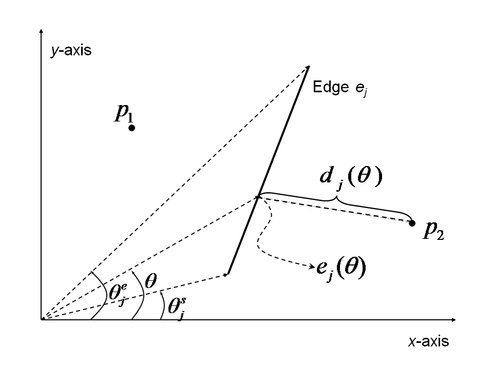
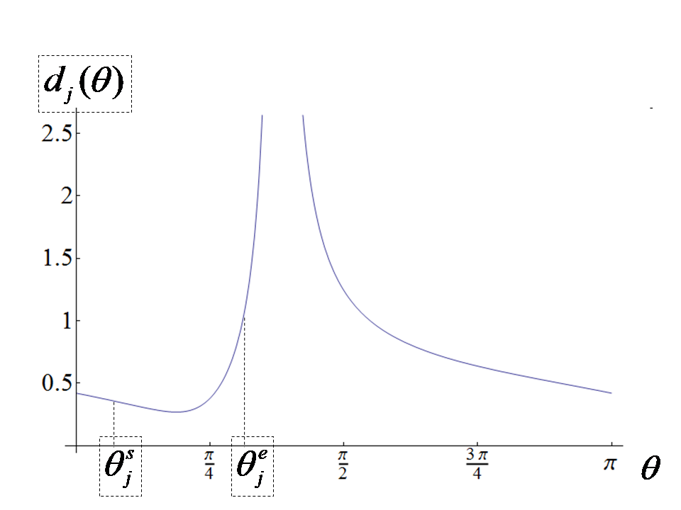
To aid in computing the edge on which a query line lands, we first compute a function for each edge taken individually. We omit the subscript when it is clear from the context. Intuitively, it is the height at which a query line making an angle with the -axis touches the hyperbolic arc constructed over . More precisely, if is the maximal range of angle such that a query line making an angle intersects edge at a point denoted , then
In the above equation, is used to denote the 2D euclidean distance between and .The upper envelope of all these functions, 22 2 We use to denote the supremum over a set of real values, which is defined to be the smallest real value that is greater than or equal to every ., provides us the radius of the LEC given a query line making an angle with the -axis. With some algebraic and geometric manipulations, we get to be of the form
| (4.1) |
where , , , and are constants dependent on the point in that induces the edge .
When given a query line passing through the origin and making an angle , we intuitively “drop” the query line from and consider the first hyperbolic arc it touches. This will be the hyperbolic arc with the largest value. Since the query line can have an arbitrary angle , we compute the upper envelope of the hyperbolic arcs in the preprocessing step. In the query phase, we can search to find the appropriate hyperbolic arc that lands on. Finally, we define the landing sequence of hyperbolic arcs, denoted , to be , to be the sequence of hyperbolic arcs that are encountered as a query line is swept from to .
Lemma 4.1
Given a set of points, each point lying in , and a query line that is restricted to pass through the origin, the landing sequence of is an Davenport-Schinzel sequence consisting of partially defined functions.
Proof. The upper envelope curve that is constructed from the individual curves of the edges in determines the landing sequence. (Note that ). The complexity of in turn depends on the possible number of intersections between any two curves. If we equate the two functions (given in Equation 4.1) and solve the resulting fourth degree equation for , we will get up to 4 roots. Therefore, theoretically we can have at most four angles at which any two functions can intersect. Also, we know that our hyperbolic arcs (and the useful range of the functions) are of limited size. Therefore, the landing sequence will be an Davenport-Schinzel sequence consisting of partially defined functions. ∎
Therefore, from [10], we can construct the upper envelope of the functions for all the hyperbolic arcs (and hence the landing sequence) in time, where is some constant. Since and grows slower than in the asymptotic sense, we can rewrite the running time as and up to an equal amount of space. Although Lemma 4.1 indicates that any two functions intersect at up to 4 points, we have been unable to realize this in an example. We believe that the sequence will in reality be simpler, but we don’t have a proof for it. The preprocessing steps are outlined in Algorithm 3.
Given the upper envelope of the curves and the angles at which the transitions occur in the upper envelope, we can, in time, find the exact hyperbolic arc on which a given query line (passing through the origin and making an angle with the -axis) lands. Substituting the angle in the function for the hyperbolic arc, we can get the radius of the largest enclosing circle. The intersection of the query line with the edge it lands on is the center of the LEC.
4.1 Pivot in Arbitrary Location
So far, we have worked under the assumption that the pivot point, i.e., the point through which the query line must pass, is the origin and the points are in . However, this does not ensure the generality of the solution. In particular, what if the pivot point needs to be inside the convex hull of ? We can address this by placing the points in in . Now, without loss of generality, the pivot can continue to be the origin. We again need to compute the function for each edge in , but this time, we sweep a ray (starting at the origin) about the origin for the entire radians. This will not affect the asymptotic running time adversely because any two functions will again have at most 4 intersections. A consequence of using rays instead of lines for computing the functions is that when the query line makes an angle with the -axis, we have to check the upper envelope at and .
5 Arbitrary Query Line
In this section, we consider the general version of the problem in which the query line can be arbitrary. Recall that we assume that the points are strictly in . Any query line that intersects the convex hull of must also intersect two edges of the square. We assume that our query line intersects the edge on the -axis; we don’t compromise on generality because we can repeat this preprocessing for other edges without any asymptotic increase in time or space.
Our approach for this general version builds on the special case studied in Section 4 where passes through the origin. Like before, we construct a set of hyperbolic arcs in 3D space and seek the point at which lands. We show that the -axis (between ) can be partitioned into maximal segments such that query lines intersecting a given segment induce the same landing sequence. Note that the upper-envelopes will vary depending on the exact point at which intersects the -axis, but we seek maximal segments in which the landing sequence will remain unchanged.
The algorithm described in Section 4 will not suffice because it requires the upper envelope, which lends itself to binary searching. The landing sequence is merely a sequence of hyperbolic arcs. The angular range in which each arc dominates is not included. So it is not possible to determine whether the query line intersects the upper envelope before or after the middle element in any portion of the landing sequence. Therefore we start with a detour to show how the algorithm described in Section 4 can be modified to work with the landing sequence and without the full upper envelope. Subsequently, we show that the landing sequences changes incrementally as the point at which the query line intersects the -axis moves along the -axis. This allows us to store the incrementally changing landing sequences in a persistent data structure, which can be queried in time.
5.1 Querying with the landing sequence
In this section, we show that the algorithm described in Section 4 can be modified to work even when restricted to using the landing sequence alone and not the upper envelope . For binary search to work, we need to ask whether the query line at angle intersects the upper envelope before or after the middle element of the sequence and recurse either left or right according to the response. As mentioned earlier, we cannot answer this question because we don’t know the angle at which the function of each hyperbolic arc in the landing sequence starts to dominate over the previous element in the landing sequence. We overcome this limitation by storing a little more information that neither increases the running time nor the space (in the asymptotic sense).
From the definition, in an Davenport-Schinzel sequence such as the landing sequence, any two elements and can occur in order at most three times. Therefore the consecutive pair can also occur at most 3 times. We call them the meetings of and . Given a pair and and a point on the -axis through which our query line passes, we can find the (at most) three meeting angles at which hands over to in time by simply equating the two functions of and and solving for . Of the four roots and taking the extremities of the partial functions, at most three will correspond to handing over to . Therefore, in the preprocessing phase, we store the meeting number (i.e., either first, second or third) along with each meeting without any increase in the asymptotic running time or space. This allows us to treat the three meetings independently. In Algorithm 3, we add the following line after Line number 4. “Construct the landing sequence from the upper envelope and additionally store the meeting numbers as a separate sequence , where is the meeting number of the pair .”
In the query phase, we perform a binary search on (in conjunction with ) by asking the following question: is the angle that the query line makes with the -axis to the left or right of the th meeting of , where the th meeting of is the central pair in the portion of the landing sequence considered in the current recursion. This can be answered in time, thereby establishing an query time.
5.2 Partitioning the -axis
Let be the landing sequence for query lines passing through . Along the -axis, we encounter several maximal intervals of the form , , during which the landing sequence remains unchanged for all . As we walk along the -axis from to , the landing sequence changes at a finite number of points that we call events. We now ask three questions:
- 1.
what are the possible types of changes that an event can induce in the landing sequence,
- 2.
how many such events exist in , and
- 3.
how do we compute the events?
We address these questions in a series of lemmas. In order to prove these lemmas, we consider the following situation to be degenerate: four or more LECs occur on a single query line. In other words, the degenerate case happens when a ray lands simultaneously on four or more hyperbolic arcs. Subsequently, we will briefly show how to detect and accommodate this degeneracy by slightly perturbing the points in .
We note that similar situations have been studied previously along
with observations that are similar to ours. Bern et al.
[1], for instance, study the changes in the topology
of a 3D scene when viewed along a straight line flight path. Suppose
we walk along the -axis starting from the origin toward in
order to track the changes that we encounter in the landing
sequence. Let be an event point. For some small ,
. Let us first assume that the change is an
insertion of hyperbolic arcs at a single location in the sequence.
We will see that either one or two arcs are inserted. Note that an
insertion when walking in one direction is a deletion when walking
in the opposite direction, hence our assumption does not affect
deletions.
Suppose the sequence of hyperbolic arcs inserted at is .
We can break up and into subparts consisting
of hyperbolic arc sequences (denoted by and ), and
single hyperbolic arcs (denoted by , , and ) in two
possible ways as shown below.
Case A: and , or
Case B: and ,
where “” is the concatenation operator. In other words, is
either inserted in the middle of an existing hyperbolic arc (Case A)
or at the meeting point of two hyperbolic arcs (Case B). Lemma
5.1 provides us the answer to the first
question: what types of changes can we encounter?
Lemma 5.1
If we further divide the cases defined above as shown in the table below, Case A* and Case B* cannot occur for non-degenerate input.
Proof. Cases A1, A2, and B1 are shown schematically in Figures 5, 6, and 7 respectively. Note that each figure highlights a small portion of the the hyperbolic arcs viewed orthographically as explained in Section 4. We prove the impossibility of occurrence of the two cases separately.

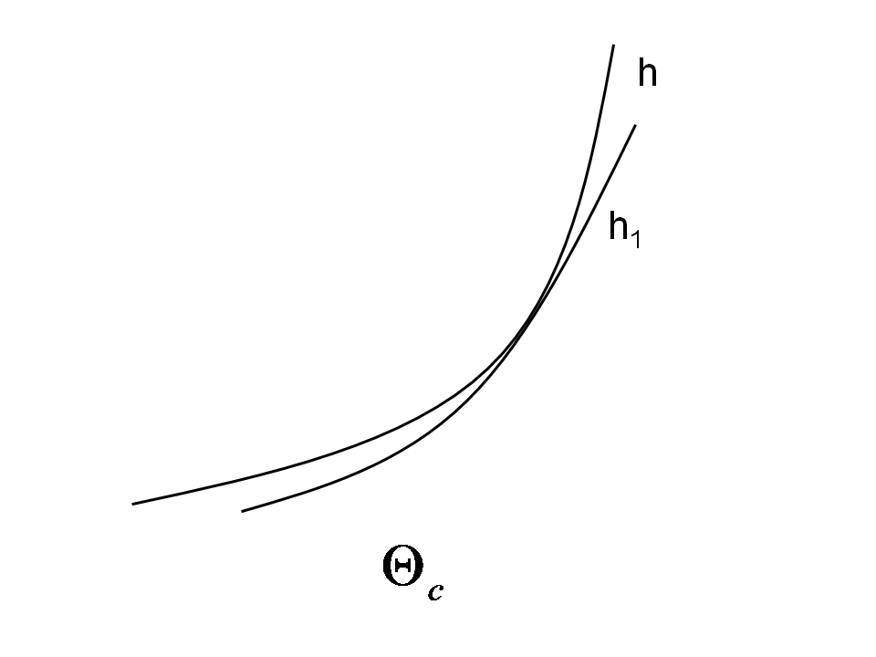
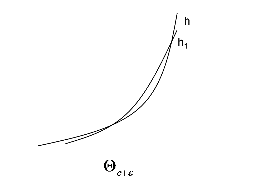


Case A*: In this case, at our event point , three or more hyperbolic arcs that were occluded by the hyperbolic arc (and hence not present in ) appear in . This can happen only if the query line (passing through in 2D) at the appropriate angle, when dropped from , will land on the three (or more) newly appearing hyperbolic arcs and the occluding hyperbolic arc , thereby leading to four or more LECs, the degenerate case.
Case B*: If this case were to occur, two hyperbolic arcs and must be inserted between two other hyperbolic arcs and that were present in . At such an event point , the query line that intersects the -axis at and lands on and will also land on the other two hyperbolic arcs and , thereby leading to four LECs. ∎
We now turn our attention to the second and third questions: how many event points can we encounter on the -axis, and how do we compute them? A natural consequence of Lemma 5.1 is that each event point is defined by either two or three hyperbolic arcs. Lemma 5.2 allows us to compute event points when we consider just two or three edges in a Voronoi diagram. Therefore, in order to construct all the event points, we have to consider all the hyperbolic arc subsets of size two and three.
Lemma 5.2
All event points induced by a subset of hyperbolic arcs containing either two or three arcs can be computed in time.
Proof sketch. For the purpose of this proof sketch, we rely on the orthographic viewing of the hyperbolic arcs. Figure 5 illustrates the interaction of two hyperbolic arcs to induce a change in the landing sequence. With some algebraic and geometric manipulations, we find the point where the hyperbola just appears. In similar fashion, we can find the event point at which the landing sequence changes for cases A2 and B1 also (see Figures 6 and 7). ∎
Lemma 5.3
The number of the events on the -axis from the origin to is and the ordered sequence of events can be computed in time.
Proof. Cases A1, A2, and B1 are all induced by the interaction of either two or three hyperbolic arcs. Therefore, we consider all possible pairs and triples and compute the set of all the events that each pair or triple can induce between . The union of all these sets will give us the set of all events. Since there are triples and fewer pairs and given Lemma 5.2, we can compute the set of all events in time. Therefore, the sorted sequence of events can be computed in time. ∎
In Lemma 5.3, we show that the -axis can be divided into intervals such that each is an instance of the “query line through a point” case. This easily leads to a naive time algorithm in which we store the difference landing sequences, each of length at most . In the query phase, we can find the appropriate landing sequence in time and subsequently search within the landing sequence using the technique described in Section 5.1, again, in time.
We can do better using persistent data structures [8]. We start with a landing sequence at the origin. The sequence takes at most space for the origin. It gets updated at most at each of the event points taken in sorted sequence. When we calculate each event, we also store the update that takes place; each update requires space. In particular, we store the following information:
- 1.
the value at which the event occurs,
- 2.
the sweep angle at which the event occurs,
- 3.
insertion or deletion,
- 4.
the sequence of hyperbolic arcs that are inserted or deleted, and
- 5.
the meeting numbers to ensure that the landing sequences can be searched in time.
For the same reason that the size of the landing sequence is at the origin, the size never gets beyond that at subsequent events. Therefore, with the above information, we can use persistent data structures [8] to store the information in space. For each update, we have to perform an search to find the appropriate location to make the update. There can also be a constant number of updates in the meeting numbers in the sequence. Each could require a binary search, taking time. Therefore, the running time for the preprocessing phase is .
In the query phase, we search for the event point that just preceded the intercept of the query line; this takes time. We lookup the landing sequence induced by the event point, which again takes time. This will also be the landing sequence at the intercept. Armed with the landing sequence, we binary search in time to find the exact hyperbolic arc on which the query line lands. This leads us to our final result:
Theorem 5.4
Given a set of points in , we can preprocess it in time and space such that when presented with an arbitrary query line , we can report the LEC centered on and within the convex hull of in time .
We stated earlier that we consider the case where more than three LECs occur on a query line to be degenerate. This is an essential requirement for Lemma 5.1. It can be detected when we consider pairs and triples of hyperbolic arcs to compute the event points. If more than one event occurs at the same point, say on the -axis, and at the same angle, we can conclude that this degeneracy has occurred. We can avoid this degeneracy by slightly perturbing the points in that induce the four or more LECs that cause the degeneracy.
Acknowledgements: We are indebted to M. V. Panduranga Rao and Leo Livshits for discussing useful ideas. We are also grateful to the anonymous reviewers of an earlier manuscript that helped make the current version more readable.
References
- (1) M. W. Bern, D. P. Dobkin, D. Eppstein, and R. L. Grossman. Visibility with a moving point of view. Algorithmica, 11:360–378, 1994.
- (2) P. Bose, S. Langerman, and S. Roy. Smallest enclosing circle centered on a query line segment. Proc. of the Canadian conference on Computational Geometry, pages 167–170, 2008.
- (3) P. Bose and Q. Wang. Facility location constrained to a polygonal domain. Proc. of the Latin American Theoretical Informatics Symposium, pages 153–164, 2002.
- (4) P. Cappanera. A survey on obnoxious facility location problems. Technical Report TR-99-11, Universita Di Pisa, 1999.
- (5) L. P. Chew and R. L. S. Drysdale. Finding largest empty circles with location constraints. Technical Report PCS-TR86-130, Dartmouth College, 1986.
- (6) H. Davenport and A. Schinzel. A combinatorial problem connected with differential equations. American Journal of Mathematics, 87:684–694, 1965.
- (7) J. Hershberger. Finding the upper envelope of n line segments in o(n log n) time. Information Processing Letters, 33:169–174, 1989.
- (8) D. D. S. J. R. Driscoll, N. Sarnak and R. E. Tarjan. Making data structures persistent. Journal of Computer and System Sciences, 38:684–694, 1989.
- (9) D. Knuth. The Art of Computer Programming, Vol. 3: Sorting and Searching. Addison-Wesley, New York, NY, USA, 1973.
- (10) M. Sharir and P. K. Agarwal. Davenport-Schinzel sequences and their geometric applications. Cambridge University Press, New York, NY, USA, 1996.
- (11) G. Toussaint. Computing largest empty circles with location constraints. International Journal of Parallel Programming, 12:347–358, 1983.