The Pólya-Tchebotaröv problemThanks: Supported by DGICYT grant MTM2008-05561-C02-01 and the CIRIT grant 2005SGR00611
Abstract.
We describe the solutions to the problem of identifying the continuum in the complex plane that minimizes the logarithmic capacity among all the continuum that contain a prefixed finite set of points. This description can be implemented numerically and this can be used to improve the estimates on the Bloch-Landau constant and other related problems as the maximal expected lifetime of the Brownian motion on domains of inner radius one or the principal eigenvalue for the Laplace operator on such domains.
2000 Mathematics Subject Classification
Primary1. Introduction and history of the problem
Pólya in [Pól29] discussed the following problem which was suggested to him by Tchebotaröv:
Problem 1.
Given a finite number of points , find the continuum with minimal logarithmic capacity such that .
For any continuum , its complement in the Riemann Sphere, is simply connected, therefore there exists a unique conformal map such that around . Here is called the conformal radius of with respect to . In fact, . This provides an equivalent formulation of Problem 1, which is usually called the outer reformulation of the Pólya-Tchebotaröv problem:
Problem 2.
Given a finite number of points find a conformal map such that and is maximal.
So we are looking for a simply connected domain that contains the origin, it is contained in and such that the density of the hyperbolic metric at the origin is minimal. Such domain will be called an extremal domain and the corresponding conformal map, an extremal map.
The existence of the solution is obvious by a normal family argument. This problem was studied in detail by Laurentiev in [Lau30]. He proved the uniqueness and the basic structure of the solution by the method of variations of the boundary. The structure of the extremal domain is characterized by the following theorem, see [Lau34].
Theorem 1 (Laurentiev).
Given a finite number of points , there exists a unique extremal domain for the problem 2 and it is characterized by the following properties:
- (1)
Each point of the plane belongs to either or .
- (2)
The boundary consists of finitely many simple arcs of analytic curves. The points and are endpoints of distinct arcs. Every point of different from the or either belongs to a unique arc and it is a regular point of , or it is the common end of at least three arcs.
- (3)
To any arc consisting of regular points of there correspond under the conformal mapping two arcs of the same length on the unit circle.
When the last property 3 holds we say that the arcs are harmonically symmetric with respect to the origin and it will be the key property to find a numerical algorithm to determine the solution to the problem mentioned above.
In the proof of this last theorem, Laurentiev assumed that the desired domain is bounded by finitely many simple Jordan arcs. This assumption was removed by Goluzin who used the method of inner variations to prove the following:
Theorem 2 (Goluzin, [Gol46]).
Let be arbitrary given points in . Let be the extremal continuum for Problem 1. Then is the union of the closures of all critical trajectories of the quadratic differential
where are some unknown parameters. The extremal univalent function , with that maximizes must satisfy the following differential equation
Remark 1.
The points correspond to common end points of several arcs. If some point is a common end of arcs, then the term will appear exactly times in the differential equation.
Later we will explain how to use this differential equation to obtain a numerical solution to Problem 2.
Goluzin gave a more general result where the problem is to maximize for any . An account of his work is in [Gol69, Chap. 4]. By using this description and after considerable work, Kuzmina in [Kuz82] computes the extremal domain in the case of three points and in [Fed84] this is extended to four points with a certain symmetry (two of the points must be symmetric with respect to a line that passes by the other two).
Later on, Tamrazov found an explicit solution for the problem of points. The general solution to Problem 2 is, according to [Tam05], of the form
where and are a finite number of points in and is a positive integer. This result does not seem to be completely clear, because the function corresponds to a Schwartz-Christoffel formula, thus is going to be a collection of straight segments (one of them going to ) but, even when we have only three points, in most cases (except of very symmetric ones) the solution to the Pólya-Tchebotaröv problem are not straight lines.
Nevertheless the main idea of Tamrazov paper, that all solutions can be exactly parametrized by a finite planar graph is indeed correct. We will give a different proof of this fact. Our approach although it will not yield an “explicit” formula it will be constructive and it is possible to implement a numerical algorithm that produces an approximation to the solution of the Pólya-Tchebotaröv problem.
On Sections 2 and 3 we prove that all solutions are codified by a “nested partition” which are defined there. This is more convenient for us, although it is completely equivalent to a parametrization by graphs. To each set of points the extremal continuum is in correspondence with a unique “nested partition” of and conversely, each “nested partition” provides a solution. Thus all the combinatorial data of the solution is codified in these partitions.
Once we have a parametrization of all possible solutions we introduce in 4 a numerical algorithm to compute numerically the solutions (i.e. to determine the parameters) to the Pólya-Tchebotaröv problem. We illustrate the method making it explicit in the case of points and points (with a certain symmetry). This last case is particularly interesting because it will be of use for the applications that we had in mind which are developed in Section 5.
The Pólya-Tchebotaröv problem is rather basic, thus it is not surprising that it arises in connection with many other problems. The most evident case is in the estimates of the univalent Bloch-Landau constant, the precise formulation of the problem is in Section 5. This has been exploited in [COC08] where this constant was improved. This work is its natural continuation. Here we will provide more sophisticated examples and we will use the same type of domains to improve the estimates of two other extremal problems that were introduced in [BC94]: the expected lifetime of the Brownian motion in a domain with inner radius one and the estimation of the principal frequency of such domains. For the precise definitions and results, see again Section 5.
There are other potential applications of the Pólya-Tchebotaröv problem which could benefit from our (numerical) solution. For instance the best estimates in the Smale mean value conjecture obtained in [Cra07] rely on the computation of the solution of the problem with three points. We have not pursued improvements on this problem.
Acknowledgment: We are indebted to Àlex Haro for illuminating conversations about the numerical implementation of the algorithm.
2. The parametrization of all solutions
In view of Laurentiev and Goluzin results ,the continuum that is a solution of Problem 1 form a finite planar tree with endpoints in the points . The remaining nodes are of order at least three. This motivates the following definition introduced in [Tam05]:
Definition 1.
A graph is a Pólya-Tchebotaröv graph (PT-graph for short) if it is a finite planar tree with the properties:
- (1)
All sides of the graph are linear segments.
- (2)
There are no nodes of order 2.
- (3)
The sum of the length of all sides is exactly 1/2.
We say that is normalized if we mark one of the vertex of the tree (a node of order one). Two PT-graphs are equivalent if there is an isometry from one to the other that extends to an orientable homeomorphism of the plane. If they are normalized we also require that the isometry sends the marked vertex from the first graph to the marked vertex of the second graph. We will talk of a PT-graph to denote the whole equivalence class.
Since Problem 1 is invariant by translation we can be normalize the data to assume that .
The main result is that there is a natural way of parametrizing the solutions to the Pólya-Tchebotaröv problem by normalized PT-graphs. That is for any graph there is associated a unique continuum that solves a Pólya-Tchebotaröv problem and conversely all solutions arise in this way.
Let us describe how to associate a solution to each graph. First we need one further definition.
Definition 2.
A partition of the unit circle in a finite number of intervals is called a properly nested partition if the following properties hold:
- (1)
The intervals come in pairs of equal length, i.e.
and for all .
- (2)
There are no nested pairs of intervals, i.e. a couple never separates another couple . See Figure 1
Since all pairs are not nested we can be sure that there exist at least one pair of adjacent intervals. Two partitions are equivalent if one rotation sends one to the other. They are normalized if we mark one of the adjacent pairs of intervals.
It is easy to see that any PT-graph provides a nested partition and conversely. We start from a vertex of the graph and travel through its edges directwise. To each edge of the tree we associate an interval in the circle of the same length (on the unit circle we consider the normalized length). Each edge of the tree is visited twice, once for every side. We consider the pairs of intervals to intervals that correspond to different sides of the same edge of the tree.
Finally for any given properly nested partition there is associated an involution defined on the circle (except in a finite number of points corresponding to the end points of the intervals). Two points are related by the involution if belongs to the interval and belongs to its pair . The definition of in each of the intervals is the reflection along the diameter of the disk that passes halfway in between the pair of intervals as in Figure 2
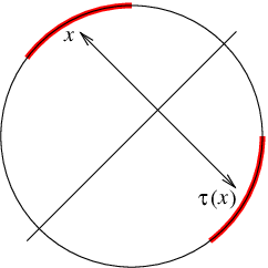
We are going to prove a “welding” type theorem:
Theorem 3.
For any given properly nested partition of and its associated involution there is a conformal map where is a finite union of analytic arcs such that the image of any pair is one arc and for all in the intervals. Moreover is unique up to postcomposition with automorphisms of .
Remark 2.
If we compose with a translation we obtain a function that satisfies the Laurentiev conditions of Theorem 1. Thus for any we get a solution to Problem 2. The converse is even more clear. Laurentiev theorem shows that the boundary of the extremal domain is a tree, that is homeomorphic to a rectilinear PT-graph . The length of each edge of is one half of the harmonic measure of the corresponding edge of . The conformal map with gives a partition of the unit circle. By property (3) of Laurentiev theorem, we get .
3. Proof of the welding Theorem
Given the partition we will proceed to construct the mapping in a finite number of steps. In each step the following lemma is the key
Lemma 1.
Given two adjacent intervals in the circle, such that and a quasisymmetric homeomorphism that fixes the common point , there is a simple Jordan arc with one endpoint at and a conformal mapping such that and for all . The mapping and the curve are unique, they depend on and .
Proof.
Let and , and let be defined as . If these were the data of the problem, it will be readily solved by the mapping that maps to . In the general situation, there exists an homeomorphism of the circle such that , and for all . In , the map is defined linearly. On we use as definition and outside and we define it linearly. Since is asymmetric then is quasisymmetric. In general has the same regularity as . By the Beurling-Ahlfors extension theorem [BA56] there is a quasiconformal homeomorphism of the disk that extends . We will still denote it by .
Let . The map is mapping and to the arc in such a way that for all . It is not a conformal, but it is a quasiconformal map because is quasiconformal and is conformal. This can be corrected by solving a Laplace-Beltrami equation. We want an homeomorphism such that is conformal. Thus . There is always a solution to this Laplace-Beltrami equation that is an homeomorphism from to since almost everywhere by the measurable Riemann mapping theorem. Finally we compose with an automorphism of the disk and the desired function is . The automorphism is chosen to make sure that and the endpoint of is at . The regularity of at the boundary is as good as that of and that itself is determined by the regularity of .
If there were two curves and and two maps and with the same property then is a conformal mapping from to such that . Moreover extends continuously to because for any point in the preimage by are two points in that are related by , thus , therefore extends continuously to and therefore it extends analytically, thus . Since both and start have an endpoint in , then and . ∎
With the same proof, mutatis mutandi, we deal with the case and we obtain
Lemma 2.
Given two adjacent intervals in the circle, such that and a quasisymmetric homeomorphism that fixes the common points, there is a simple Jordan arc with one endpoint at and the other at and a conformal mapping such that , and for all . The mapping and the curve are unique, they depend on and .
Proof of the theorem.
We take any pair of adjacent intervals in the partition corresponding by the involution . There are always adjacent pairs because the partition is properly nested (they correspond to edges with and endpoint in a vertex of the graph). Applying the Lemma we find a conformal mapping that welds together the pair of intervals in a curve . The mapping induces a new partion of , and for all except for the pair that was welded together. This new partition is again correctly nested because the order is preserved except for a pair of adjacent intervals that “collapses”. The number of pairs of intervals is one less than in . The intervals in each pair are no longer of the same size but nevertheless the map induces a new involution on them, .
Now we repeat the procedure. We take any other new pair of adjacent of intervals of the new partition corresponding by and we glue them together. This can be done by a mapping applying the Lemma because is quasisymmetric (it is in fact piecewise real analytic). In this way we get again a new involution and a new nested partition .
In this way we keep gluing pairs of intervals until we are left only with two intervals and an involution that relates them. In this last step we use Lemma 2 to get . The final conformal mapping is .
There is basically only one such map (except for composition with maps of the form ). The proof is as in Lemma 1, suppose there is another such map . Let , then is a one to one analytic mapping . Moreover since the preimage of any regular point in are two points in the circle that are related by the involution, and maps both points to the same point, then can be extended continuously to a conformal map from to , thus . ∎
4. Numerical Algorithm to find solutions
As we mentioned above, in order to implement numerically an algorithm to find the solution to Problem 2, we used an important property of the extremal domain and the differential equation obtained by Laurentiev. Denote by the desired extremal domain for the Problem 2 in case of points . Let be the conformal map such that . We know that satisfies the following differential equation
| (1) |
where the parameters are unknown and . Using the solutions of this differential equation and the last property of Theorem 1 we have implemented the resolution of Problem 2 for some cases of . The system becomes more delicate as increases, the combinatorics and the dimensions of the systems to solve become bigger. We will show in detail the solution in the case to illustrate the method and with some extra symmetry, because this will be enough for the applications that we have in mind. The code where this algorithm is implemented (for four points and 6 points with symmetry) can be downloaded from http://www.maia.ub.es/cag/code/tchebotarev/.
4.1. Case of 3 points
Let’s start with 3 points. Assume that we have three points such that and . Without loss of generality we will always assume that . In the case of three points the extremal domain is very clear (see Figure 3). We only have one unknown parameter denote it by in the differential equation (1) that reduces to:
| (2) |
Recall that to any regular arc of there corresponds two arcs with equal lengths on the unit circle. So this means that we have the configuration on the unit circle shown in Figure 4,
where , the arcs are mapped to the arc , and are mapped to the arc and the arcs into . Note that for and for .
The solution of the problem can be viewed as the solution of a system of non-linear equations. If we know the value of and we can compute the coefficients of the mapping using the differential equation (2). We computed also the values of . Note that as the arcs , must have same length, we get (we will always take the angles in the range ). So, we have 6 real unknown parameters in our problem: and using the last property of Theorem 1 we can impose the following three complex equations
We used a the hybrid method to find an approximation of the roots of the system (see [Pow70] for more details of the method).
To apply the root-finding method we need to evaluate for any . For that, denote . We know that and . Note that . We can get the differential equation satisfied by and solve it to obtain the value in time . We get
| (3) |
Note that this equation only defines up to a sign, we will deal with this problem by analytic continuation. Once we fix the derivative at the origin there is a single analytic branch that solves the equation. To solve it we used the Taylor integration method which allows us to integrate the singularity in . As is conformal, we know that , where . Now if we do the calculations in the equation (3) we get a recurrence for the coefficients till the order we want. Now we can estimate the radius of convergence of the obtained series. And therefore proceed using Taylor method to integrate the differential equation until . Hence we will be able to impose the equations to solve our problem.
4.2. Case of 6 points with symmetry
Now consider the case of points such that , and . The extremal compact in this case may be of two types (see Figures 5, 6 and 7).

So, we have two type of configurations in this special case
- (1)
- (2)
,
where for and , for and . Using the symmetry we can do some reductions to get a system of equation with less dimension. For example, we can always assume that the point , so that for the first configuration and for the second one. Note that in this last configuration, by the symmetry of the problem, . Moreover as this is a symmetric case, must be real and .
First configuration
In this case we have real unknown parameters: , , , , , , and we can impose the following equations
Second configuration
We have real unknown parameters: , , , , , , , and we can impose the following equations
In Figures 6 and 7 we show an extremal domain for some 6 points for each configuration. As in the last case, these figures represent a conformal map from the complement of onto such that .


Remark 3.
Note that the solution of the problem depend continuously on the parameters , so if we have one solution for some given set points we can do continuation to reach to any other set of points (with the same topological configuration). This has been used and we did the classic continuation (i.e. for the new set of points we take as a initial condition the solution of the last set of points).
Remark 4.
In the implementation of the method, we found a problem when the distance between the arcs on the unit circle is very small, we can’t integrate properly the differential equation because we are near the poles . However this can be overcome by a change of variables. This has been implemented for the special case of the first configuration mentioned in the case of 6 points. In fact, for the application of the Pólya-Chebotarev we only needed the values of . This data is enough to obtain the expansion in series of the mapping . This can be done in the following way: given the points , we have an initial guess for the unknown values. So, we compute the critical orbit starting at point till the point with imaginary part equal to and same for the critical orbit starting at . The real part of the two points obtained should match if , are the desired solution. So this is one real equation. Same can be done for the couple of points and . So we have two real equations. The last equation can be (this is valid if the points are a bit far from the point ).
5. Applications of the Pólya-Tchebotaröv problem
The fundamental frequency of a domain
In 1965, Endre Makai (see [Mak65]) proved the following theorem solving a problem in the study of vibrating membranes raised by Pólya and Szegö in their book [PS51]. In 1978, Hayman ([Hay78]) unaware of it, reproved the same result.
Theorem 4.
Let be a simply connected domain in the complex plane. Let be the inradius of , that is, the radius of the largest disc contained in and let be the first Dirichlet eigenvalue for the Laplacian in . There is a universal constant such that
| (4) |
There have been many efforts to find the best constant and to identify the extremal domain for . Makai’s proof also shows that the best satisfies .
The following lemma is useful for giving upper bounds for this constant (see [BC94, Lemma 1.2] for a proof):
Lemma 3.
Let be the first Bessel function and the smallest positive zero of . Assume that is a simply connected domain. Then
where
and the infimum is taken over all conformal mappings from the unit disc onto .
In [BC94] Bañuelos and Carroll proved that and provided examples of domains which are close to the extremal domain. They did this relating this problem to two other extremal problems:
The expected lifetime of a Brownian motion
Let be the Brownian motion in . Let be the first exit time of from . Let us denote by the expectation of under the measure of the Brownian starting at the point in . It is known that there is a universal constant such that, whenever is a planar simply connected domain,
| (5) |
As before, we want to know the best value of and the extremal domain for this last inequality. It is a fact that if denotes the unit disc of radius then . It is known that (see [BC94]). In order to give an improved lower bound for it is useful to know the following result (see [BC94, Lemma 1.1.] for further details):
Lemma 4.
Suppose that is a conformal mapping from the unit disc onto a simply connected domain with . Then
The univalent Bloch-Landau constant
If is an analytic and one to one mapping from the unit disc, then there exists a universal constant such that
| (6) |
This means that the image of the unit disc under any conformal map contains discs of radius less that . Note that from Koebe’s 1/4-theorem, we know that . The best value of is known as the univalent or schlicht Bloch-Landau constant. We can reformulate this problem in terms of the density of the hyperbolic metric. If is a conformal mapping from the unit disc such that then the density of the hyperbolic metric is . So we have the following inequality
| (7) |
where . From many years there have been efforts to find bounds for . This constant was introduced in 1929 by Landau [Lan29], who proved that . Reich improved this bound in [Rei56] () and Jenkins in [Jen61] gave . Many other gave some improved bounds. There are many domains proposed as the candidate for the extremal domain in order to obtain upper bounds for the Bloch-Landau constant. For example, Robinson in [Rob35] proved that , Goodman in [Goo45] that and in [BH85] Beller and Hummel proved that . Finally in [COC08] this bound has been improved to . In this last result the resulting domain had all the inner boundary harmonic symmetric with respect to the origin, see Figure 8.

We will use a slight modification of this last domain, which is still harmonic symmetric, to give an improved bound of the Bloch-Landau constant.
As a normalization, we will take domains with inradius 1. We will give improved bounds for the constants appearing in the three problems explained above.
Bañuelos and Carroll in [BC94] conjectured that the extremal domain is the same for all the three problems. When we restrict these problems to the class of convex domains this is true. In our work, we will see that a similar domain improves the bounds for all the three problems.
5.1. Bloch-Landau constant
If is a mapping of the complement of a compact set onto the complement of the closed unit disc, it can be expanded (up to a rotation) as
So we can relate the problem of the extremal domain for the Bloch-Landau constant with Problem 2 in the case of 6 points because minimizing the capacity is equivalent to increasing the derivative at the origin. It is known (see [Car08]) that the arcs making up the extremal configuration must be harmonically symmetric at infinity. We will work with domains as in Figure 9 where is bigger than 4 and we chose the arcs so that this domain is harmonically symmetric with respect to 0.

If is a conformal map of onto with then is a conformal map of onto the domain shown in Figure 10. The arcs in this last domain are harmonically symmetric. We can compute the derivative of at 0: . We need this domain to have inradius 1. Later on we will explain the construction of the domain and the way to get inradius 1.

Let be the Koebe mapping from the unit disc onto the complex plane slit along the negative real axis from minus infinity to -1/4.
Proposition 1.
Let be the conformal map of onto such that . Then taking and ,
where and is the continuum with minimal capacity containing 6 given points with symmetry (see Figure 11).

Proof.
Using the above notations, consider the map
which maps onto the complement of the continuum with and (). Note that the harmonic symmetry of the arcs are preserved since each mapping can be extended continuously to all internal boundary arcs and the domains involved are symmetric with respect to the real axis. Let be the mapping of the complement of onto the complement of the unit disc. Then we can define the map of onto as
We can calculate the derivative by computing the power series of :
The capacity of can be computed numerically as we explained in 4.2. Now and the proposition is proved. ∎
5.2. Construction of the domain
Now we will explain how to obtain the desired domain in order to have inradius 1 and the derivative as big as possible. In what follows, denotes a disc of radius 1 centered at and .
The domain is constructed in stages. Let be a disc centered at the origin with radius . First we remove from this disc three radial slits that start from the cube roots of the unity. Then, we remove three further slits starting at two times the cube roots of -1 (these are the first two stages of Goodman’s domain). Now, as we need inradius 1 we need to put some point in order to not to have discs of radius bigger than 1. Let and denote by the circle centered at with radius 1. We have to put some point in so that this circle can’t increase. Let be a point in this circle. Denote by the circle of radius 1 tangent to the halfline of argument containing the point . Let be the circle of radius 1, tangent to and to the halfline of argument and denote by the intersection point of and , and the centers of , respectively (see Figure 12).

Now let and be the curves at distance one of and (i.e. given a point , let be the normalized orthogonal vector to , then the corresponding point in the curve is . Let denote the intersection of and . One sufficient condition to have inradius one is . The idea to prove this is to cover all the points so that they can’t be centers of circles (contained in ) with radius bigger than one. Let’s show it when our points are located in the sector between the segment and the halfline of argument . If is a point such that , or (where is the halfline of argument ) then obviously we cant have a circle centered at such point with radius bigger than one. Let and be the discs of radius one centered at the points and , respectively. If then contains one of the points or . Therefore, the region is covered. The only risky region is the one between , , and . But this space is covered by the region delimited by the curves due to the hypothesis (see Figure 13).

5.3. Results
We have computed the bounds for all three problems explained before. To construct the point we move on the real axis and define the point and then . After this all gets determined. So given , first we find the biggest such that , (because the derivative at the origin will increase with the radius ) and after that we compute the bounds of the constants explained in the three problems. The results obtained are:
- (1)
For the Bloch-Landau constant, the best upper bound has been found for and and the improved bound is
The domain obtained is shown in Figure 14.

Figure 14. Domain for the improved upper bound of - (2)
Computing the coefficients of the conformal mapping obtained for the domains , the improved upper bound for the fundamental frequency has been found for and and it is
- (3)
The improved lower bound for the expected life time of a Brownian motion has been found for and and it is
In all the computations the error estimates that we required are of the order of , and we are pretty confident on the correctness of the 10 first digits on the bound, but we have not done a rigorous error analysis.
References
- [BA56] A. Beurling and L. Ahlfors, The boundary correspondence under quasiconformal mappings, Acta Math. 96 (1956), 125–142.
- [BC94] R. Bañuelos and T. Carroll, Brownian motion and the fundamental frequency of a drum, Duke Math. J. 75 (1994), no. 3, 575–602.
- [BH85] E. Beller and J. A. Hummel, On the univalent Bloch constant, Complex Variables Theory Appl. 4 (1985), no. 3, 243–252.
- [Car08] T. Carroll, An extension of Jenkin’s condition for extremal domains associated with the univalent Bloch-Landau constant, Comp. Methods and Function Theory 8 (2008), 159–165.
- [COC08] T. Carroll and J. Ortega-Cerdà, The univalent Bloch-Landau constant, harmonic symmetry and conformal glueing, arXiv:0806.2282v1 [math.CV], 2008.
- [Cra07] E. Crane, A bound for Smale’s mean value conjecture for complex polynomials, Bull. Lond. Math. Soc. 39 (2007), no. 5, 781–791.
- [Fed84] S. I. Fedorov, Chebotarev’s variational problem in the theory of the capacity of plane sets, and covering theorems for univalent conformal mappings, Mat. Sb. (N.S.) 124(166) (1984), no. 1, 121–139.
- [Gol46] G. M. Goluzin, Method of variations in the theory of conform representation, Rec. Math. [Mat. Sbornik] N.S. 19(61) (1946), 203–236.
- [Gol69] G. M. Goluzin, Geometric theory of functions of a complex variable, Translations of Mathematical Monographs, Vol. 26, American Mathematical Society, Providence, R.I., 1969.
- [Goo45] R. E. Goodman, On the Bloch-Landau constant for schlicht functions, Bull. Amer. Math. Soc. 51 (1945), 234–239.
- [Hay78] W. K. Hayman, Some bounds for principal frequency, Applicable Anal. 7 (1977/78), no. 3, 247–254.
- [Jen61] J. A. Jenkins, On the schlicht Bloch constant, J. Math. Mech. 10 (1961), 729–734.
- [Kuz82] G. V. Kuz′mina, Moduli of families of curves and quadratic differentials, Proc. Steklov Inst. Math. (1982), no. 1, vii+231, A translation of Trudy Mat. Inst. Steklov. 139 (1980).
- [Lan29] E. Landau, Über die Blochsche Konstante und zwei verwandte Weltkonstanten, Math. Z. 30 (1929), no. 1, 608–634.
- [Lau30] M. Laurentiev, Sur un problème de maximum dans la représentation conforme., C. R. 191 (1930), 827–829 (French).
- [Lau34] by same author, On the theory of conformal mappings, Trudy Fiz.-Mat. Inst. Steklov. Otdel. Mat. 5 (1934), 159–245 (Russian).
- [Mak65] E. Makai, A lower estimation of the principal frequencies of simply connected membranes, Acta Math. Acad. Sci. Hungar. 16 (1965), 319–323.
- [Pól29] G. Pólya, Beitrag zur Verallgemeinerung des Verzerrungssatzes auf mehrfach zusammenhängende Gebiete. III, Abhandlungen der Preussischen Akademie der Wissenschaften, Physikalisch-Mathematische Klasse (1929), 55–62.
- [PS51] G. Pólya and G. Szegö, Isoperimetric Inequalities in Mathematical Physics, Annals of Mathematics Studies, no. 27, Princeton University Press, Princeton, N. J., 1951.
- [Pow70] M. J. D. Powell, A hybrid method for nonlinear equations, Numerical methods for nonlinear algebraic equations (Proc. Conf., Univ. Essex, Colchester, 1969), Gordon and Breach, London, 1970, pp. 87–114.
- [Rei56] E. Reich, On a Bloch-Landau constant, Proc. Amer. Math. Soc. 7 (1956), 75–76.
- [Rob35] R. M. Robinson, The Bloch constant for a schlicht function, Bull. Amer. Math. Soc. 41 (1935), no. 8, 535–540.
- [Tam05] P. M. Tamrazov, Tchebotaröv’s extremal problem, Cent. Eur. J. Math. 3 (2005), no. 4, 591–605.