跳到论文正文
W Papers独立论文阅读器 arXiv:0809.2455 论文正文 计算阅读时间 · 0%
引用这篇论文根据当前论文元数据生成,正式投稿前建议核对。


License: arXiv.org perpetual non-exclusive license
arXiv:0809.2455v2 [math.AP] 30 Sep 2008

Fractional diffusion limit for collisional kinetic equations

Antoine Mellet     Stéphane Mischler     Clément Mouhot
Abstract

This paper is devoted to diffusion limits of linear Boltzmann equations. When the equilibrium distribution function is a Maxwellian distribution, it is well known that for an appropriate time scale, the small mean free path limit gives rise to a diffusion equation. In this paper, we consider situations in which the equilibrium distribution function is a heavy-tailed distribution with infinite variance. We then show that for an appropriate time scale, the small mean free path limit gives rise to a fractional diffusion equation.

11footnotetext: Email: mellet@math.umd.edu
Department of Mathematics, University of Maryland, College Park, MD 20742 USA
22footnotetext: Emails: mischler@ceremade.dauphine.fr, mouhot@ceremade.dauphine.fr
CEREMADE, Université Paris Dauphine, Place du Maréchal de Lattre de Tassigny, 75775 Paris cedex 16, FRANCE

Mathematics Subject Classification (2000): 76P05 Rarefied gas flows, Boltzmann equation [See also 82B40, 82C40, 82D05], 26A33 Fractional derivatives and integrals.

Keywords: fractional diffusion, fractional heat equation, anomalous heat transport, linear Boltzmann equation, relaxation equation, linear BGK equation, diffusion limit, anomalous diffusion limit, anomalous diffusive time scale, mathematical derivation.

Acknowledgments: Antoine Mellet gratefully thanks the CEREMADE at the Université Paris Dauphine, where most of this research was performed, for its hospitality. Antoine Mellet was also partially supported by NSERC Grant 341253-07.

1 Introduction

It is well known that under appropriate scaling, the asymptotic analysis of collisional Êkinetic equations can lead to diffusion-type equations. This scaling corresponds to a long time scale and a small mean-free path. More precisely, the starting point is the following collisional kinetic equation:

∂tf+v⋅∇xf=L⁡(f) in ​(0,∞)×ℝN×ℝN,\displaystyle\partial_{t}f+v\cdot\nabla_{x}f=L(f)\hskip 20.00003pt\mbox{ in }(0,\infty)\times\mathbb{R}^{N}\times\mathbb{R}^{N}, (1)
f(0,.)=f0 in ℝN×ℝN,\displaystyle f(0,.)=f_{0}\hskip 20.00003pt\hskip 20.00003pt\hskip 20.00003pt\mbox{ in }\mathbb{R}^{N}\times\mathbb{R}^{N}, (2)

which models the evolution of a particle distribution function, f⁡(t,x,v)≥0f(t,x,v)\geq 0 depending on the time t>0t>0, the position x∈ℝNx\in\mathbb{R}^{N} and a variable v∈ℝNv\in\mathbb{R}^{N}. This variable vv usually represents the velocity of the particles, or some other internal degree of freedom of the particles, such as a wave vector. For simplicity, we take v∈ℝNv\in\mathbb{R}^{N}, though other spaces could be considered (torus for the wave vector in semiconductor or bounded set for relativistic particles).

We then introduce the macroscopic variables

x′=ε​xt′=θ⁡(ε)​tx^{\prime}=\varepsilon x\hskip 20.00003ptt^{\prime}=\theta(\varepsilon)\,t

and the rescaled distribution function

fε​(t′,x′,v)=f⁡(t,x,v),f^{\varepsilon}(t^{\prime},x^{\prime},v)=f(t,x,v),

where ε\varepsilon is a small parameter. The function fεf^{\varepsilon} is now solution of (we have skipped the primes)

θ⁡(ε)​∂tfε+ε​v⋅∇xfε=L⁡(fε).\theta(\varepsilon)\,\partial_{t}f^{\varepsilon}+\varepsilon\,v\cdot\nabla_{x}f^{\varepsilon}=L(f^{\varepsilon}). (3)

The object of this paper is to investigate the behavior, as ε\varepsilon goes to zero, of the solutions of (3). It will naturally strongly depend on the properties of the collision operator LL.

Throughout this paper, we will assume that LL is a linear Boltzmann operator (sometimes also called “scattering” operator), describing the interactions of the particles with the surrounding medium, of the form:

L⁡(f)=∫ℝN[σ⁡(v,v′)​f​(v′)−σ⁡(v′,v)​f​(v)]​d​v′L(f)=\int_{\mathbb{R}^{N}}\left[\sigma(v,v^{\prime})f(v^{\prime})-\sigma(v^{\prime},v)f(v)\right]\,dv^{\prime} (4)

with a non-negative collision kernel σ=σ⁡(v,v′)≥0\sigma=\sigma(v,v^{\prime})\geq 0. The operator LL is conservative, i.e. it preserves the total mass of the distribution. Under classical assumptions on the collision kernel σ\sigma, there exists a unique positive normalized equilibrium function FF:

F=F⁡(v)>0​ a.e. on ℝN,∫ℝNF⁡(v)​𝑑v=1​ and ​L​(F)=0.F=F(v)>0\mbox{ a.e. on $\mathbb{R}^{N}$},\hskip 10.00002pt\int_{\mathbb{R}^{N}}F(v)\,dv=1\mbox{ and }L(F)=0.

In the sequel, we always assume that FF exists and is an even function of vv.

The derivation of diffusion-type equations from kinetic equations such as (3) was first investigated by E. Wigner [20], A. Bensoussan, J.L. Lions and G. Papanicolaou in [2] and E.W. Larsen and J.B. Keller [14]. In [7], P. Degond, T. Goudon and F. Poupaud consider very general collision operators of the form (4). When FF decreases ”quickly enough” for large values of |v||v| (and under a few additional assumptions on σ\sigma and FF), they prove in particular that for θ⁡(ε)=ε2\theta(\varepsilon)=\varepsilon^{2}, fε​(t,x,v)f^{\varepsilon}(t,x,v) converges, when ε\varepsilon goes to zero, to a function of the form ρ⁡(t,x)​F​(v)\rho(t,x)F(v) where the density ρ⁡(t,x)\rho(t,x) solves a diffusion equation

∂tρ−∇x(D​∇xρ)=0,\partial_{t}\rho-\nabla_{x}\left(D\,\nabla_{x}\rho\right)=0, (5)

with diffusion matrix DD given by the following formula

D=∫ℝN(v⊗χ)​𝑑v with L⁡(χ)=−v​F.D=\int_{\mathbb{R}^{N}}\left(v\otimes\chi\right)\,dv\,\hskip 10.00002pt\mbox{ with }\hskip 10.00002ptL(\chi)=-vF. (6)

In order to introduce our problem in simple terms, we now consider, in this introduction and in the next section, that LL has the following very simple form:

L⁡(f)=ρ​F−f,ρ=⟨f⟩:=∫ℝNf⁡(v)​𝑑v,L(f)=\rho\,F-f,\hskip 20.00003pt\rho=\langle f\rangle:=\int_{\mathbb{R}^{N}}f(v)\,dv, (7)

which corresponds to the choice of a collision kernel σ⁡(v,v′)=F⁡(v)\sigma(v,v^{\prime})=F(v). This baby model is usually called “linear relaxation” or sometimes “linear BGK” collision operator. We shall come back to more general (and realistic) collision kernel σ⁡(v,v′)\sigma(v,v^{\prime}) in Section 3. Under (7), it is readily seen that we can take χ=v​F\chi=v\,F in the definition of the diffusion matrix DD and thus:

D=∫ℝN(v⊗v)​F​(v)​𝑑v.D=\int_{\mathbb{R}^{N}}\left(v\otimes v\right)\,F(v)\,dv.

In particular, in order for DD to be finite, we need the second moment of FF to be finite:

∫ℝN|v|2​F​(v)​𝑑v<∞.\int_{\mathbb{R}^{N}}|v|^{2}F(v)\,dv<\infty. (8)

This is the case, for example, when the equilibrium FF is given by the so-called “Maxwellian” distribution F⁡(v)=C​exp⁡(−v22)F(v)=C\exp(-\frac{v^{2}}{2}). The main result of this paper can then be summarized as follows: If FF is such that (8) does not hold, then, under appropriate time scale, the limit ε→0\varepsilon\rightarrow 0 in (3) leads to a fractional diffusion equation instead of (5).

More precisely, we will assume that FF is a heavy-tailed distribution functions, that is typically (we will consider slightly more general FF later on):

F⁡(v)∼κ0|v|N+αas|v|→∞,F(v)\sim\frac{\kappa_{0}}{|v|^{N+\alpha}}\hskip 10.00002pt\hbox{as}\hskip 10.00002pt|v|\to\infty, (9)

with κ0>0\kappa_{0}>0 and α>0\alpha>0 (this last condition guarantees that FF is integrable).

Heavy-tailed distribution functions arise in many contexts. For instance, most astrophysical plasmas are observed to have velocity distribution functions exhibiting power law tails (see Summers and Thorne [18] or Mendis and Rosenberg [16]). Dissipative collision mechanisms in granular gases can also produce power law tails: see for instance [11] for the so-called “inelastic Maxwell model” introduced in [4]. One can also refers to the more general review paper [19]. We also mention that a recent work [5] has shown that even elastic collision mechanisms can produce power law tail behaviors in the case of mixture of gases with Maxwellian collision kernel. Power law tails are also common in economy where they are referred to as Pareto distributions (as well as in statistics and probability more generally). Here are some samples of (very different) mathematical works using statistical physics models to account for these power laws in economy: Newman [17], Duering-Toscani [10] and Wright [21]. Let us just mention to the reader that, in the case of economy, the interpretation of these power law distributions as equilibria of statistical physics models (which is the core of the field now known as “econophysics”) is controversial since it does not take into account any individual rationality.

It is thus the goal of this paper to investigate what happens to diffusion limits when the velocity repartition is no longer described by a Gaussian function. More precisely we shall be particularly interested in those heavy-tailed distributions whose variance is infinite, since in this case we shall show that the diffusion limit yields equations of the form (11), and our underlining motivation was indeed to provide a microscopic derivation for these fractional diffusion equations, which is lacking at now.

As a striking link between these goal and motivation, let us mention that a famous case of such distribution with infinite variance are the stable (or Lévy) distributions. And the latter plays an important role in probability theory since it can be interpreted as the law of a “Lévy walk” whose law evolution is governed by a fractional diffusion equation. To say it differently and in a more analytical way, these stable distributions are the fundamental solutions of the fractional diffusion equation. They thus play the role played by the gaussian distribution in the case of the heat equation.

When (9) holds with α>2\alpha>2 then (8) is still satisfied, and the analysis leading to (5) can be performed. We are thus interested in values of α\alpha less than 22. More precisely, when α∈(0,2)\alpha\in(0,2), we will prove that the appropriate diffusion scaling is given by

θ⁡(ε):=εα,\theta(\varepsilon):=\varepsilon^{\alpha}, (10)

and that the solution fεf^{\varepsilon} of (3) then converges to ρ⁡(t,x)​F​(v)\rho(t,x)F(v) with ρ\rho solution of the following fractional diffusion equation

∂tρ+κ​(−Δx)α/2​ρ=0 in ​(0,∞)×ℝN,\displaystyle\partial_{t}\rho+\kappa\,(-\Delta_{x})^{\alpha/2}\rho=0\hskip 20.00003pt\mbox{ in }(0,\infty)\times\mathbb{R}^{N}, (11)
ρ(0,.)=ρ0 in ℝN,\displaystyle\rho(0,.)=\rho_{0}\hskip 10.00002pt\hskip 20.00003pt\hskip 20.00003pt\,\hskip 20.00003pt\mbox{ in }\mathbb{R}^{N}, (12)

with

κ=∫ℝNw121+w12​κ0|w|N+α​𝑑w.\kappa=\int_{\mathbb{R}^{N}}\frac{w_{1}^{2}}{1+w_{1}^{2}}\,{\kappa_{0}\over|w|^{N+\alpha}}\,dw. (13)

We recall that the operator (−Δx)α/2(-\Delta_{x})^{\alpha/2} denotes the fractional operator, defined for instance by the Fourier formula

(−Δx)α/2​ρ:=ℱ−1​(|k|α​ℱ​(ρ)​(k)),(-\Delta_{x})^{\alpha/2}\rho:={\cal F}^{-1}\Bigl(|k|^{\alpha}\,{\cal F}(\rho)(k)\Bigr),

where ℱ{\cal F} stands for the Fourier transform in the space variable. This operator has a lot of nice properties, similar to that of the usual Laplace operator, most notably it retains some ellipticity (in the sense that its L2L^{2} Dirichlet form controls some fractional Sobolev norm Hα/2H^{\alpha/2}). The fundamental difference is the fact that this operator is nonlocal for any 0<α<20<\alpha<2.

Before we state our first result, let us introduce some functional spaces definitions. We denote by LpL^{p}, p∈[1,+∞]p\in[1,+\infty] the usual Lebesgue space on ℝN\mathbb{R}^{N} or ℝN×ℝN\mathbb{R}^{N}\times\mathbb{R}^{N} (this will always be clear from the context), with the flat measure. When Θ>0\Theta>0 is a given positive locally locally integrable weight function, we write Lp​(Θ)L^{p}(\Theta) for the Lebesgue space with measure Θ​d​x\Theta\,dx, that is the Banach space defined by the norm

‖f‖Lp​(Θ):=(∫ℝN|f|p​Θ)1/p.\|f\|_{L^{p}(\Theta)}:=\left(\int_{\mathbb{R}^{N}}|f|^{p}\,\Theta\right)^{1/p}.

We shall sometimes use subscript letters in order to recall and emphasize which variable we are considering for the Lebesgue space.

Our first result could thus read as follows:

Theorem 1.1.

Assume that LL is given by (7) and that FF satisfies (9) with α∈(0,2)\alpha\in(0,2). Assume furthermore that f0∈L2​(F−1)f_{0}\in L^{2}(F^{-1}) and let fεf^{\varepsilon} be the solution of (3) with θ⁡(ε)=εα\theta(\varepsilon)=\varepsilon^{\alpha} and initial condition f0f_{0}.

Then, when ε\varepsilon goes to zero, fεf^{\varepsilon} converges in L∞​(0,T,L2​(ℝN×ℝN))L^{\infty}(0,T;L^{2}(\mathbb{R}^{N}\times\mathbb{R}^{N}))-weak to ρ​F\rho\,F with ρ=ρ⁡(t,x)\rho=\rho(t,x) the unique solution to the fractional diffusion equation (11), (12), (13).

Note that under (9), α\alpha can be characterized as follows:

α=sup{a≥0;∫ℝN|v|aF(v)dv<∞}.\alpha=\sup\left\{a\geq 0\,;\,\int_{\mathbb{R}^{N}}|v|^{a}F(v)\,dv<\infty\right\}. (14)

This characterization will be more obvious in Section 3 when we add to FF a slowly varying function. In particular, we will see that the fact that the moment of order α\alpha is finite or not does not affect the asymptotic equation.

It is also worth pointing out that when LL is given by (7), fractional diffusion is only observed when the moment of order 22 is unbounded, i.e. when the energy associated to the equilibrium distribution function FF is infinite. We will see, however, in Theorem 3.2 that fractional diffusion may arise even when the energy of FF (and higher order moments) is finite, provided the collision frequency

ν⁡(v)=∫ℝNσ⁡(v′,v)​d​v′\nu(v)=\int_{\mathbb{R}^{N}}\sigma(v^{\prime},v)\,dv^{\prime}

in (4) is degenerate for high velocities: ν⁡(v)∼|v|β\nu(v)\sim|v|^{\beta} for large vv with β<0\beta<0 small enough (for instance with α>2\alpha>2 and β<2−α<0\beta<2-\alpha<0).

Conversely, even when the energy of the equilibrium if infinite, it is possible in some cases to recover a classical diffusion limit. This is the case for instance when α∈(1,2)\alpha\in(1,2) and 2−α<β<12-\alpha<\beta<1, or α∈(0,1)\alpha\in(0,1) and 1<β<2−α1<\beta<2-\alpha (see Theorem 3.6). These ranges of the parameters β\beta are quite surprising as well as the fact that γ⁡(α,β)\gamma(\alpha,\beta) (the order of the limit fractional diffusion operator) is decreasing (to 11) as a function of β\beta when α∈(0,1)\alpha\in(0,1) and increasing (to 11) as a function of β\beta when α∈(1,2)\alpha\in(1,2), whereas one would expect at first guess from physics that the stronger β\beta, the stronger the diffusion at the limit as it enhances collisions for high velocities. This calls for a satisfying physical interpretation.

Theorem 1.1 states that in the long time limit, the particles evolve according to an anomalous diffusion process (one calls a diffusion process ÒanomalousÓ if the mean square displacement grows like a nonlinear function of the time variable in the long time limit). Anomalous diffusion limits for kinetic models are well known in the case of a gas confined between two plates, when the distance between the plates goes to 00 (see [6], [12], [8], [9]). In that case, the limiting equation is still a standard diffusion equation, but the time scale is anomalous (θ⁡(ε)∼ε2​ln⁡(ε−1)\theta(\varepsilon)\sim\varepsilon^{2}\ln(\varepsilon^{-1})). The particles travelling in directions nearly parallel to the plates are responsible for the anomalous scaling. We will see that a similar behavior arises here when α=2\alpha=2 in (9) (i.e. when the second moment is unbounded, but all moments of smaller orders are bounded), see Theorem 3.6.

A fractional diffusion equation has been obtained as a diffusive limit from a linear phonon-Boltzmann equation simultaneously and independently by M. Jara, T. Komorowski and S. Olla in [13], by a different probability approach. Let us also mention a work in progress [15] by B. Texier and the first author, where a derivation of fractional diffusion equations from kinetic models is obtained in the framework of a gas confined between two plates with singular equilibrium distribution functions, by analytic means.

Our approach relies on the use of Laplace-Fourier transforms and a careful computation of the asymptotic behavior of the symbol of the differential operator. This approach is quite simple and allows for an explicit computation of the coefficients of the asymptotic equation under optimal assumptions. Preliminary computations seem to indicate that it can generalize to equations involving an external force field, but it seems harder to generalize to a non-linear collision kernel (Pauli’s statistic for instance). A more “non-linear” approach, as was the moments method in the classical diffusion case, would be welcomed.

Let us now briefly outline the contents of the paper: The proof of Theorem 1.1, which corresponds to the simplest case, is presented in the next section. In Section 3, we state our main result (Theorem 3.2) which generalizes Theorem 1.1 to a large class of linear collision operator LL of the form (4). We also address the critical case (α=2\alpha=2) (Theorem 3.4) and the classical diffusion case in Theorem 3.6. Theorem 3.2 (as well as Theorem 3.6) are then proven in Section 4 while Section 5 is devoted to the proof of Theorem 3.4.

2 Proof of Theorem 1.1 (simplest scenario)

The goal of the section is to present the main ideas of the proof, which are in fact quite simple. We thus make all sort of simplifying assumptions in order to focus on the important aspect of the proofs. We recall that LL is given by (7), and we assume, instead of (9), that the equilibrium function FF satisfies:

F(v)≤κ0|v|−N−α for all v∈ℝN,F(v)=κ0|v|−N−αif|v|≥1,F(v)\leq\kappa_{0}\,|v|^{-N-\alpha}\mbox{ for all $v\in\mathbb{R}^{N}$},\hskip 10.00002ptF(v)=\kappa_{0}\,|v|^{-N-\alpha}\hskip 10.00002pt\hbox{if}\hskip 10.00002pt|v|\geq 1, (15)

with κ0>0\kappa_{0}>0.

The proof is divided in 4 steps. Note that the proof of the main result in Section 4 will follow exactly the same steps.

Step 1: A priori estimates for fεf^{\varepsilon}.

The solution fεf^{\varepsilon} of (3) (with θ⁡(ε)=εα\theta(\varepsilon)=\varepsilon^{\alpha}) satisfies

εα​dd​t​∫ℝ2​N(fε)22​F−1​𝑑v​𝑑x\displaystyle\varepsilon^{\alpha}\,{d\over dt}\int_{\mathbb{R}^{2N}}{(f^{\varepsilon})^{2}\over 2}\,F^{-1}\,dvdx =\displaystyle= ∫ℝ2​NL⁡(fε)​fε​F−1​𝑑v​𝑑x\displaystyle\int_{\mathbb{R}^{2N}}L(f^{\varepsilon})\,f^{\varepsilon}\,F^{-1}\,dvdx
=\displaystyle= ∫ℝ2​N[(ρε)2​F−(fε)2​F−1]​𝑑v​𝑑x\displaystyle\int_{\mathbb{R}^{2N}}[(\rho^{\varepsilon})^{2}\,F-(f^{\varepsilon})^{2}\,F^{-1}]\,dvdx
=\displaystyle= −∫ℝ2​N[fε−ρεF]2F−1dvdx,\displaystyle-\int_{\mathbb{R}^{2N}}[f^{\varepsilon}-\rho^{\varepsilon}\,F]^{2}\,F^{-1}\,dvdx,

from which we deduce the two estimates

supt≥0∫ℝ2​N(fε(t,.))2F​𝑑v​𝑑x≤∫ℝ2​Nf02F​𝑑v​𝑑x=‖f0‖L2​(F−1),\sup_{t\geq 0}\int_{\mathbb{R}^{2N}}{(f^{\varepsilon}(t,.))^{2}\over F}\,dvdx\leq\int_{\mathbb{R}^{2N}}{f_{0}^{2}\over F}\,dv\,dx=\|f_{0}\|_{L^{2}(F^{-1})}, (16)

and

∫0∞∫ℝ2​N[fε−ρε​F]2​F−1​𝑑v​𝑑x​𝑑t≤εα2​‖f0‖L2​(F−1).\int_{0}^{\infty}\int_{\mathbb{R}^{2N}}[f^{\varepsilon}-\rho^{\varepsilon}\,F]^{2}\,F^{-1}\,dv\,dx\,dt\leq\frac{\varepsilon^{\alpha}}{2}\,\|f_{0}\|_{L^{2}(F^{-1})}. (17)

Cauchy-Schwarz inequality also gives:

ρε​(t,x)=∫ℝNfεF1/2​Ê​F1/2​𝑑v≤(∫ℝN(fε)2F​Ê​𝑑v)1/2,\rho^{\varepsilon}(t,x)=\int_{\mathbb{R}^{N}}{f^{\varepsilon}\over F^{1/2}}Ê\,F^{1/2}\,dv\leq\left(\int_{\mathbb{R}^{N}}{(f^{\varepsilon})^{2}\over F}Ê\,dv\right)^{1/2},

so that ρε​(t,x)\rho^{\varepsilon}(t,x), as well as L⁡(fε)L(f^{\varepsilon}), are well defined a.e., and

supt≥0∫ℝNρε(t,.)2dx≤∥f0∥L2​(F−1).\sup_{t\geq 0}\int_{\mathbb{R}^{N}}\rho^{\varepsilon}(t,.)^{2}\,dx\leq\|f_{0}\|_{L^{2}(F^{-1})}. (18)

Step 2: Another formulation of the rescaled equation.

We denote by fε^\widehat{f^{\varepsilon}} the Laplace-Fourier transform of fεf^{\varepsilon} with respect to tt and xx, defined by

fε^(p,k,v)=∫ℝN∫0∞e−p​te−ik⋅xfε(t,x,v)dtdx,p>0,k∈ℝN.\widehat{f^{\varepsilon}}(p,k,v)=\int_{\mathbb{R}^{N}}\int_{0}^{\infty}e^{-pt}\,e^{-ik\cdot x}\,f^{\varepsilon}(t,x,v)\,dt\,dx,\hskip 10.00002ptp>0,\,\,k\in\mathbb{R}^{N}.

The function fε^\widehat{f^{\varepsilon}} then satisfies

εα​p​fε^−εα​f0^+ε​i​v⋅k​fε^=⟨fε^⟩​F−fε^,\varepsilon^{\alpha}\,p\,\widehat{f^{\varepsilon}}-\varepsilon^{\alpha}\,\widehat{f_{0}}+\varepsilon\,i\,v\cdot k\widehat{f^{\varepsilon}}=\langle\widehat{f^{\varepsilon}}\rangle\,F-\widehat{f^{\varepsilon}},

where f0^\widehat{f_{0}} denotes the Fourier transform of the initial datum f0f_{0}. We can rewrite this equality as

fε^=F1+εα​p+ε​i​v⋅k​ρε^+εα​f0^1+εα​p+ε​i​v⋅k,\widehat{f^{\varepsilon}}=\frac{F}{1+\varepsilon^{\alpha}\,p+\varepsilon\,i\,v\cdot k}\,\widehat{\rho^{\varepsilon}}+\frac{\varepsilon^{\alpha}\,\widehat{f_{0}}}{1+\varepsilon^{\alpha}\,p+\varepsilon\,i\,v\cdot k}\,,

with ρε^​(p,k)=⟨fε^⟩​(p,k)\widehat{\rho^{\varepsilon}}(p,k)=\langle\widehat{f^{\varepsilon}}\rangle(p,k) the Laplace-Fourier transform of ρε\rho^{\varepsilon}, and integrating this equality with respect to vv, we obtain:

ρε^=(∫ℝNF⁡(v)1+εα​p+ε​i​v⋅k​𝑑v)​ρε^+(∫ℝNεα​f0^1+εα​p+ε​i​v⋅k​𝑑v).\widehat{\rho^{\varepsilon}}=\left(\int_{\mathbb{R}^{N}}\frac{F(v)}{1+\varepsilon^{\alpha}\,p+\varepsilon\,i\,v\cdot k}\,dv\right)\,\widehat{\rho^{\varepsilon}}+\left(\int_{\mathbb{R}^{N}}\frac{\varepsilon^{\alpha}\,\widehat{f_{0}}}{1+\varepsilon^{\alpha}\,p+\varepsilon\,i\,v\cdot k}\,dv\right).

The normalization condition for FF now yields:

∫ℝNf0^1+εα​p+ε​i​v⋅k​𝑑v+aε​ρε^=0,\int_{\mathbb{R}^{N}}\frac{\widehat{f_{0}}}{1+\varepsilon^{\alpha}\,p+\varepsilon\,i\,v\cdot k}\,dv+a^{\varepsilon}\,\widehat{\rho^{\varepsilon}}=0, (19)

with

aε​(p,k):=1εα​∫ℝN(11+εα​p+ε​i​v⋅k−1)​F​(v)​𝑑v.a^{\varepsilon}(p,k):=\frac{1}{\varepsilon^{\alpha}}\int_{\mathbb{R}^{N}}\!\!\left(\frac{1}{1+\varepsilon^{\alpha}\,p+\varepsilon\,i\,v\cdot k}-1\right)\!F(v)\,dv.

Let us prove that that the first term converges to ρ0^\widehat{\rho_{0}} when ε\varepsilon goes to zero. The assumption f0∈L2​(F−1)f_{0}\in L^{2}(F^{-1}) implies in particular that f0∈Lx2​(Lv1)f_{0}\in L^{2}_{x}(L^{1}_{v}). Hence its the Fourier transform f^0\widehat{f}_{0} also belongs to Lk2​(Lv1)L^{2}_{k}(L^{1}_{v}) by Parseval equality, which means that f^0\widehat{f}_{0} is integrable in vv for almost all kk. This allows to apply the Lebesgue dominated convergence theorem, which yields, for almost every kk,

∫ℝNf0^1+εα​p+ε​i​v⋅k​𝑑v⟶∫ℝNf^0​𝑑v=ρ^0.\int_{\mathbb{R}^{N}}\frac{\widehat{f_{0}}}{1+\varepsilon^{\alpha}\,p+\varepsilon\,i\,v\cdot k}\,dv\longrightarrow\int_{\mathbb{R}^{N}}\widehat{f}_{0}\,dv=\widehat{\rho}_{0}.

So we are left with the task of studying the limit, as ε\varepsilon goes to zero, of the coefficient aεa^{\varepsilon}.

Step 3: The cornerstone argument of the proof: where fractional diffusion symbol appears.

A simple computation leads to

aε​(p,k)\displaystyle a^{\varepsilon}(p,k) =\displaystyle= −1εα∫ℝNεα​p+ε​i​v⋅k1+εα​p+ε​i​v⋅kF(v)dv\displaystyle-\frac{1}{\varepsilon^{\alpha}}\int_{\mathbb{R}^{N}}\frac{\varepsilon^{\alpha}p+\varepsilon iv\cdot k}{1+\varepsilon^{\alpha}p+\varepsilon iv\cdot k}\,F(v)\,dv
=\displaystyle= −p∫ℝN1+εα​p(1+εα​p)2+ε2​(v⋅k)2F(v)dv\displaystyle-p\int_{\mathbb{R}^{N}}\frac{1+\varepsilon^{\alpha}p}{(1+\varepsilon^{\alpha}p)^{2}+\varepsilon^{2}(v\cdot k)^{2}}\,F(v)\,dv
−1εα∫ℝN(ε​v⋅k)2(1+εα​p)2+ε2​(v⋅k)2F(v)dv\displaystyle-\frac{1}{\varepsilon^{\alpha}}\int_{\mathbb{R}^{N}}\frac{(\varepsilon v\cdot k)^{2}}{(1+\varepsilon^{\alpha}p)^{2}+\varepsilon^{2}(v\cdot k)^{2}}\,F(v)\,dv

(the term involving ε​i​v⋅k\varepsilon iv\cdot k on the numerator vanishes thanks to the symmetry of FF). The first term in the right hand side is bounded by |p||p| (uniformly in ε\varepsilon) and the dominated convergence theorem readily implies that it converges to −p∫ℝNF(v)dv=−p-p\int_{\mathbb{R}^{N}}F(v)\,dv=-p as ε\varepsilon goes to zero. So it only remains to study

dε​(p,k):=∫ℝNε2−α​(v⋅k)2(1+εα​p)2+ε2​(v⋅k)2​F​(v)​𝑑v.d^{\varepsilon}(p,k):=\int_{\mathbb{R}^{N}}\frac{\varepsilon^{2-\alpha}(v\cdot k)^{2}}{(1+\varepsilon^{\alpha}p)^{2}+\varepsilon^{2}(v\cdot k)^{2}}F(v)\,dv.

If the second moment of FF is bounded, then it is readily seen that with α=2\alpha=2, we have

dε​(p,k)⟶∫ℝN(v⋅k)2​F​(v)​𝑑v=κ​|k|2,κ∈(0,∞),d^{\varepsilon}(p,k)\longrightarrow\int_{\mathbb{R}^{N}}(v\cdot k)^{2}\,F(v)\,dv=\kappa\,|k|^{2},\hskip 10.00002pt\kappa\in(0,\infty),

and the limit ε→0\varepsilon\rightarrow 0 in (1) leads to the diffusion equation (5).

With (15) and α∈(0,2)\alpha\in(0,2), the second moment of FF is unbounded. We then claim that for any p≥0p\geq 0, k∈ℝNk\in\mathbb{R}^{N}, we have:

|dε(p,k)|≤κ|k|αanddε(p,k)⟶ε→0κ|k|α,|d^{\varepsilon}(p,k)|\leq\kappa\,|k|^{\alpha}\hskip 10.00002pt\hbox{and}\hskip 10.00002ptd^{\varepsilon}(p,k)\mathop{\longrightarrow}_{\varepsilon\to 0}\kappa\,|k|^{\alpha}, (20)

with κ∈(0,∞)\kappa\in(0,\infty) given by (13).

As a matter of fact, the first inequality in (20) follows from (15):

0≤dε​(p,k)≤∫ℝNε2−α​(v⋅k)21+ε2​(v⋅k)2​κ0|v|N+α​𝑑v=κ​|k|α,0\leq d^{\varepsilon}(p,k)\leq\int_{\mathbb{R}^{N}}\frac{\varepsilon^{2-\alpha}(v\cdot k)^{2}}{1+\varepsilon^{2}(v\cdot k)^{2}}\,{\kappa_{0}\over|v|^{N+\alpha}}\,dv=\kappa\,|k|^{\alpha},

where the last equality is obtained by making the change of variables w:=ε​|k|​vw:=\varepsilon\,|k|\,v. And in order to get the convergence of dεd^{\varepsilon}, we simply write

dε​(p,k)=d1ε​(p,k)+d2ε​(p,k)d^{\varepsilon}(p,k)=d^{\varepsilon}_{1}(p,k)+d^{\varepsilon}_{2}(p,k)

with

d1ε​(p,k)\displaystyle d^{\varepsilon}_{1}(p,k) =\displaystyle= ∫|v|≤1ε2−α​(v⋅k)2(1+εα​p)2+ε2​(v⋅k)2​F​(v)​𝑑v\displaystyle\int_{|v|\leq 1}\ \frac{\varepsilon^{2-\alpha}(v\cdot k)^{2}}{(1+\varepsilon^{\alpha}p)^{2}+\varepsilon^{2}(v\cdot k)^{2}}F(v)\,dv
≤\displaystyle\leq ε2−α​∫|v|≤1(v⋅k)2​F​(v)​𝑑v\displaystyle\varepsilon^{2-\alpha}\int_{|v|\leq 1}(v\cdot k)^{2}\,F(v)\,dv
≤\displaystyle\leq ε2−α​|k|2​∫|v|≤1F⁡(v)​𝑑v→0\displaystyle\varepsilon^{2-\alpha}|k|^{2}\int_{|v|\leq 1}F(v)\,dv\to 0

and

d2ε​(p,k)\displaystyle d^{\varepsilon}_{2}(p,k) =\displaystyle= ∫|v|≥1ε2−α​(v⋅k)2(1+εα​p)2+ε2​(v⋅k)2​κ0|v|N+α​𝑑v\displaystyle\int_{|v|\geq 1}\ \frac{\varepsilon^{2-\alpha}(v\cdot k)^{2}}{(1+\varepsilon^{\alpha}p)^{2}+\varepsilon^{2}(v\cdot k)^{2}}\,{\kappa_{0}\over|v|^{N+\alpha}}\,dv
=\displaystyle= |k|α​∫|w|≥ε​|k|w12(1+εα​p)2+w12​κ0|w|N+α​𝑑w→κ​|k|α,\displaystyle|k|^{\alpha}\int_{|w|\geq\varepsilon\,|k|}\ \frac{w_{1}^{2}}{(1+\varepsilon^{\alpha}p)^{2}+w_{1}^{2}}\,{\kappa_{0}\over|w|^{N+\alpha}}\,dw\to\kappa\,|k|^{\alpha},

where we make again the change of variables w:=ε​|k|​vw:=\varepsilon\,|k|\,v and use the dominated convergence theorem. We have thus shown:

Proposition 2.1.

If α∈(0,2)\alpha\in(0,2), then

aε​(p,k)⟶−p−κ​|k|α as ​ε→0a^{\varepsilon}(p,k)\longrightarrow-p-\kappa|k|^{\alpha}\hskip 10.00002pt\mbox{ as }\varepsilon\to 0

with κ∈(0,∞)\kappa\in(0,\infty) given by (13). Furthermore, aε​(p,k)a^{\varepsilon}(p,k) satisfies

|aε​(p,k)|≤|p|+κ​|k|α.|a^{\varepsilon}(p,k)|\leq|p|+\kappa|k|^{\alpha}.

Step 4: Conclusion.

From the bound (18) and up to extraction of a subsequence, we know that there exists η∈L∞​(0,∞,L2​(ℝN))\eta\in L^{\infty}(0,\infty;L^{2}(\mathbb{R}^{N})) such that ρε⇀η\rho^{\varepsilon}\rightharpoonup\eta weakly in L∞​(0,∞CLOSE;L^{\infty}(0,\infty; OPENL2​(ℝN))L^{2}(\mathbb{R}^{N})). On the one hand, from (18) again, we have ρε^\widehat{\rho^{\varepsilon}} bounded in L∞​(a,∞,L2​(ℝN))L^{\infty}(a,\infty;L^{2}(\mathbb{R}^{N})) for any a>0a>0. On the other hand, for any φ=φ⁡(t)∈𝒟⁡(0,∞)\varphi=\varphi(t)\in{\cal D}(0,\infty) its Laplace transform ℒ​φ{\cal L}\,\varphi belongs to L1​(0,∞)L^{1}(0,\infty) and for any ψ=ψ⁡(x)∈𝒮⁡(ℝN)\psi=\psi(x)\in{\cal S}(\mathbb{R}^{N}) its Fourier transform ℱ​φ{\cal F}\,\varphi belongs to 𝒮⁡(ℝN){\cal S}(\mathbb{R}^{N}) so that

⟨ρε^,φ⊗ψ⟩=⟨ρε,ℒ​φ⊗ℱ​ψ⟩→⟨η,ℒ​φ⊗ℱ​ψ⟩=⟨η^,φ⊗ψ⟩\langle\widehat{\rho^{\varepsilon}},\varphi\otimes\psi\rangle=\langle\rho^{\varepsilon},{\cal L}\varphi\otimes{\cal F}\psi\rangle\to\langle\eta,{\cal L}\varphi\otimes{\cal F}\psi\rangle=\langle\widehat{\eta},\varphi\otimes\psi\rangle

as ε→0\varepsilon\to 0. We easily deduce that ρε^⇀η^\widehat{\rho^{\varepsilon}}\rightharpoonup\widehat{\eta} weakly in L∞​(a,∞,L2​(ℝN))L^{\infty}(a,\infty;L^{2}(\mathbb{R}^{N})) for any a>0a>0. Gathering all the convergence results established above, we may pass to the limit in (19) and we get that η\eta satisfies

ρ0^+(−p−κ​|k|α)​η^=0for a.e.​p>0,k∈ℝN.\widehat{\rho_{0}}+(-p-\kappa|k|^{\alpha})\,\widehat{\eta}=0\hskip 10.00002pt\hbox{for a.e.}\,\,p>0,\,\,k\in\mathbb{R}^{N}.

Finally the unique solution ρ\rho to the fractional diffusion equation (11), (12), (13) also satisfies

ρ0^+(−p−κ​|k|α)​ρ^=0for a.e.​p>0,k∈ℝN,\widehat{\rho_{0}}+(-p-\kappa|k|^{\alpha})\,\widehat{\rho}=0\hskip 10.00002pt\hbox{for a.e.}\,\,p>0,\,\,k\in\mathbb{R}^{N}, (21)

so that η^=ρ^\widehat{\eta}=\widehat{\rho}\, a.e., and then η=ρ\eta=\rho because the Laplace-Fourier transform is a one-to-one mapping (say in 𝒮′​([0,∞)×ℝN){\cal S}^{\prime}([0,\infty)\times\mathbb{R}^{N})). We conclude that fε⇀ρ​Ff^{\varepsilon}\rightharpoonup\rho\,F weakly in L∞​(0,T,L2​(ℝN×ℝN))L^{\infty}(0,T;L^{2}(\mathbb{R}^{N}\times\mathbb{R}^{N})) thanks to (17).       

3 Diffusion limit results for general collision operator

Having exposed the main ideas of the proof in the previous section, we now come back to more general collision operators, and state our main result.

We recall that LL now is of the form

L⁡(f)\displaystyle L(f) =\displaystyle= ∫ℝN[σ⁡(v,v′)​f​(v′)−σ⁡(v′,v)​f​(v)]​d​v′\displaystyle\int_{\mathbb{R}^{N}}\Big[\sigma(v,v^{\prime})f(v^{\prime})-\sigma(v^{\prime},v)f(v)\Big]\,dv^{\prime}
=\displaystyle= K⁡(f)−ν​f\displaystyle K(f)-\nu f

with

K⁡(f)=∫ℝNσ⁡(v,v′)​f​(v′)​d​v′,ν⁡(v)=∫ℝNσ⁡(v′,v)​d​v′.K(f)=\int_{\mathbb{R}^{N}}\sigma(v,v^{\prime})f(v^{\prime})\,dv^{\prime},\hskip 20.00003pt\nu(v)=\int_{\mathbb{R}^{N}}\sigma(v^{\prime},v)\,dv^{\prime}.

Such an operator is obviously linear, well-defined as a (possibly) unbounded operator with domain L1​(ν)L^{1}(\nu), and closed (in fact it is bounded from L1​(ν)L^{1}(\nu) to OPENL1)L^{1}). It is also straightforwardly conservative:

∫ℝNL⁡(h)​𝑑v=0 for all ​h∈L1​(ν).\int_{\mathbb{R}^{N}}L(h)\,dv=0\hskip 10.00002pt\mbox{ for all }h\in L^{1}(\nu).

The choice of the cross-section σ⁡(v,v′)\sigma(v,v^{\prime}) is crucial. We start with the following structural assumption.

Assumptions (A1) The cross-section σ\sigma is locally integrable on ℝ2​N\mathbb{R}^{2N}, non negative and the collision frequency ν\nu is locally integrable on ℝN\mathbb{R}^{N} and satisfies

ν⁡(−v)=ν⁡(v)>0 for all ​v∈ℝN.\nu(-v)=\nu(v)>0\hskip 10.00002pt\mbox{ for all }v\in\mathbb{R}^{N}.

Assumptions (A2) There exists a function 0≤F∈L1​(ν)0\leq F\in L^{1}(\nu) such that |v|2​ν​(v)−1​F|v|^{2}\,\nu(v)^{-1}\,F is locally integrable and

ν⁡(v)​F​(v)=K⁡(F)​(v)=∫ℝNσ⁡(v,v′)​F​(v′)​d​v′,\displaystyle\nu(v)\,F(v)=K(F)(v)=\int_{\mathbb{R}^{N}}\sigma(v,v^{\prime})F(v^{\prime})\,dv^{\prime}, (22)

which means that FF is a equilibrium distribution (i.e. L⁡(F)=0L(F)=0). Furthermore, the function FF is symmetric, positive and normalized to 11:

F⁡(−v)=F⁡(v)>0​ for all ​v∈ℝNand∫ℝNF⁡(v)​𝑑v=1.F(-v)=F(v)>0\,\,\mbox{ for all }\,\,v\in\mathbb{R}^{N}\hskip 10.00002pt\hbox{and}\hskip 10.00002pt\int_{\mathbb{R}^{N}}F(v)\,dv=1.

Note that under classical assumptions on σ\sigma, the existence of an equilibrium function is in fact a consequence of Krein-Rutman’s theorem (see [7] for details). A particular case in which this condition is satisfied is when σ\sigma is such that

∀v,v′∈ℝNσ⁡(v,v′)=b⁡(v,v′)​F​(v),b⁡(v′,v)=b⁡(v,v′),\displaystyle\forall\,v,v^{\prime}\in\mathbb{R}^{N}\hskip 20.00003pt\sigma(v,v^{\prime})=b(v,v^{\prime})F(v),\hskip 10.00002ptb(v^{\prime},v)=b(v,v^{\prime}), (23)

for some b∈Ll​o​c1​(ℝ2​N)b\in L^{1}_{loc}(\mathbb{R}^{2N}). In that case, we say that σ\sigma satisfies a detailed balanced principle or a micro-reversibility principle, while the more general assumption (22) is called a general balanced principle.

Next, we need to make precise the behavior of FF and ν\nu for large |v||v|. For that purpose, we recall that a slowly varying function is a measurable function ℓ:ℝ+→ℝ\ell:\mathbb{R}_{+}\rightarrow\mathbb{R} such that

ℓ⁡(λ​s)∼ℓ⁡(s) as ​s→∞​ for all ​λ>0.\ell(\lambda s)\sim\ell(s)\hskip 10.00002pt\mbox{ as }s\rightarrow\infty\mbox{ for all }\lambda>0.

Example of slowly varying functions are positive constants, functions that converge to positive constants, logarithms and iterated logarithms.

In our main result, we assume that FF is a regularly varying function of index −(N+α)-(N+\alpha) with α>0\alpha>0 and that ν\nu behaves in the large velocity asymptotic like a power function. More precisely, we make the following assumption:

Assumptions (B1) There exists α>0\alpha>0 and a slowly varying function ℓ\ell such that

F⁡(v)=F0​(v)​ℓ​(|v|),F(v)=F_{0}(v)\ell(|v|), (24)

where F0F_{0} is such that

|v|α+N​F0​(v)⟶κ0∈(0,∞)​ as ​|v|→∞.|v|^{\alpha+N}F_{0}(v)\longrightarrow\kappa_{0}\in(0,\infty)\ \mbox{ as }|v|\rightarrow\infty. (25)

Assumptions (B2) There exists β∈ℝ\beta\in\mathbb{R} and a positive constant ν0\nu_{0} such that

|v|−β​ν​(v)⟶ν0​ as ​|v|→∞.|v|^{-\beta}\nu(v)\longrightarrow\nu_{0}\ \mbox{ as }|v|\rightarrow\infty. (26)

Assumptions (B3) Finally we assume that there exists a constant MM such that

∫ℝNF′​νb​d​v′+(∫ℝNF′ν′​b2ν2​d​v′)1/2≤M for all v∈ℝN,\int_{\mathbb{R}^{N}}F^{\prime}\,{\nu\over b}\,dv^{\prime}+\left(\int_{\mathbb{R}^{N}}{F^{\prime}\over\nu^{\prime}}\,{b^{2}\over\nu^{2}}\,dv^{\prime}\right)^{1/2}\leq M\hskip 10.00002pt\mbox{ for all }\hskip 10.00002ptv\in\mathbb{R}^{N}, (27)

with b=b⁡(v,v′):=σ⁡(v,v′)​F−1​(v)b=b(v,v^{\prime}):=\sigma(v,v^{\prime})\,F^{-1}(v).

Remarks & Examples 3.1.

The constant κ0\kappa_{0} in (25) could actually be a function of the direction v/|v|v/|v| without any additional difficulties. We will take κ0\kappa_{0} constant in order to keep things simple.

The condition (B2) implies that the collision frequency satisfies:

ν1​⟨v⟩β≤ν⁡(v)≤ν2​⟨v⟩β​ for large ​v∈ℝN.\nu_{1}\,\langle v\rangle^{\beta}\leq\nu(v)\leq\nu_{2}\,\langle v\rangle^{\beta}\ \mbox{ for large }v\in\mathbb{R}^{N}. (28)

for some constants ν1,ν2∈(0,∞)\nu_{1},\nu_{2}\in(0,\infty).

The conditions (B2) and (B3) are fulfilled for a collision kernel σ\sigma satisfying the detailed balance principle (23) where bb satisfies

b⁡(v,v′)=⟨v⟩β​⟨v′⟩βorb⁡(v,v′)=⟨v−v′⟩β,β<α,b(v,v^{\prime})=\langle v\rangle^{\beta}\,\langle v^{\prime}\rangle^{\beta}\hskip 10.00002pt\hbox{or}\hskip 10.00002ptb(v,v^{\prime})=\langle v-v^{\prime}\rangle^{\beta},\hskip 10.00002pt\beta<\alpha,

since then ν⁡(v)∼⟨v⟩β\nu(v)\sim\langle v\rangle^{\beta} in both cases (for the second example, we refer to the proof of Lemma 6.1 in the appendix where the main arguments of the proof of that statement is presented). Let us notice that such collision kernels satisfy [7, Assumptions (A1), (A2), (A3)] but of course not in general [7, Assumptions (B2), (B3)] except when β>2−α\beta>2-\alpha.

The conditions (B2) and (B3) are also fulfilled for a (more physical) collision kernel σ\sigma satisfying the detailed balance principle (23) with

b⁡(v,v′)=|v−v′|βb(v,v^{\prime})=|v-v^{\prime}|^{\beta}

and under the additional restriction β∈(−min{α;N/2},min{α;N)}\beta\in(-\min\{\alpha;N/2\},\min\{\alpha;N)\}. We refer to Lemma 6.1 in the appendix where the proof of that statement is presented.

Our assumption (B3) is a bit more general than the corresponding assumptions (A3) in [7] since for instance it is fulfilled by the collision kernels of the point (iv) above with β∈(0,min⁡{α;N})\beta\in(0,\min\{\alpha;N\}), while such a collision kernel does not satisfy [7, Assumption (A3)].

We can now state our main theorem:

Theorem 3.2 (Fractional diffusion limit).

Assume that Assumptions (A1-A2) and (B1-B2-B3) hold with α>0\alpha>0 and β<min⁡{α;2−α}\beta<\min\{\alpha;2-\alpha\}. Define

γ:=α−β1−β, and θ(ε):=ℓ(ε−11−β)εγ.\gamma:=\frac{\alpha-\beta}{1-\beta},\hskip 10.00002pt\mbox{ and }\hskip 10.00002pt\theta(\varepsilon):=\ell(\varepsilon^{-\frac{1}{1-\beta}})\,\varepsilon^{\gamma}.

It is worth noticing that we have here β<1\beta<1 as well γ<2\gamma<2 for these ranges of the parameters α\alpha and β\beta. Assume furthermore that f0∈L2​(F−1)f_{0}\in L^{2}(F^{-1}) and let fεf^{\varepsilon} be the solution of (3), with that choice of θ\theta and initial data f0f_{0}.

Then, (fε)(f^{\varepsilon}) converges in L∞​(0,T,L2​(ℝN×ℝN))L^{\infty}(0,T;L^{2}(\mathbb{R}^{N}\times\mathbb{R}^{N}))-weak to a function ρ⁡(t,x)​F​(v)\rho(t,x)\,F(v) where ρ⁡(t,x)\rho(t,x) is the unique solution of the fractional diffusion equation of order γ\gamma:

∂tρ+κ​(−Δx)γ/2​ρ=0 in ​(0,∞)×ℝN,\displaystyle\partial_{t}\rho+\kappa\,(-\Delta_{x})^{\gamma/2}\rho=0\hskip 20.00003pt\mbox{ in }(0,\infty)\times\mathbb{R}^{N}, (29)
ρ(0,.)=ρ0 in ℝN,\displaystyle\rho(0,.)=\rho_{0}\hskip 10.00002pt\hskip 20.00003pt\hskip 20.00003pt\,\hskip 20.00003pt\mbox{ in }\mathbb{R}^{N}, (30)

with κ\kappa given by

κ=κ0​ν01−β​∫ℝNw12ν02+w12​1|w|N+γ​𝑑w.\kappa=\frac{\kappa_{0}\,\nu_{0}}{1-\beta}\int_{\mathbb{R}^{N}}\frac{w_{1}^{2}}{\nu_{0}^{2}+w_{1}^{2}}\,{1\over|w|^{N+\gamma}}\,dw. (31)
Remarks 3.3.

Note that in Theorem 3.2 we always have β<1\beta<1 from the assumptions, and the condition β<min⁡{α;2−α}\beta<\min\{\alpha;2-\alpha\} is equivalent to the condition γ<2\gamma<2.

When β=0\beta=0 (i.e. ν\nu bounded below by a positive constant), then we have γ=α\gamma=\alpha, and we recover a result similar to that of Theorem 1.1 with more general collision operator and equilibrium states. Note in particular that in that case, the addition of a slowly varying part in FF has modified the time scale θ⁡(ε)\theta(\varepsilon), but not the limiting equation.

When α∈(0,1)\alpha\in(0,1), the function β∈(−∞,α)↦γ⁡(β)=(α−β)/(1−β)\beta\in(-\infty,\alpha)\mapsto\gamma(\beta)=(\alpha-\beta)/(1-\beta) is decreasing from 11 to 00. When α=1\alpha=1, it is defined on (−∞,1)(-\infty,1) and identically constant to 11. When α>1\alpha>1, the function β∈(−∞,2−α)↦γ⁡(β)=(α−β)/(1−β)\beta\in(-\infty,2-\alpha)\mapsto\gamma(\beta)=(\alpha-\beta)/(1-\beta) is increasing from 11 to 22. It is thus always possible to obtain fractional diffusion limit for a kinetic collisional equation with regularly varying equilibrium FF of index −(N+α)-(N+\alpha). In particular, fractional diffusion behavior can arise even when FF has finite energy (α>2\alpha>2).

The case γ=2\gamma=2 (which may occur when α>1\alpha>1) is critical in the sense that even though the second moment may be infinite (and the usual method yield an infinite diffusion coefficient), the asymptotic behavior can still be described by a standard diffusion equation under the appropriate time scale. In this case, the exact behavior of the slowly varying function ℓ\ell is crucial, as it may determine whether the second moment is finite or infinite. When it is finite, (for instance ℓ⁡(|v|)=(ln⁡|v|)−2\ell(|v|)=(\ln|v|)^{-2}), then the usual technic yields the diffusion equation (5) under the classical time scale θ⁡(ε)=ε2\theta(\varepsilon)=\varepsilon^{2}. When it is infinite, then the asymptotic behavior is still described by a diffusion equation, but the time scale has to be modified. These two situations are included in the next theorems: the first one corresponds to anomalous diffusive time scales, while the second one corresponds to classical diffusive time scales.

Theorem 3.4 (Classical diffusion limit with anomalous time scale).

Assume that Assumptions (A1-A2) and (B1-B2-B3) hold with

α>1andβ=2−α(i.e.​γ=2),\alpha>1\hskip 10.00002pt\hbox{and}\hskip 10.00002pt\beta=2-\alpha\hskip 10.00002pt(\mbox{i.e.}\ \gamma=2),

and ℓ\ell such that

ℓ⁡(r)​ln⁡(r)→+∞ as ​r→+∞\ell(r)\,\ln(r)\to+\infty\hskip 10.00002pt\mbox{ as }r\to+\infty (32)

(note that this implies in particular that the second moment of FF is infinite).

Then define

θ⁡(ε)=ε2​ℓ​(ε−11−β)​ln⁡(ε−1).\theta(\varepsilon)=\varepsilon^{2}\,\ell(\varepsilon^{-\frac{1}{1-\beta}})\,\ln(\varepsilon^{-1}).

Assume furthermore that f0∈L2​(F−1)f_{0}\in L^{2}(F^{-1}) and let fεf^{\varepsilon} be the solution of (3), with θ⁡(ε)\theta(\varepsilon) defined as above and initial data f0f_{0}.

Then, (fε)(f^{\varepsilon}) converges in L∞​(0,T,L2​(ℝN×ℝN))L^{\infty}(0,T;L^{2}(\mathbb{R}^{N}\times\mathbb{R}^{N}))-weak to ρ​F\rho\,F where ρ=ρ⁡(t,x)\rho=\rho(t,x) is the unique solution to the standard diffusion equation

∂tρ−κ​Δx​ρ=0\partial_{t}\rho-\kappa\,\Delta_{x}\rho=0

with κ\kappa given by

κ=κ0​ν0(1−β)​limλ→01ln⁡(λ−1)​∫|w|≥λw12ν02+w12​1|w|N+2​𝑑w.\kappa=\frac{\kappa_{0}\,\nu_{0}}{(1-\beta)}\,\lim_{\lambda\to 0}\frac{1}{\ln(\lambda^{-1})}\int_{|w|\geq\lambda}\frac{w_{1}^{2}}{\nu_{0}^{2}+w_{1}^{2}}\,{1\over|w|^{N+2}}\,dw.
Remarks 3.5.

This is a critical case, in which the variance of the equilibrium distribution FF (and therefore the classical diffusion coefficient (6)) are infinite, but the asymptotic symbol still is of order 22. This case is still referred to as anomalous diffusion, even though we recover a standard diffusion equation, because the time scale is not the usual time scale.

Proceeding as Section 2, with α=2\alpha=2, β=0\beta=0, and ℓ≡1\ell\equiv 1, we immediately see that if we would take a time scale θ⁡(ε)=ε2\theta(\varepsilon)=\varepsilon^{2}, then we should expect to find for the diffusion coefficient:

κ=∫ℝNw121+w12​κ0|w|N+2​𝑑w=∞.\kappa=\int_{\mathbb{R}^{N}}\ \frac{w_{1}^{2}}{1+w_{1}^{2}}\,{\kappa_{0}\over|w|^{N+2}}\,dw=\infty.

This is why a different time scale has to be considered in this limiting case α=2\alpha=2.

Theorem 3.6 (Classical diffusion limit with classical time scale).

Assume that Assumptions (A1-A2) hold as well as the following bounds

∫ℝN(ν⁡(v)b⁡(v,v′)+|v′|2ν⁡(v′))​F′​d​v′≤M∀v∈ℝN.\int_{\mathbb{R}^{N}}\left({\nu(v)\over b(v,v^{\prime})}+{|v^{\prime}|^{2}\over\nu(v^{\prime})}\right)\,F^{\prime}\,dv^{\prime}\leq M\hskip 20.00003pt\forall\,v\in\mathbb{R}^{N}. (33)

Assume furthermore that f0∈L2​(F−1)f_{0}\in L^{2}(F^{-1}) and let fεf^{\varepsilon} be the solution of (3), with θ⁡(ε)=ε2\theta(\varepsilon)=\varepsilon^{2} and initial data f0f_{0}.

Then (fε)(f^{\varepsilon}) converges in L∞​(0,T,L2​(ℝN×ℝN))L^{\infty}(0,T;L^{2}(\mathbb{R}^{N}\times\mathbb{R}^{N}))-weak and in 𝑂𝑃𝐸𝑁L2​((0,T)×ℝN×ℝN))L^{2}((0,T)\times\mathbb{R}^{N}\times\mathbb{R}^{N}))-strong to a function ρ​F\rho\,F where ρ=ρ⁡(t,x)\rho=\rho(t,x) is the unique solution of the standard diffusion equation (5) explained in the introduction (with the same constant).

Remarks 3.7.

Remark that Asumptions (B1-B2-B3) with any β>2−α\beta>2-\alpha (i.e. γ>2\gamma>2) obviously implies (33), so that all the values of α>0\alpha>0, β<min⁡{1;α}\beta<\min\{1;\alpha\} are addressed by Theorems 3.2, 3.4 and 3.6. One also sees from these exemples of coefficients that this theorem covers cases where the velocity distribution has infinite variance.

Theorem 3.6 is (in some direction!) slightly more general than [7, Theorem 1] since for instance [7, Asumption (A3)] implies that bb is uniformly bounded from below, whereas Theorem 3.6 applies to the collision kernels of Remarks & Examples 3.1 (iv) with β∈(max⁡{2−α;0},min⁡{α;N})\beta\in(\max\{2-\alpha;0\},\min\{\alpha;N\}), while they are not dealt with by [7, Theorem 1].

Figure 1 summarizes a large part of the results presented in the last three theorems.
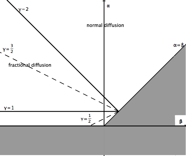
Refer to caption

Figure 1: Summary of the main results

We now turn to the proofs of Theorems 3.2 and 3.4, presented respectively in Sections 4 and 5. Concerning Theorem 3.6 we shall not write a full proof since it just follows from the proof of [7, Theorem 1] by replacing the proof of the auxiliary result in [7, Proposition 1] by Lemma 4.1 below.

4 Proof of Theorem 3.2

The general idea of the proof is the same as that of Theorem 1.1 (see Section 2). The main difference is in the derivation of formulation (19): It is no longer possible to work with the density ρε\rho^{\varepsilon} directly, and we use K⁡(fε)K(f^{\varepsilon}) instead leading to the corresponding formulation (39). This leads to another difficulty, since (39) involves an additional term which we have to show is of smaller order. Finally, we will see that the computation of the asymptotic symbol is a little bit more complicated than in Section 2 because of the collision frequency being velocity dependent, and because of the presence of the slowly varying function ℓ\ell in FF (this is the object of Proposition 4.5, in which we see appearing the importance of the different time scale that takes into account ℓ\ell and β\beta).

Throughout this section (and the next one), we denote

φ⁡(ε):=ℓ⁡(ε−11−β).\varphi(\varepsilon):=\ell(\varepsilon^{-\frac{1}{1-\beta}}).

4.1 A priori estimates

The next lemma summarizes the key properties of the collision operator LL:

Lemma 4.1.

The operator 1ν​L\frac{1}{\nu}L is bounded in L2​(ν​F−1)L^{2}(\nu F^{-1}) and satisfies:

∫ℝNL(f)fFdv≤−12​M∫ℝN|f−⟨f⟩F|2νFdv for all f∈L2(νF−1)\int_{\mathbb{R}^{N}}L(f)\frac{f}{F}\,dv\leq-\frac{1}{2M}\int_{\mathbb{R}^{N}}|f-\langle f\rangle F|^{2}\frac{\nu}{F}\,dv\hskip 10.00002pt\mbox{ for all }f\in L^{2}(\nu F^{-1}) (34)

where ⟨f⟩=∫ℝNf⁡(v)​𝑑v\langle f\rangle=\int_{\mathbb{R}^{N}}f(v)\,dv and MM is defined in (27).

Proof of Lemma 4.1. We adapt the proof of [7, Proposition 1 & 2].

To show that 1ν​L\frac{1}{\nu}L is bounded in L2​(ν​F−1)L^{2}(\nu F^{-1}), we obviously only have to check that 1ν​K\frac{1}{\nu}K is bounded. Using Cauchy-Schwartz inequality and the fact that K⁡(F)=ν​FK(F)=\nu F, we get:

‖1ν​K​(f)‖Lν​F−122\displaystyle\left\|\frac{1}{\nu}K(f)\right\|^{2}_{L^{2}_{\nu F^{-1}}} =\displaystyle= ∫K​(f)2ν​F​𝑑v\displaystyle\int\frac{K(f)^{2}}{\nu F}\,dv
≤\displaystyle\leq ∫1ν⁡(v)​F​(v)​∫σ⁡(v,v′)​F​(v′)​d​v′​∫σ⁡(v,v′)​f​(v′)2F⁡(v′)​d​v′​𝑑v\displaystyle\int\frac{1}{\nu(v)F(v)}\int\sigma(v,v^{\prime})F(v^{\prime})dv^{\prime}\int\sigma(v,v^{\prime})\frac{f(v^{\prime})^{2}}{F(v^{\prime})}\,dv^{\prime}\,dv
≤\displaystyle\leq ∫1ν⁡(v)​F​(v)​ν​(v)​F​(v)​∫σ⁡(v,v′)​f​(v′)2F⁡(v′)​d​v′​𝑑v\displaystyle\int\frac{1}{\nu(v)F(v)}\nu(v)F(v)\int\sigma(v,v^{\prime})\frac{f(v^{\prime})^{2}}{F(v^{\prime})}\,dv^{\prime}\,dv
≤\displaystyle\leq ∫∫⁡σ⁡(v,v′)​f​(v′)2F⁡(v′)​d​v′​𝑑v\displaystyle\int\int\sigma(v,v^{\prime})\frac{f(v^{\prime})^{2}}{F(v^{\prime})}\,dv^{\prime}\,dv
≤\displaystyle\leq ∫ν⁡(v′)​f​(v′)2F⁡(v′)​d​v′=‖f‖L2​(ν​F−1)2.\displaystyle\int\nu(v^{\prime})\frac{f(v^{\prime})^{2}}{F(v^{\prime})}\,dv^{\prime}=\|f\|^{2}_{L^{2}(\nu F^{-1})}.

In order to prove (34), we write

∫ℝNL⁡(f)​fF​𝑑v\displaystyle\int_{\mathbb{R}^{N}}L(f)\frac{f}{F}\,dv =\displaystyle= ∫ℝN∫ℝNσ⁡(v,v′)​f′​fF​𝑑v​d​v′−∫ℝNν⁡(v)​f2F​𝑑v\displaystyle\int_{\mathbb{R}^{N}}\int_{\mathbb{R}^{N}}\sigma(v,v^{\prime})f^{\prime}\frac{f}{F}\,dv\,dv^{\prime}-\int_{\mathbb{R}^{N}}\nu(v)\frac{f^{2}}{F}\,dv
=\displaystyle= ∫ℝN∫ℝNσ⁡(v,v′)​F′​f′F′​fF​𝑑v​d​v′−∫ℝNν⁡(v)​f2F​𝑑v.\displaystyle\int_{\mathbb{R}^{N}}\int_{\mathbb{R}^{N}}\sigma(v,v^{\prime})F^{\prime}\frac{f^{\prime}}{F^{\prime}}\frac{f}{F}\,dv\,dv^{\prime}-\int_{\mathbb{R}^{N}}\nu(v)\frac{f^{2}}{F}\,dv.

Next, we note that the second term in the right hand side can be rewritten

∫ℝNν⁡(v)​f2F​𝑑v\displaystyle\int_{\mathbb{R}^{N}}\nu(v)\frac{f^{2}}{F}\,dv =\displaystyle= ∫ℝN∫ℝNσ⁡(v′,v)​F​f2F2​𝑑v​d​v′\displaystyle\int_{\mathbb{R}^{N}}\int_{\mathbb{R}^{N}}\sigma(v^{\prime},v)F\frac{f^{2}}{F^{2}}\,dv\,dv^{\prime}
=\displaystyle= ∫ℝN∫ℝNσ⁡(v,v′)​F′​f′2F′2​𝑑v​𝑑v,\displaystyle\int_{\mathbb{R}^{N}}\int_{\mathbb{R}^{N}}\sigma(v,v^{\prime})F^{\prime}\frac{f^{\prime 2}}{F^{\prime 2}}\,dv\,dv,

as well as (using the fact that ν​F=K⁡(F)\nu F=K(F))

∫ℝNν⁡(v)​f2F​𝑑v\displaystyle\int_{\mathbb{R}^{N}}\nu(v)\frac{f^{2}}{F}\,dv =\displaystyle= ∫ℝNK⁡(F)​f2F2​𝑑v\displaystyle\int_{\mathbb{R}^{N}}K(F)\frac{f^{2}}{F^{2}}\,dv
=\displaystyle= ∫ℝN∫ℝNσ⁡(v,v′)​F′​f2F2​𝑑v​𝑑v.\displaystyle\int_{\mathbb{R}^{N}}\int_{\mathbb{R}^{N}}\sigma(v,v^{\prime})F^{\prime}\frac{f^{2}}{F^{2}}\,dv\,dv.

We deduce

∫ℝNL⁡(f)​fF​𝑑v\displaystyle\int_{\mathbb{R}^{N}}L(f)\frac{f}{F}\,dv =\displaystyle= −12∫ℝN∫ℝNσ(v,v′)F′[f′F′−fF]2dvdv′.\displaystyle-\frac{1}{2}\int_{\mathbb{R}^{N}}\int_{\mathbb{R}^{N}}\sigma(v,v^{\prime})F^{\prime}\left[\frac{f^{\prime}}{F^{\prime}}-\frac{f}{F}\right]^{2}\,dv\,dv^{\prime}. (35)

Integrating (in the v′v^{\prime} variable) the identity

f​F′−f′​F=(fF−f′F′)​F​F′f\,F^{\prime}-f^{\prime}\,F=\left(\frac{f}{F}-\frac{f^{\prime}}{F^{\prime}}\right)\,F\,F^{\prime}

we get

g=∫ℝN(fF−f′F′)​F​F′​d​v′g=\int_{\mathbb{R}^{N}}\left(\frac{f}{F}-\frac{f^{\prime}}{F^{\prime}}\right)\,F\,F^{\prime}\,dv^{\prime}

where g=f−⟨f⟩​Fg=f-\langle f\rangle F. The Cauchy-Schwarz inequality implies

g2≤(∫ℝN(fF−f′F′)2​σ​F′​d​v′)​(∫ℝNF2σ​F′​d​v′),g^{2}\leq\left(\int_{\mathbb{R}^{N}}\left(\frac{f}{F}-\frac{f^{\prime}}{F^{\prime}}\right)^{2}\,\sigma\,F^{\prime}\,dv^{\prime}\right)\ \left(\int_{\mathbb{R}^{N}}{F^{2}\over\sigma}\,F^{\prime}\,dv^{\prime}\right),

so that

∫ℝNÊ​g2F​ν​𝑑v≤(supv∈ℝNν​∫ℝNFσ​F′​d​v′)​(∫ℝN∫ℝN(fF−f′F′)2​σ​F′​d​v′​𝑑v).\int_{\mathbb{R}^{N}}Ê{g^{2}\over F}\,\nu\,dv\leq\left(\sup_{v\in\mathbb{R}^{N}}\nu\int_{\mathbb{R}^{N}}{F\over\sigma}\,F^{\prime}\,dv^{\prime}\right)\,\left(\int_{\mathbb{R}^{N}}\,\int_{\mathbb{R}^{N}}\left(\frac{f}{F}-\frac{f^{\prime}}{F^{\prime}}\right)^{2}\,\sigma\,F^{\prime}\,dv^{\prime}\,dv\right). (36)

Gathering (27), (35) and (36) we obtain (34).       

Using Lemma 4.1, we can prove the following estimate on fεf^{\varepsilon}:

Lemma 4.2.

The solution fεf^{\varepsilon} of (3) is bounded in L∞​(0,∞,L2​(F−1))L^{\infty}(0,\infty;L^{2}(F^{-1})) uniformly with respect to ε\varepsilon. Furthermore, it satisfies:

fε=ρε​F​(v)+gε,f^{\varepsilon}=\rho^{\varepsilon}F(v)+g^{\varepsilon},

where the density ρε=∫ℝNfε​𝑑v\rho^{\varepsilon}=\int_{\mathbb{R}^{N}}f^{\varepsilon}\,dv and the function gεg^{\varepsilon} are such that

‖ρε‖L∞​(0,∞,L2)≤‖f0‖L2​(F−1)\|\rho^{\varepsilon}\|_{L^{\infty}(0,\infty,L^{2})}\leq\|f_{0}\|_{L^{2}(F^{-1})} (37)

and

‖gε‖L2​(0,∞,L2​(ν​F−1))≤C​‖f0‖L2​(F−1)​θ​(ε)1/2.\|g^{\varepsilon}\|_{L^{2}(0,\infty;L^{2}(\nu F^{-1}))}\leq C\,\|f_{0}\|_{L^{2}(F^{-1})}\,\theta(\varepsilon)^{1/2}. (38)

In particular ρε\rho^{\varepsilon} converges L∞​(0,T,L2)L^{\infty}(0,T;L^{2})-weak to ρ\rho, and fεf^{\varepsilon} converges L∞​(0,T,L2​(F−1))L^{\infty}(0,T;L^{2}(F^{-1}))-weak to f=ρ⁡(t,x)​F​(v)f=\rho(t,x)F(v).

Proof of Lemma 4.2. Multiplying (3) by fε/Ff^{\varepsilon}/F, we get:

12​dd​t​∫ℝ2​N|fε|2​1F​𝑑x​𝑑v\displaystyle\frac{1}{2}\,\frac{d}{dt}\int_{\mathbb{R}^{2N}}|f^{\varepsilon}|^{2}\frac{1}{F}\,dx\,dv =\displaystyle= 1θ⁡(ε)​∫ℝ2​NL⁡(fε)​fεF\displaystyle\frac{1}{\theta(\varepsilon)}\,\int_{\mathbb{R}^{2N}}L(f^{\varepsilon})\frac{f^{\varepsilon}}{F}
≤\displaystyle\leq −12​M​θ​(ε)∫ℝ2​N|fε−ρεF|2νFdxdv\displaystyle-\frac{1}{2M\theta(\varepsilon)}\,\int_{\mathbb{R}^{2N}}|f^{\varepsilon}-\rho^{\varepsilon}F|^{2}\frac{\nu}{F}\,dx\,dv

which gives:

12​∫ℝ2​N|fε​(t,x,v)|2​1F​𝑑x​𝑑v+12​M​θ​(ε)​∫0t∫ℝ2​N|fε−ρε​F|2​νF​𝑑x​𝑑v​𝑑s\displaystyle\frac{1}{2}\,\int_{\mathbb{R}^{2N}}|f^{\varepsilon}(t,x,v)|^{2}\frac{1}{F}\,dx\,dv+\frac{1}{2M\,\theta(\varepsilon)}\,\int_{0}^{t}\int_{\mathbb{R}^{2N}}|f^{\varepsilon}-\rho^{\varepsilon}F|^{2}\frac{\nu}{F}\,dx\,dv\,ds
≤12​∫ℝ2​N|f0​(x,v)|2​1F​𝑑x​𝑑v.\displaystyle\hskip 20.00003pt\hskip 20.00003pt\hskip 20.00003pt\hskip 20.00003pt\hskip 20.00003pt\hskip 20.00003pt\hskip 20.00003pt\hskip 20.00003pt\leq\frac{1}{2}\,\int_{\mathbb{R}^{2N}}|f_{0}(x,v)|^{2}\frac{1}{F}\,dx\,dv.

This inequality shows that fεf^{\varepsilon} is bounded in L∞​(0,∞,L2​(F−1))L^{\infty}(0,\infty,L^{2}(F^{-1})). Furthermore, denoting gε=fε−ρε​Fg^{\varepsilon}=f^{\varepsilon}-\rho^{\varepsilon}F we also get

∫0t∫ℝ2​N|gε|2​νF​𝑑x​𝑑v​𝑑s≤C​‖f0‖L2​(F−1)​θ​(ε).\int_{0}^{t}\int_{\mathbb{R}^{2N}}|g^{\varepsilon}|^{2}\frac{\nu}{F}\,dx\,dv\,ds\leq C\,\|f_{0}\|_{L^{2}(F^{-1})}\,\theta(\varepsilon).

Finally, Cauchy-Schwarz inequality implies:

∫ℝN|ρε|2​𝑑x\displaystyle\int_{\mathbb{R}^{N}}|\rho^{\varepsilon}|^{2}\,dx =\displaystyle= ∫ℝN|∫ℝNfε​𝑑v|2​𝑑x\displaystyle\int_{\mathbb{R}^{N}}\left|\int_{\mathbb{R}^{N}}f^{\varepsilon}\,dv\right|^{2}\,dx
≤\displaystyle\leq ∫ℝ2​N|fε|2​1F​𝑑v​∫ℝNF​𝑑v​𝑑x=∫ℝ2​N|fε|2​1F​𝑑v​𝑑x.\displaystyle\int_{\mathbb{R}^{2N}}|f^{\varepsilon}|^{2}\frac{1}{F}\,dv\int_{\mathbb{R}^{N}}F\,dv\,dx=\int_{\mathbb{R}^{2N}}|f^{\varepsilon}|^{2}\frac{1}{F}\,dv\,dx.


4.2 Another formulation of the rescaled equation

Proceeding as in Section 2, we denote by fε^​(p,k,v)\widehat{f^{\varepsilon}}(p,k,v) the Laplace-Fourier transform of fε​(t,x,v)f^{\varepsilon}(t,x,v) with respect to tt and xx, defined by

fε^(p,k,v)=∫ℝN∫0∞e−p​te−ik⋅xfε(t,x,v)dtdx.\widehat{f^{\varepsilon}}(p,k,v)=\int_{\mathbb{R}^{N}}\int_{0}^{\infty}e^{-pt}e^{-ik\cdot x}f^{\varepsilon}(t,x,v)\,dt\,dx.

We define ρε^​(p,k)\widehat{\rho^{\varepsilon}}(p,k) and gε^​(p,k,v)\widehat{g^{\varepsilon}}(p,k,v) similarly, and we denote by f0^​(k,v)\widehat{f_{0}}(k,v) the Fourier transform of f0f_{0} with respect to xx.

Now, taking the Laplace-Fourier transform in (3), it is readily seen that fε^\widehat{f^{\varepsilon}} satisfies

θ⁡(ε)​p​fε^−θ⁡(ε)​f0^+i​v⋅k​fε^=K⁡(fε^)−ν​fε^,\theta(\varepsilon)\,p\,\widehat{f^{\varepsilon}}-\theta(\varepsilon)\,\widehat{f_{0}}+i\,v\cdot k\,\widehat{f^{\varepsilon}}=K(\widehat{f^{\varepsilon}})-\nu\,\widehat{f^{\varepsilon}},

which easily yields

fε^​(v)=θ⁡(ε)ν⁡(v)+θ⁡(ε)​p+ε​i​v⋅k​f0^+1ν⁡(v)+θ⁡(ε)​p+ε​i​v⋅k​K​(fε^).\widehat{f^{\varepsilon}}(v)=\frac{\theta(\varepsilon)}{\nu(v)+\theta(\varepsilon)p+\varepsilon iv\cdot k}\widehat{f_{0}}+\frac{1}{\nu(v)+\theta(\varepsilon)p+\varepsilon iv\cdot k}K(\widehat{f^{\varepsilon}}).

Multiplying this equality by σ⁡(w,v)\sigma(w,v) and integrating with respect to vv, we obtain

K​(fε^)​(w)\displaystyle K(\widehat{f^{\varepsilon}})(w) =\displaystyle= ∫ℝNθ⁡(ε)​σ​(w,v)ν⁡(v)+θ⁡(ε)​p+ε​i​v⋅k​f0^​(v)​𝑑v\displaystyle\int_{\mathbb{R}^{N}}\frac{\theta(\varepsilon)\sigma(w,v)}{\nu(v)+\theta(\varepsilon)p+\varepsilon iv\cdot k}\,\widehat{f_{0}}(v)\,dv
+∫ℝNσ⁡(w,v)(ν⁡(v)+θ⁡(ε)​p+ε​i​v⋅k)K(fε^)(v)dv.\displaystyle+\int_{\mathbb{R}^{N}}\frac{\sigma(w,v)}{(\nu(v)+\theta(\varepsilon)p+\varepsilon iv\cdot k)}\,K(\widehat{f^{\varepsilon}})(v)\,dv.

Finally, integrating with respect to ww, we get:

∫ℝNK​(fε^)​(v)​𝑑v\displaystyle\int_{\mathbb{R}^{N}}K(\widehat{f^{\varepsilon}})(v)\,dv =\displaystyle= ∫ℝNθ⁡(ε)​ν​(v)ν⁡(v)+θ⁡(ε)​p+ε​i​v⋅k​f0^​(v)​𝑑v\displaystyle\int_{\mathbb{R}^{N}}\frac{\theta(\varepsilon)\nu(v)}{\nu(v)+\theta(\varepsilon)p+\varepsilon iv\cdot k}\,\widehat{f_{0}}(v)\,dv
+∫ℝNν⁡(v)ν⁡(v)+θ⁡(ε)​p+ε​i​v⋅kK(fε^)(v)dv,\displaystyle+\int_{\mathbb{R}^{N}}\frac{\nu(v)}{\nu(v)+\theta(\varepsilon)p+\varepsilon iv\cdot k}\,K(\widehat{f^{\varepsilon}})(v)\,dv,

and thus

0\displaystyle 0 =\displaystyle= ∫ℝNν⁡(v)ν⁡(v)+θ⁡(ε)​p+ε​i​v⋅k​f0^​(v)​𝑑v\displaystyle\int_{\mathbb{R}^{N}}\frac{\nu(v)}{\nu(v)+\theta(\varepsilon)p+\varepsilon iv\cdot k}\,\widehat{f_{0}}(v)\,dv
+1θ⁡(ε)​(∫ℝN[ν⁡(v)ν⁡(v)+θ⁡(ε)​p+ε​i​v⋅k−1]​K​(fε^)​(v)​𝑑v).\displaystyle+\frac{1}{\theta(\varepsilon)}\,\left(\int_{\mathbb{R}^{N}}\left[\frac{\nu(v)}{\nu(v)+\theta(\varepsilon)p+\varepsilon iv\cdot k}-1\right]\,K(\widehat{f^{\varepsilon}})(v)\,dv\right).

Next, using Lemma 4.2, we write

fε^=ρε^​F+gε^\widehat{f^{\varepsilon}}=\widehat{\rho^{\varepsilon}}F+\widehat{g^{\varepsilon}}

which leads to (using the fact that K⁡(F)=ν​FK(F)=\nu F):

K⁡(fε^)=ρε^​ν​F+K⁡(gε^).K(\widehat{f^{\varepsilon}})=\widehat{\rho^{\varepsilon}}\nu F+K(\widehat{g^{\varepsilon}}).

We deduce:

0\displaystyle\!\!\!\!\!0 =\displaystyle= ∫ℝNν⁡(v)ν⁡(v)+θ⁡(ε)​p+ε​i​v⋅k​f0^​𝑑v\displaystyle\int_{\mathbb{R}^{N}}\frac{\nu(v)}{\nu(v)+\theta(\varepsilon)p+\varepsilon iv\cdot k}\,\widehat{f_{0}}\,dv (39)
+1θ⁡(ε)​(∫ℝN[ν⁡(v)ν⁡(v)+θ⁡(ε)​p+ε​i​v⋅k−1]​ν​F​𝑑v)​ρε^\displaystyle+\frac{1}{\theta(\varepsilon)}\,\left(\int_{\mathbb{R}^{N}}\left[\frac{\nu(v)}{\nu(v)+\theta(\varepsilon)p+\varepsilon iv\cdot k}-1\right]\,\nu F\,dv\right)\,\widehat{\rho^{\varepsilon}}
+1θ⁡(ε)​(∫ℝN[ν⁡(v)ν⁡(v)+θ⁡(ε)​p+ε​i​v⋅k−1]​K​(gε^)​𝑑v).\displaystyle+\frac{1}{\theta(\varepsilon)}\,\left(\int_{\mathbb{R}^{N}}\left[\frac{\nu(v)}{\nu(v)+\theta(\varepsilon)p+\varepsilon iv\cdot k}-1\right]\,K(\widehat{g^{\varepsilon}})\,dv\right).

The rest of the proof consists in passing to the limit ε→0\varepsilon\rightarrow 0 in (39).

In the next two subsections, we shall show that the last term vanishes in Lemma 4.5 and we study in Lemma 4.3 the limit of the second term

aε​(p,k):=1θ⁡(ε)​(∫ℝN[ν⁡(v)ν⁡(v)+θ⁡(ε)​p+ε​i​v⋅k−1]​ν​F​𝑑v)a^{\varepsilon}(p,k):=\frac{1}{\theta(\varepsilon)}\,\left(\int_{\mathbb{R}^{N}}\left[\frac{\nu(v)}{\nu(v)+\theta(\varepsilon)\,p+\varepsilon\,i\,v\cdot k}-1\right]\,\nu\,F\,dv\right)

as ε\varepsilon goes to zero. This limit will provide the Fourier-Laplace symbol of the asymptotic equation, and is therefore the cornerstone of the proof.

Let us prove that the first term converges to ρ^0\widehat{\rho}_{0}

∫ℝNν⁡(v)ν+θ⁡(ε)​p+ε​i​v⋅k​f^0​𝑑v⟶ρ0,for almost all ​k∈ℝN,p∈ℝ+\int_{\mathbb{R}^{N}}\frac{\nu(v)}{\nu+\theta(\varepsilon)\,p+\varepsilon\,i\,v\cdot k}\widehat{f}_{0}\,dv\longrightarrow\rho_{0},\hskip 20.00003pt\mbox{for almost all }k\in\mathbb{R}^{N},\,p\in\mathbb{R}_{+} (40)

The assumption f0∈L2​(F−1)f_{0}\in L^{2}(F^{-1}) implies in particular that f0∈Lx2​(Lv1)f_{0}\in L^{2}_{x}(L^{1}_{v}). Hence its the Fourier transform f^0\widehat{f}_{0} also belongs to Lk2​(Lv1)L^{2}_{k}(L^{1}_{v}) by Parseval equality, which means that f^0\widehat{f}_{0} is integrable in vv for almost all kk. Together with (41), this allows to apply the Lebesgue dominated convergence theorem, which yields, for almost every kk,

∫ℝNν⁡(v)ν+θ⁡(ε)​p+ε​i​v⋅k​f^0​𝑑v⟶∫ℝNf^0​𝑑v=ρ^0\int_{\mathbb{R}^{N}}\frac{\nu(v)}{\nu+\theta(\varepsilon)\,p+\varepsilon\,i\,v\cdot k}\widehat{f}_{0}\,dv\longrightarrow\int_{\mathbb{R}^{N}}\widehat{f}_{0}\,dv=\widehat{\rho}_{0}

which proves (40).

4.3 Passing to the limit in aεa^{\varepsilon}

The main goal of this section is the proof of the following proposition:

Lemma 4.3.

Recall that γ<2\gamma<2 and θ⁡(ε)=εγ​φ​(ε)\theta(\varepsilon)=\varepsilon^{\gamma}\varphi(\varepsilon), and let

aε​(p,k):=1θ⁡(ε)​∫ℝN[ν⁡(v)ν+θ⁡(ε)​p+ε​i​v⋅k−1]​ν​(v)​F​(v)​𝑑v.a^{\varepsilon}(p,k):=\frac{1}{\theta(\varepsilon)}\int_{\mathbb{R}^{N}}\left[\frac{\nu(v)}{\nu+\theta(\varepsilon)\,p+\varepsilon\,iv\cdot k}-1\right]\nu(v)F(v)\,dv.

Then

aε​(p,k)⟶−p−κ​|k|γa^{\varepsilon}(p,k)\longrightarrow-p-\kappa|k|^{\gamma}

when ε\varepsilon goes to zero, locally uniformly with respect to p≥0p\geq 0 and k∈ℝNk\in\mathbb{R}^{N}, with κ\kappa given by (31). Furthermore, aεa^{\varepsilon} is locally bounded in [0,∞]×ℝN[0,\infty]\times\mathbb{R}^{N} uniformly w.r.t. ε\varepsilon: There exists a constant CC such that

|aε​(p,k)|≤|p|+C⁡(1+|k|2).|a^{\varepsilon}(p,k)|\leq|p|+C(1+|k|^{2}).

Proof of Lemma 4.3. Observing that

|νν+θ⁡(ε)​p+ε​i​v⋅k−1|≤2,\displaystyle\left|\frac{\nu}{\nu+\theta(\varepsilon)p+\varepsilon iv\cdot k}-1\right|\leq 2, (41)

we see that aεa^{\varepsilon} is well defined for any ε>0\varepsilon>0. Next, we write

1−νν+θ⁡(ε)​p+ε​i​v⋅k\displaystyle 1-\frac{\nu}{\nu+\theta(\varepsilon)p+\varepsilon iv\cdot k} =\displaystyle= ν+θ⁡(ε)​p(ν+θ⁡(ε)​p)2+(ε​v⋅k)2​θ​(ε)​p\displaystyle\frac{\nu+\theta(\varepsilon)p}{(\nu+\theta(\varepsilon)p)^{2}+(\varepsilon v\cdot k)^{2}}\,\theta(\varepsilon)p (42)
+ε2​(v⋅k)2(ν+θ⁡(ε)​p)2+(ε​v⋅k)2\displaystyle+\,\,\,\frac{\varepsilon^{2}(v\cdot k)^{2}}{(\nu+\theta(\varepsilon)p)^{2}+(\varepsilon v\cdot k)^{2}}
+ε​ν​i​v⋅k(ν+θ⁡(ε)​p)2+(ε​v⋅k)2.\displaystyle+\,\,\,\frac{\varepsilon\nu iv\cdot k}{(\nu+\theta(\varepsilon)p)^{2}+(\varepsilon v\cdot k)^{2}}.

Using the fact that F⁡(−v)=F⁡(v)F(-v)=F(v) and ν⁡(−v)=ν⁡(v)\nu(-v)=\nu(v), we deduce

aε​(p,k)\displaystyle a^{\varepsilon}(p,k) =\displaystyle= −p∫ℝNν⁡(v)+θ⁡(ε)​p(ν⁡(v)+θ⁡(ε)​p)2+ε2​(v⋅k)2ν(v)F(v)dv\displaystyle-p\int_{\mathbb{R}^{N}}\frac{\nu(v)+\theta(\varepsilon)p}{(\nu(v)+\theta(\varepsilon)p)^{2}+\varepsilon^{2}(v\cdot k)^{2}}\nu(v)F(v)\,dv (43)
−1θ⁡(ε)∫ℝN(ε​v⋅k)2(ν⁡(v)+θ⁡(ε)​p)2+(ε​v⋅k)2ν(v)F(v)dv.\displaystyle-\frac{1}{\theta(\varepsilon)}\int_{\mathbb{R}^{N}}\frac{(\varepsilon v\cdot k)^{2}}{(\nu(v)+\theta(\varepsilon)p)^{2}+(\varepsilon v\cdot k)^{2}}\nu(v)F(v)\,dv.

The dominated convergence theorem immediately implies that the first term in the right hand side converges to −p∫ℝNF(v)dv=−p-p\int_{\mathbb{R}^{N}}F(v)\,dv=-p as ε\varepsilon goes to zero. Furthermore, that term is clearly bounded (in absolute value) by |p||p|. So it only remains to show that (and here we recall that θ⁡(ε):=εγ​φ​(ε)\theta(\varepsilon):=\varepsilon^{\gamma}\varphi(\varepsilon))

dε​(p,k):=1εγ​φ​(ε)​∫ℝN(ε​v⋅k)2(ν+εγ​φ​(ε)​p)2+(ε​v⋅k)2​ν​F​𝑑vd^{\varepsilon}(p,k):=\frac{1}{\varepsilon^{\gamma}\varphi(\varepsilon)}\int_{\mathbb{R}^{N}}\frac{(\varepsilon\,v\cdot k)^{2}}{(\nu+\varepsilon^{\gamma}\varphi(\varepsilon)p)^{2}+(\varepsilon v\cdot k)^{2}}\nu F\,dv

converges to κ​|k|γ\kappa|k|^{\gamma} and is locally bounded when ε\varepsilon goes to zero.

For some M>0M>0, we write

dε​(p,k)=d1ε​(p,k)+d2ε​(p,k)d^{\varepsilon}(p,k)=d^{\varepsilon}_{1}(p,k)+d^{\varepsilon}_{2}(p,k)

where

d1ε​(p,k)\displaystyle d^{\varepsilon}_{1}(p,k) =\displaystyle= 1εγ​φ​(ε)​∫|v|≤M(ε​v⋅k)2(ν⁡(v)+εγ​φ​(ε)​p)2+(ε​v⋅k)2​ν​(v)​F​(v)​𝑑v\displaystyle\frac{1}{\varepsilon^{\gamma}\varphi(\varepsilon)}\int_{|v|\leq M}\frac{(\varepsilon v\cdot k)^{2}}{(\nu(v)+\varepsilon^{\gamma}\varphi(\varepsilon)p)^{2}+(\varepsilon v\cdot k)^{2}}\nu(v)F(v)\,dv
≤\displaystyle\leq ε2−γ​φ​(ε)−1​∫|v|≤Mν​(v)−1​|v⋅k|2​F​(v)​𝑑v\displaystyle\varepsilon^{2-\gamma}\varphi(\varepsilon)^{-1}\int_{|v|\leq M}\nu(v)^{-1}|v\cdot k|^{2}F(v)\,dv
≤\displaystyle\leq |k|2​ε2−γ​φ​(ε)−1​∫|v|≤M|v|2​ν​(v)−1​F​(v)​𝑑v\displaystyle|k|^{2}\varepsilon^{2-\gamma}\varphi(\varepsilon)^{-1}\int_{|v|\leq M}|v|^{2}\,\nu(v)^{-1}\,F(v)\,dv
≤\displaystyle\leq C​|k|2​ε2−γ​φ​(ε)−1\displaystyle C\,|k|^{2}\,\varepsilon^{2-\gamma}\,\varphi(\varepsilon)^{-1}

(using the assumption (A2) that |v|2​ν​(v)−1​F|v|^{2}\,\nu(v)^{-1}\,F is locally integrable) and

d2ε​(p,k)=1εγ​φ​(ε)​∫|v|≥M(ε​v⋅k)2(ν⁡(v)+εγ​φ​(ε)​p)2+(ε​v⋅k)2​ν​(v)​F​(v)​𝑑v.d_{2}^{\varepsilon}(p,k)=\frac{1}{\varepsilon^{\gamma}\,\varphi(\varepsilon)}\int_{|v|\geq M}\frac{(\varepsilon\,v\cdot k)^{2}}{(\nu(v)+\varepsilon^{\gamma}\,\varphi(\varepsilon)p)^{2}+(\varepsilon\,v\cdot k)^{2}}\nu(v)F(v)\,dv.

It is readily seen (using (46) and the fact that γ<2\gamma<2) that

d1ε​(p,k)⟶0​ as ​ε→0.d_{1}^{\varepsilon}(p,k)\longrightarrow 0\mbox{ as }\varepsilon\rightarrow 0.

Furthermore, d1εd_{1}^{\varepsilon} is bounded, for ε\varepsilon small enough by C​|k|2C|k|^{2}. So we only need to evaluate the limit of d2ε​(p,k)d_{2}^{\varepsilon}(p,k). For that purpose, we first rewrite d2εd_{2}^{\varepsilon} as follows:

d2ε​(p,k)=1εγ​φ​(ε)​∫|v|≥M(|v|−β​ε​v⋅k)2(ν~​(v)+|v|−β​εγ​φ​(ε)​p)2+(|v|−β​ε​v⋅k)2​ν~​(v)​F~0​(v)​ℓ​(|v|)|v|N+α−β​𝑑v.d_{2}^{\varepsilon}(p,k)=\frac{1}{\varepsilon^{\gamma}\varphi(\varepsilon)}\int_{|v|\geq M}\frac{(|v|^{-\beta}\,\varepsilon\,v\cdot k)^{2}}{(\widetilde{\nu}(v)+|v|^{-\beta}\,\varepsilon^{\gamma}\,\varphi(\varepsilon)\,p)^{2}+(|v|^{-\beta}\,\varepsilon\,v\cdot k)^{2}}\frac{\widetilde{\nu}(v)\,\widetilde{F}_{0}(v)\,\ell(|v|)}{|v|^{N+\alpha-\beta}}\,dv.

where

ν~​(v)=|v|−β​ν​(v) and F~0​(v)=|v|N+α​F0​(v).\widetilde{\nu}(v)=|v|^{-\beta}\,\nu(v)\hskip 10.00002pt\mbox{ and }\hskip 10.00002pt\widetilde{F}_{0}(v)=|v|^{N+\alpha}\,F_{0}(v).

Note that Assumptions (B1-B2-B3) (see also (28)) imply that ν~\widetilde{\nu} and F~0\widetilde{F}_{0} are uniformly bounded from above and below for |v|≥M|v|\geq M for a suitable M>0M>0, and that

lim|v|→∞ν~​(v)=ν0 and lim|v|→∞F~0​(v)=κ0.\lim_{|v|\rightarrow\infty}\widetilde{\nu}(v)=\nu_{0}\hskip 10.00002pt\mbox{ and }\hskip 10.00002pt\lim_{|v|\rightarrow\infty}\widetilde{F}_{0}(v)=\kappa_{0}. (44)

We now do the change of variable

w=ε​|k|​|v|−β​v,w=\varepsilon|k||v|^{-\beta}v,

for which we have:

|v|=|w|11−β(ε​|k|)11−β,v=w|w|−β1−β​(ε​|k|)11−β, and dv=(1−β)−1(ε​|k|)N1−β​|w|−β​N1−βdw.|v|=\frac{|w|^{\frac{1}{1-\beta}}}{(\varepsilon|k|)^{\frac{1}{1-\beta}},}\hskip 20.00003ptv=\frac{w}{|w|^{\frac{-\beta}{1-\beta}}(\varepsilon|k|)^{\frac{1}{1-\beta}}},\hskip 10.00002pt\mbox{ and }\hskip 10.00002ptdv=\frac{(1-\beta)^{-1}}{(\varepsilon|k|)^{\frac{N}{1-\beta}}|w|^{\frac{-\beta N}{1-\beta}}}\,dw.

We obtain (with e=k/|k|e=k/|k|):

d2ε​(p,k)=\displaystyle\!\!\!\!\!\!\!\!\!\!d_{2}^{\varepsilon}(p,k)=
=(1−β)−1εγ​φ​(ε)​∫|w|≥M1−β​ε​|k|(w⋅e)2(ν~ε​(w)+|w|−β1−β​(ε​|k|)β1−β​εγ​φ​(ε)​p)2+(w⋅e)2\displaystyle\!\!\!\!=\frac{(1-\beta)^{-1}}{\varepsilon^{\gamma}\varphi(\varepsilon)}\int_{|w|\geq M^{1-\beta}\varepsilon|k|}\;\;\frac{(w\cdot e)^{2}}{(\widetilde{\nu}^{\varepsilon}(w)+|w|^{\frac{{-\beta}}{1-\beta}}(\varepsilon|k|)^{\frac{\beta}{1-\beta}}\varepsilon^{\gamma}\varphi(\varepsilon)p)^{2}+(w\cdot e)^{2}}
×ν~ε​(w)​F~0ε​(w)|w|N+α−β1−β​(ε​|k|)N+α−β1−β​ℓ​(|w|11−β(ε​|k|)11−β)​(ε​|k|)−N1−β​|w|−N−β1−β​d​w.\displaystyle\hskip 20.00003pt\times\frac{\widetilde{\nu}^{\varepsilon}(w)\widetilde{F}^{\varepsilon}_{0}(w)}{|w|^{\frac{N+\alpha-\beta}{1-\beta}}}(\varepsilon|k|)^{\frac{N+\alpha-\beta}{1-\beta}}\ell\left(\frac{|w|^{\frac{1}{1-\beta}}}{(\varepsilon|k|)^{\frac{1}{1-\beta}}}\right)\,(\varepsilon|k|)^{-\frac{N}{1-\beta}}|w|^{-\frac{N-\beta}{1-\beta}}\,dw.

where

ν~ε​(w)=ν~​(w|w|−β1−β​(ε​|k|)11−β)\widetilde{\nu}^{\varepsilon}(w)=\widetilde{\nu}\left(\frac{w}{|w|^{\frac{-\beta}{1-\beta}}(\varepsilon|k|)^{\frac{1}{1-\beta}}}\right)

and

F~0ε​(w)=F~0​(w|w|−β1−β​(ε​|k|)11−β)\widetilde{F}_{0}^{\varepsilon}(w)=\widetilde{F}_{0}\left(\frac{w}{|w|^{\frac{-\beta}{1-\beta}}(\varepsilon|k|)^{\frac{1}{1-\beta}}}\right)

(we dropped the dependence in kk in ν~ε\widetilde{\nu}^{\varepsilon} and F~0ε\widetilde{F}_{0}^{\varepsilon} to keep notation simpler). The definition of γ\gamma thus gives:

d2ε​(p,k)=\displaystyle\!\!\!\!\!\!\!\!\!\!d_{2}^{\varepsilon}(p,k)=
=(1−β)−1​|k|γ​∫|w|≥M1−β​ε​|k|(w⋅e)2(ν~ε​(w)+|w|−β1−β​|k|β1−β​φ​(ε)​εα1−β​p)2+(w⋅e)2\displaystyle\!\!\!\!=(1-\beta)^{-1}|k|^{\gamma}\int_{|w|\geq M^{1-\beta}\varepsilon|k|}\frac{(w\cdot e)^{2}}{(\widetilde{\nu}^{\varepsilon}(w)+|w|^{\frac{-\beta}{1-\beta}}|k|^{\frac{\beta}{1-\beta}}\varphi(\varepsilon)\varepsilon^{\frac{\alpha}{1-\beta}}p)^{2}+(w\cdot e)^{2}}
×ν~ε​(w)​F~0ε​(w)|w|N+γ​ℓ​(|w|11−β(ε​|k|)11−β)​1φ⁡(ε)​d​w.\displaystyle\hskip 10.00002pt\times\frac{\widetilde{\nu}^{\varepsilon}(w)\widetilde{F}^{\varepsilon}_{0}(w)}{|w|^{N+\gamma}}\ell\left(\frac{|w|^{\frac{1}{1-\beta}}}{(\varepsilon|k|)^{\frac{1}{1-\beta}}}\right)\frac{1}{\varphi(\varepsilon)}\,dw. (45)

Finally, we note that for any ww and kk, we have (note that β<1\beta<1)

limε→0ν~ε​(w)=ν0\lim_{\varepsilon\rightarrow 0}\widetilde{\nu}^{\varepsilon}(w)=\nu_{0}
limε→0F~0ε​(w)=κ0\lim_{\varepsilon\rightarrow 0}\widetilde{F}_{0}^{\varepsilon}(w)=\kappa_{0}

and

limε→01φ⁡(ε)​ℓ​(|w|11−β(ε​|k|)11−β)=limε→01ℓ⁡(ε−11−β)​ℓ​(|w|11−β(ε​|k|)11−β)=1.\lim_{\varepsilon\rightarrow 0}\frac{1}{\varphi(\varepsilon)}\ell\left(\frac{|w|^{\frac{1}{1-\beta}}}{(\varepsilon|k|)^{\frac{1}{1-\beta}}}\right)=\lim_{\varepsilon\rightarrow 0}\frac{1}{\ell(\varepsilon^{-\frac{1}{1-\beta}})}\ell\left(\frac{|w|^{\frac{1}{1-\beta}}}{(\varepsilon|k|)^{\frac{1}{1-\beta}}}\right)=1.

Thus, the integrand in (45) converges pointwise to

(w⋅e)2ν02+(w⋅e)2​ν0​κ0|w|N+γ.\frac{(w\cdot e)^{2}}{\nu_{0}^{2}+(w\cdot e)^{2}}\frac{\nu_{0}\kappa_{0}}{|w|^{N+\gamma}}.

Furthermore, it is bounded by

C​(w⋅e)2ν12+(w⋅e)2​1|w|N+γ​(1+(|w||k|)δ)C\frac{(w\cdot e)^{2}}{\nu_{1}^{2}+(w\cdot e)^{2}}\frac{1}{|w|^{N+\gamma}}\left(1+\left(\frac{|w|}{|k|}\right)^{\delta}\right)

thanks to the following lemma and an appropriate choice of MM, see the following lemma (extracted from [3, Theorem 1.5.6]):

Lemma 4.4 (Potter’s Theorem).

For all δ>0\delta>0 there exists some constants C,M>0C,M>0 such that

|ℓ⁡(λ​s)ℓ⁡(s)|≤C⁡(1+|λ|δ) for all ​s≥M​ and ​λ≥M/s.\left|\frac{\ell(\lambda s)}{\ell(s)}\right|\leq C(1+|\lambda|^{\delta})\hskip 20.00003pt\mbox{ for all }s\geq M\mbox{ and }\lambda\geq M/s.

Moreover for any ζ>0\zeta>0:

sζ​ℓ​(s)⟶∞ and s−ζ​ℓ​(s)⟶0 as s→∞.s^{\zeta}\ell(s)\longrightarrow\infty\hskip 10.00002pt\mbox{ and }\hskip 10.00002pts^{-\zeta}\ell(s)\longrightarrow 0\hskip 10.00002pt\mbox{ as }\hskip 10.00002pts\rightarrow\infty. (46)

Choosing 0<δ≤γ/20<\delta\leq\gamma/2 (and thus fixing a corresponding constant MM), we deduce that

|d2ε​(p,k)|≤C​|k|γ​(1+|k|−δ)|d_{2}^{\varepsilon}(p,k)|\leq C\,|k|^{\gamma}\,(1+|k|^{-\delta})

and by Lebesgue’s dominated convergence theorem we get:

d2ε​(p,k)⟶(1−β)−1​|k|γ​∫ℝN(w⋅e)2ν02+(w⋅e)2​ν0​κ0|w|N+γ​𝑑w=κ​|k|γ,\displaystyle d_{2}^{\varepsilon}(p,k)\longrightarrow(1-\beta)^{-1}\,|k|^{\gamma}\,\int_{\mathbb{R}^{N}}\frac{(w\cdot e)^{2}}{\nu_{0}^{2}+(w\cdot e)^{2}}\frac{\nu_{0}\kappa_{0}}{|w|^{N+\gamma}}\,dw=\kappa\,|k|^{\gamma},

which concludes the proof.       

4.4 The remaining term

We will also need the following technical lemma to pass to the limit in the first and last term in (39). Note that we directly include in this lemma the limit case γ=2\gamma=2 since we shall need it this same technical lemma in this limit case for the proof of Theorem 3.4.

Lemma 4.5.

Assume (A1-A2) and (B1-B2-B3) with α>0\alpha>0, β<α\beta<\alpha and β≤2−α\beta\leq 2-\alpha.

Then

∫ℝN|ν⁡(v)ν+θ⁡(ε)​p+ε​i​v⋅k−1|​ν​(v)​F​(v)​𝑑v≤C⁡(p,k)​εmin⁡{γ/2+η; 1}\displaystyle\!\!\!\!\!\!\!\!\!\!\!\!\!\!\!\!\int_{\mathbb{R}^{N}}\left|\frac{\nu(v)}{\nu+\theta(\varepsilon)\,p+\varepsilon\,iv\cdot k}-1\right|\nu(v)F(v)\,dv\leq C(p,k)\,\varepsilon^{\min\{\gamma/2+\eta\,;\,1\}} (47)

for some η>0\eta>0, all k∈ℝN,p∈ℝ+k\in\mathbb{R}^{N},\,p\in\mathbb{R}_{+}, and C⁡(p,k)∈Ll​o​c∞​(ℝ+×ℝN)C(p,k)\in L^{\infty}_{loc}(\mathbb{R}_{+}\times\mathbb{R}^{N}).

Remarks 4.6.

Note that the assumptions of Lemma 4.5 imply that 0<γ≤20<\gamma\leq 2, and therefore γ=2\gamma=2 is included in these assumptions, except when α=1\alpha=1. In other words we exclude the case α=β=1\alpha=\beta=1 and hence when γ=2\gamma=2 we always suppose α>1\alpha>1.

Proof of Lemma 4.5.

To prove (47), we split the integral into three part parts:

∫ℝN|ν⁡(v)ν+θ⁡(ε)​p+ε​i​v⋅k−1|​ν​(v)​F​(v)​𝑑v=c+ε​(p,k)+c−ε​(p,k)\int_{\mathbb{R}^{N}}\left|\frac{\nu(v)}{\nu+\theta(\varepsilon)\,p+\varepsilon\,iv\cdot k}-1\right|\nu(v)F(v)\,dv=c_{+}^{\varepsilon}(p,k)+c_{-}^{\varepsilon}(p,k)

where

c±ε(p,k):=∫{|v|±1≤ε∓11−β}|ν⁡(v)ν+θ⁡(ε)​p+ε​i​v⋅k−1|ν(v)F(v)dvc_{\pm}^{\varepsilon}(p,k):=\int_{\left\{|v|^{\pm 1}\leq\;\varepsilon^{\frac{\mp 1}{1-\beta}}\right\}}\left|\frac{\nu(v)}{\nu+\theta(\varepsilon)\,p+\varepsilon\,iv\cdot k}-1\right|\nu(v)F(v)\,dv

(note that this splitting is well-defined since β≠1\beta\neq 1 in the assumptions).

In order to get a bound for c+εc_{+}^{\varepsilon}, we note that (42) implies:

|νν+θ⁡(ε)​p+ε​i​v⋅k−1|\displaystyle\left|\frac{\nu}{\nu+\theta(\varepsilon)p+\varepsilon\,i\,v\cdot k}-1\right| ≤\displaystyle\leq ν−1​θ​(ε)​|p|+ε2​ν−2​(v⋅k)2+ε​ν−1​|v⋅k|\displaystyle\nu^{-1}\,\theta(\varepsilon)\,|p|+\varepsilon^{2}\nu^{-2}(v\cdot k)^{2}+\varepsilon\,\nu^{-1}\,|v\cdot k|

and thus

c+ε​(p,k)\displaystyle c_{+}^{\varepsilon}(p,k) ≤\displaystyle\leq θ⁡(ε)​|p|​∫ℝNF⁡(v)​𝑑v\displaystyle\theta(\varepsilon)\,|p|\,\int_{\mathbb{R}^{N}}F(v)\,dv
+(ε|k|)2∫{|v|≤ε−11−β}|v|2ν−1(v)F(v)dv\displaystyle+(\varepsilon\,|k|)^{2}\,\int_{\left\{|v|\leq\,\varepsilon^{\frac{-1}{1-\beta}}\right\}}|v|^{2}\,\nu^{-1}(v)\,F(v)\,dv
+ε|k|∫{|v|≤ε−11−β}|v|F(v)dv.\displaystyle+\varepsilon\,|k|\,\int_{\left\{|v|\leq\;\varepsilon^{\frac{-1}{1-\beta}}\right\}}|v|\,F(v)\,dv.

We write

c+ε​(p,k)\displaystyle c_{+}^{\varepsilon}(p,k)\! ≤\displaystyle\leq θ⁡(ε)​|p|+(ε​|k|)2​c+,2ε​(p,k)+ε​|k|​c+,3ε​(p,k).\displaystyle\!\theta(\varepsilon)\,|p|+(\varepsilon\,|k|)^{2}\,c_{+,2}^{\varepsilon}(p,k)+\varepsilon\,|k|\,c_{+,3}^{\varepsilon}(p,k).

The computation of c+,2ε​(p,k)c_{+,2}^{\varepsilon}(p,k) requires the computation of the following integral:

∫{|v|≤ε−11−β}|v|2ν−1(v)F(v)dv\int_{\left\{|v|\leq\;\varepsilon^{\frac{-1}{1-\beta}}\right\}}|v|^{2}\,\nu^{-1}(v)\,F(v)\,dv

which we estimate using the assumption (A2) that |v|2​ν​(v)−1​F|v|^{2}\,\nu(v)^{-1}\,F is locally integrable, and the fact that F⁡(v)≤C1​ℓ​(v)​|v|−N−αF(v)\leq C_{1}\,\ell(v)\,|v|^{-N-\alpha} and ν⁡(v)≥C2​|v|β\nu(v)\geq C_{2}\,|v|^{\beta} for |v|≥M|v|\geq M. When β≠2−α\beta\neq 2-\alpha, it yields

c+,2ε≤C⁡(1+εγ−2−δ)c_{+,2}^{\varepsilon}\leq C\,\left(1+\varepsilon^{\gamma-2-\delta}\right)

for some δ\delta as small as we want, using the Potter’s lemma 4.4 to estimate ℓ\ell. In the case when β=2−α\beta=2-\alpha, it yields

c+,2ε≤C(1+Ξ(ε−1/(1−β)))c_{+,2}^{\varepsilon}\leq C\,\left(1+\Xi\left(\varepsilon^{-1/(1-\beta)}\right)\right)

with

Ξ⁡(z):=∫Mzℓ⁡(r)r​𝑑r​if​z≥M,Ξ⁡(z):=0​if​z≤M.\Xi(z):=\int_{M}^{z}\frac{\ell(r)}{r}\,dr\,\,\hbox{if}\,\,z\geq M,\hskip 10.00002pt\Xi(z):=0\,\,\hbox{if}\,\,z\leq M.

In both cases this yields, by fixing δ=γ/2\delta=\gamma/2, using the trivial estimate

z−δ​Ξ​(z)→z→+∞0z^{-\delta}\,\Xi(z)\xrightarrow[z\to+\infty]{}0

for any δ>0\delta>0, and keeping only higher order terms, we obtain the following (non optimal) bound:

(ε​|k|)2​c+,2ε​(p,k)≤C​εγ/2+η(\varepsilon\,|k|)^{2}\,c_{+,2}^{\varepsilon}(p,k)\leq C\,\varepsilon^{\gamma/2+\eta}

for some η>0\eta>0.

Similarly we found

c+,3ε≤C(1+εγ−1−δ)ifα≠1,c+,3ε≤C(1+Ξ(ε−1/(1−β)))ifα=1c_{+,3}^{\varepsilon}\leq C\,\left(1+\varepsilon^{\gamma-1-\delta}\right)\,\,\hbox{if}\,\,\alpha\neq 1,\hskip 10.00002ptc_{+,3}^{\varepsilon}\leq C\,\left(1+\Xi\left(\varepsilon^{-1/(1-\beta)}\right)\right)\,\,\hbox{if}\,\,\alpha=1

for some δ\delta as small as we want.

Using the same arguments as before (and recalling that when α=1\alpha=1, γ=2\gamma=2 is not allowed since β<α\beta<\alpha), we get

(ε​|k|)​c+,3ε​(p,k)≤C​(ε​|k|)min⁡{γ/2+η; 1}(\varepsilon\,|k|)\,c_{+,3}^{\varepsilon}(p,k)\leq C\,(\varepsilon|k|)^{\min\{\gamma/2+\eta\;;\;1\}}

for some η>0\eta>0.

Finally, in order to get a bound on c−εc_{-}^{\varepsilon}, we do the change of variable w=ε11−β​vw=\varepsilon^{\frac{1}{1-\beta}}\,v which leads to

c−ε(p,k)≤∫{|v|≥ε−11−β}2ν(v)F(v)dv\displaystyle\!\!\!\!\!\!\!\!\!c_{-}^{\varepsilon}(p,k)\leq\int_{\left\{|v|\geq\;\varepsilon^{\frac{-1}{1-\beta}}\right\}}2\,\nu(v)F(v)\,dv
≤\displaystyle\leq 2​εα−β1−β​∫|w|≥1νε~​(w)​F~0ε​(w)|w|N+α−β​ℓ​(|w|​ε−11−β)​𝑑w\displaystyle 2\,\varepsilon^{\frac{\alpha-\beta}{1-\beta}}\int_{|w|\geq 1}\frac{\widetilde{\nu^{\varepsilon}}(w)\widetilde{F}_{0}^{\varepsilon}(w)}{|w|^{N+\alpha-\beta}}{\ell(|w|\,\varepsilon^{\frac{-1}{1-\beta}})}\,dw
≤C​εγ​φ​(ε)​∫|w|≥1|w|−N−α+β​(1+|w|δ)​𝑑w\displaystyle\!\!\!\!\!\!\leq C\,\varepsilon^{\gamma}\,\varphi(\varepsilon)\int_{|w|\geq 1}|w|^{-N-\alpha+\beta}\left(1+|w|^{\delta}\right)\,dw
≤C′​εγ​φ​(ε)\displaystyle\!\!\!\!\!\!\leq C^{\prime}\,\varepsilon^{\gamma}\,\varphi(\varepsilon)

where we used Potter’s lemma 4.4 for some δ>0\delta>0.

Collecting all the terms, and keeping only higher order terms, we find easily (47).       

Finally we show that the last term in (39) goes to zero in 𝒟′​([0,∞]×ℝN)\mathcal{D}^{\prime}([0,\infty]\times\mathbb{R}^{N}): First, we note that for any g∈L2​(ν​F−1)g\in L^{2}(\nu F^{-1}), we have by Cauchy-Schwarz inequality and assumption (27)

|K⁡(g)|\displaystyle|K(g)| ≤\displaystyle\leq ∫ℝNσ⁡(v,v′)​|g⁡(v′)|​d​v′\displaystyle\int_{\mathbb{R}^{N}}\sigma(v,v^{\prime})|g(v^{\prime})|\,dv^{\prime}
≤\displaystyle\leq (∫ℝNσ2​F′ν′​d​v′)1/2​(∫ℝN|g⁡(v′)|2F⁡(v′)​ν′​d​v′)1/2\displaystyle\left(\int_{\mathbb{R}^{N}}\sigma^{2}\,{F^{\prime}\over\nu^{\prime}}\,dv^{\prime}\right)^{1/2}\left(\int_{\mathbb{R}^{N}}\frac{|g(v^{\prime})|^{2}}{F(v^{\prime})}\,\nu^{\prime}\,dv^{\prime}\right)^{1/2}
≤\displaystyle\leq M​Ê​ν​F​‖g‖L2​(ν​F−1).\displaystyle MÊ\,\nu\,F\,\|g\|_{L^{2}(\nu F^{-1})}.

Next, using Lemma 4.5, we deduce that

|1θ⁡(ε)​∫ℝN[ν⁡(v)ν⁡(v)+θ⁡(ε)​p+ε​i​v⋅k−1]​K​(gε^)​(v)​𝑑v|\displaystyle\left|\frac{1}{\theta(\varepsilon)}\int_{\mathbb{R}^{N}}\left[\frac{\nu(v)}{\nu(v)+\theta(\varepsilon)p+\varepsilon iv\cdot k}-1\right]K(\widehat{g^{\varepsilon}})(v)\,dv\right|
≤Cθ⁡(ε)​(∫ℝN|ν⁡(v)ν⁡(v)+θ⁡(ε)​p+ε​i​v⋅k−1|​ν​(v)​F​(v)​𝑑v)​‖gε^‖L2​(ν​F−1)\displaystyle\hskip 20.00003pt\leq\frac{C}{\theta(\varepsilon)}\left(\int_{\mathbb{R}^{N}}\left|\frac{\nu(v)}{\nu(v)+\theta(\varepsilon)p+\varepsilon iv\cdot k}-1\right|\nu(v)F(v)\,dv\right)\;\|\widehat{g^{\varepsilon}}\|_{L^{2}(\nu F^{-1})}
≤C⁡(p,k)θ⁡(ε)​εγ/2+η​‖gε^‖L2​(ν​F−1).\displaystyle\hskip 20.00003pt\leq\frac{C(p,k)}{\theta(\varepsilon)}\,\varepsilon^{\gamma/2+\eta}\;\|\widehat{g^{\varepsilon}}\|_{L^{2}(\nu F^{-1})}.

Note that here since γ<2\gamma<2, one can find η>0\eta>0 such that γ/2+η<1\gamma/2+\eta<1, and therefore the estimate (47) in Lemma 4.5 yields a bound from the below of the form C​εγ/2+ηC\,\varepsilon^{\gamma/2+\eta}.

Last, recalling inequality (38), we have for any test function ϕ∈𝒟⁡((0,∞)×ℝN)\phi\in\mathcal{D}((0,\infty)\times\mathbb{R}^{N}):

|∫0∞∫ℝNϕ⁡(p,k)​1θ⁡(ε)​∫ℝN[ν⁡(v)ν⁡(v)+θ⁡(ε)​p+ε​i​v⋅k−1]​K​(gε^)​(v)​𝑑v​𝑑k​𝑑p|\displaystyle\left|\int_{0}^{\infty}\int_{\mathbb{R}^{N}}\phi(p,k)\frac{1}{\theta(\varepsilon)}\int_{\mathbb{R}^{N}}\left[\frac{\nu(v)}{\nu(v)+\theta(\varepsilon)p+\varepsilon iv\cdot k}-1\right]\,K(\widehat{g^{\varepsilon}})(v)\,dv\,dk\,dp\right|
≤C​εγ/2+ηθ⁡(ε)​(∫0∞(∫ℝNC​(p,k)2​ϕ​(p,k)2​𝑑k)1/2​𝑑p)\displaystyle\hskip 20.00003pt\leq\frac{C\,\varepsilon^{\gamma/2+\eta}}{\theta(\varepsilon)}\,\left(\int_{0}^{\infty}\left(\int_{\mathbb{R}^{N}}C(p,k)^{2}\,\phi(p,k)^{2}\,dk\,\right)^{1/2}dp\right)
×‖gε^‖L∞​((a,∞),L2​(ν​F−1))\displaystyle\hskip 20.00003pt\hskip 10.00002pt\hskip 10.00002pt\hskip 10.00002pt\times\|\widehat{g^{\varepsilon}}\|_{L^{\infty}((a,\infty);L^{2}(\nu F^{-1}))}
≤C⁡(ϕ)​εγ/2+ηθ⁡(ε)​‖gε‖L2​((0,∞),L2​(ν​F−1))\displaystyle\hskip 20.00003pt\leq\frac{C(\phi)\,\varepsilon^{\gamma/2+\eta}}{\theta(\varepsilon)}\,\|{g^{\varepsilon}}\|_{L^{2}((0,\infty);L^{2}(\nu F^{-1}))}
≤C⁡(ϕ)​εη​φ​(ε)−1\displaystyle\hskip 20.00003pt\leq C(\phi)\,\varepsilon^{\eta}\,\varphi(\varepsilon)^{-1}

which goes to zero thanks to (46) and the fact that η>0\eta>0.       

4.5 Conclusion

We now have all the tools to pass to the limit ε→0\varepsilon\rightarrow 0 in (39). The first part of Lemma 4.5 implies that the first term converges to ρ0^​(k)\widehat{\rho_{0}}(k) locally uniformly with respect to kk and pp, while the second term can be rewritten as aε​(p,k)​ρε^a^{\varepsilon}(p,k)\widehat{\rho^{\varepsilon}} which converges, using Lemma 4.3, in 𝒟′​((0,∞)×ℝN)\mathcal{D}^{\prime}((0,\infty)\times\mathbb{R}^{N}) to (−p−κ​|k|γ)​ρ^(-p-\kappa|k|^{\gamma})\widehat{\rho}.

The remaining term goes to 00 thanks the the second part of Lemma 4.5 and the preceeding subsection.

Hence we can pass to the limit in (39) and recover (21). The proof of Theorem 3.2 can then be completed as the proof of Theorem 1.1.

5 Proof of Theorem 3.4

The proof of Theorem 3.6 is very similar to the proof of Theorem 3.2. We recall the main steps for the reader’s sake.

We recall that we define the following time scale in the critical case:

θ⁡(ε)=ε2​ℓ​(ε−11−β)​ln⁡(ε−1).\theta(\varepsilon)=\varepsilon^{2}\,\ell(\varepsilon^{-\frac{1}{1-\beta}})\,\ln(\varepsilon^{-1}).

and we shall use the same notation as in the previous section:

φ⁡(ε)=ℓ⁡(ε−11−β).\varphi(\varepsilon)=\ell(\varepsilon^{-\frac{1}{1-\beta}}).

The starting point is again the equality (39). As in the previous section, we see that if we take that the first term converges to ρ0\rho_{0} when ε\varepsilon goes to zero.

Proceeding as in Section 4.4 we can also show (using Lemma 4.5 with γ=2\gamma=2) that the last term goes to zero:

|1θ⁡(ε)​∫ℝN[ν⁡(v)ν⁡(v)+θ⁡(ε)​p+ε​i​v⋅k−1]​K​(gε^)​(v)​𝑑v|\displaystyle\left|\frac{1}{\theta(\varepsilon)}\int_{\mathbb{R}^{N}}\left[\frac{\nu(v)}{\nu(v)+\theta(\varepsilon)p+\varepsilon iv\cdot k}-1\right]K(\widehat{g^{\varepsilon}})(v)\,dv\right|
≤Cθ⁡(ε)​(∫ℝN|ν⁡(v)ν⁡(v)+θ⁡(ε)​p+ε​i​v⋅k−1|​ν​(v)​F​(v)​𝑑v)​‖gε^‖L2​(ν​F−1)\displaystyle\hskip 20.00003pt\leq\frac{C}{\theta(\varepsilon)}\left(\int_{\mathbb{R}^{N}}\left|\frac{\nu(v)}{\nu(v)+\theta(\varepsilon)p+\varepsilon iv\cdot k}-1\right|\nu(v)F(v)\,dv\right)\;\|\widehat{g^{\varepsilon}}\|_{L^{2}(\nu F^{-1})}
≤C⁡(p,k)θ⁡(ε)​ε​‖gε^‖L2​(ν​F−1).\displaystyle\hskip 20.00003pt\leq\frac{C(p,k)}{\theta(\varepsilon)}\,\varepsilon\;\|\widehat{g^{\varepsilon}}\|_{L^{2}(\nu F^{-1})}.

Note that here since γ=2\gamma=2, the estimate (47) in Lemma 4.5 yields a bound from the below of the form C​εC\,\varepsilon.

Last, recalling inequality (38), we have for any test function ϕ∈𝒟⁡((0,∞)×ℝN)\phi\in\mathcal{D}((0,\infty)\times\mathbb{R}^{N}):

|∫0∞∫ℝNϕ⁡(p,k)​1θ⁡(ε)​∫ℝN[ν⁡(v)ν⁡(v)+θ⁡(ε)​p+ε​i​v⋅k−1]​K​(gε^)​(v)​𝑑v​𝑑k​𝑑p|\displaystyle\left|\int_{0}^{\infty}\int_{\mathbb{R}^{N}}\phi(p,k)\frac{1}{\theta(\varepsilon)}\int_{\mathbb{R}^{N}}\left[\frac{\nu(v)}{\nu(v)+\theta(\varepsilon)p+\varepsilon iv\cdot k}-1\right]\,K(\widehat{g^{\varepsilon}})(v)\,dv\,dk\,dp\right|
≤C​εθ⁡(ε)​(∫0∞(∫ℝNC​(p,k)2​ϕ​(p,k)2​𝑑k)1/2​𝑑p)​‖gε^‖L∞​((a,∞),L2​(ν​F−1))\displaystyle\hskip 20.00003pt\leq\frac{C\,\varepsilon}{\theta(\varepsilon)}\,\left(\int_{0}^{\infty}\left(\int_{\mathbb{R}^{N}}C(p,k)^{2}\,\phi(p,k)^{2}\,dk\,\right)^{1/2}dp\right)\,\|\widehat{g^{\varepsilon}}\|_{L^{\infty}((a,\infty);L^{2}(\nu F^{-1}))}
≤C⁡(ϕ)​εθ⁡(ε)​‖gε‖L2​((0,∞),L2​(ν​F−1))\displaystyle\hskip 20.00003pt\leq\frac{C(\phi)\,\varepsilon}{\theta(\varepsilon)}\,\|{g^{\varepsilon}}\|_{L^{2}((0,\infty);L^{2}(\nu F^{-1}))}
≤C⁡(ϕ)φ⁡(ε)​ln⁡(ε−1)\displaystyle\hskip 20.00003pt\leq\frac{C(\phi)}{\varphi(\varepsilon)\,\ln(\varepsilon^{-1})}

which goes to zero thanks to assumption (32) in Theorem 3.4: ℓ⁡(r)​ln⁡r→+∞\ell(r)\,\ln r\to+\infty as r→+∞r\to+\infty indeed immediately implies that ℓ(ε−1/(1−β))ln(ε−1)→+∞\ell(\varepsilon^{-1/(1-\beta)})\,\ln(\varepsilon^{-1})\to+\infty as ε→0\varepsilon\to 0 (recall that here 1−β=α−1>01-\beta=\alpha-1>0).

Finally, we are left with the task of determining the limit of the symbol aεa^{\varepsilon} in (43).

It has already been proved that the first term in the right hand side of (43) is bounded (uniformly in ε\varepsilon) by |p||p| and converges to −p∫ℝNF(v)dv=−p-p\int_{\mathbb{R}^{N}}F(v)\,dv=-p as ε\varepsilon goes to zero.

So it only remains to show that

dε​(p,k):=1θ⁡(ε)​∫ℝN(ε​v⋅k)2(ν+θ⁡(ε)​p)2+(ε​v⋅k)2​ν​(v)​F​(v)​𝑑vd^{\varepsilon}(p,k):=\frac{1}{\theta(\varepsilon)}\,\int_{\mathbb{R}^{N}}\frac{(\varepsilon\,v\cdot k)^{2}}{(\nu+\theta(\varepsilon)p)^{2}+(\varepsilon v\cdot k)^{2}}\,\nu(v)\,F(v)\,dv

converges to κ​|k|2\kappa\,|k|^{2} and is locally bounded when ε\varepsilon goes to zero.

For some M>0M>0, we write

dε​(p,k)=d1ε​(p,k)+d2ε​(p,k),d^{\varepsilon}(p,k)=d^{\varepsilon}_{1}(p,k)+d^{\varepsilon}_{2}(p,k),

where

d1ε​(p,k)\displaystyle d^{\varepsilon}_{1}(p,k) =\displaystyle= 1θ⁡(ε)​∫|v|≤M(ε​v⋅k)2(ν⁡(v)+θ⁡(ε)​p)2+(ε​v⋅k)2​ν​(v)​F​(v)​𝑑v\displaystyle\frac{1}{\theta(\varepsilon)}\,\int_{|v|\leq M}\frac{(\varepsilon v\cdot k)^{2}}{(\nu(v)+\theta(\varepsilon)\,p)^{2}+(\varepsilon v\cdot k)^{2}}\,\nu(v)\,F(v)\,dv
≤\displaystyle\leq 1φ⁡(ε)​ln⁡(ε−1)​∫|v|≤Mν​(v)−1​|v⋅k|2​F​(v)​𝑑v\displaystyle\frac{1}{\varphi(\varepsilon)\,\ln(\varepsilon^{-1})}\,\int_{|v|\leq M}\nu(v)^{-1}\,|v\cdot k|^{2}F(v)\,dv
≤\displaystyle\leq |k|2φ⁡(ε)​ln⁡(ε−1)​∫|v|≤M|v|2​ν​(v)−1​F​(v)​𝑑v\displaystyle\frac{|k|^{2}}{\varphi(\varepsilon)\,\ln(\varepsilon^{-1})}\,\int_{|v|\leq M}|v|^{2}\,\nu(v)^{-1}F(v)\,dv
≤\displaystyle\leq C​|k|2φ⁡(ε)​ln⁡(ε−1)\displaystyle\frac{C\,|k|^{2}}{\varphi(\varepsilon)\,\ln(\varepsilon^{-1})}

(using the assumption (A2) that |v|2​ν​(v)−1​F|v|^{2}\,\nu(v)^{-1}\,F is locally integrable) and

d2ε​(p,k)=1θ⁡(ε)​∫|v|≥M(ε​v⋅k)2(ν⁡(v)+θ⁡(ε)​p)2+(ε​v⋅k)2​ν​(v)​F​(v)​𝑑v.d_{2}^{\varepsilon}(p,k)=\frac{1}{\theta(\varepsilon)}\,\int_{|v|\geq M}\frac{(\varepsilon\,v\cdot k)^{2}}{(\nu(v)+\theta(\varepsilon)\,p)^{2}+(\varepsilon\,v\cdot k)^{2}}\,\nu(v)\,F(v)\,dv.

Concerning d1ε​(p,k)d_{1}^{\varepsilon}(p,k), as above we deduce from the assumption (32) on ℓ\ell that

φ(ε)ln(ε−1)→+∞ as ε→0,\varphi(\varepsilon)\,\ln(\varepsilon^{-1})\to+\infty\hskip 10.00002pt\mbox{ as }\varepsilon\to 0,

and therefore d1ε​(p,k)d_{1}^{\varepsilon}(p,k) goes to 00 as ε\varepsilon goes to 00. Moreover it is clearly bounded, for ε\varepsilon small enough, by some C​|k|2C\,|k|^{2}.

Now it remains to evaluate the limit of d2ε​(p,k)d_{2}^{\varepsilon}(p,k). For that purpose, we first rewrite d2εd_{2}^{\varepsilon} as follows:

d2ε​(p,k)=1θ⁡(ε)​∫|v|≥M(|v|−β​ε​v⋅k)2(ν~​(v)+|v|−β​θ​(ε)​p)2+(|v|−β​ε​v⋅k)2​ν~​(v)​F~0​(v)|v|N+α−β​ℓ​(|v|)​𝑑v.d_{2}^{\varepsilon}(p,k)=\frac{1}{\theta(\varepsilon)}\int_{|v|\geq M}\frac{(|v|^{-\beta}\varepsilon\,v\cdot k)^{2}}{(\widetilde{\nu}(v)+|v|^{-\beta}\,\theta(\varepsilon)\,p)^{2}+(|v|^{-\beta}\,\varepsilon\,v\cdot k)^{2}}\frac{\widetilde{\nu}(v)\,\widetilde{F}_{0}(v)}{|v|^{N+\alpha-\beta}}\,\ell(|v|)\,dv.

where

ν~​(v)=|v|−β​ν​(v) and F~0​(v)=|v|N+α​F0​(v).\widetilde{\nu}(v)=|v|^{-\beta}\,\nu(v)\hskip 10.00002pt\mbox{ and }\hskip 10.00002pt\widetilde{F}_{0}(v)=|v|^{N+\alpha}\,F_{0}(v).

Note that Assumptions (B1-B2-B3) (see also (28)) imply that ν~\widetilde{\nu} and F~0\widetilde{F}_{0} are uniformly bounded from above and below for |v|≥M|v|\geq M and that

lim|v|→∞ν~​(v)=ν0 and lim|v|→∞F~0​(v)=κ0.\lim_{|v|\rightarrow\infty}\widetilde{\nu}(v)=\nu_{0}\hskip 10.00002pt\mbox{ and }\hskip 10.00002pt\lim_{|v|\rightarrow\infty}\widetilde{F}_{0}(v)=\kappa_{0}.

We do again the change of variable w=ε​|k|​|v|−β​vw=\varepsilon|k||v|^{-\beta}v (recall again that β≠1\beta\neq 1 from the assumptions), and we obtain (with e=k/|k|e=k/|k|):

d2ε​(p,k)=\displaystyle\!\!\!\!\!\!\!\!\!\!d_{2}^{\varepsilon}(p,k)=
=(1−β)−1θ⁡(ε)​∫|w|≥M1−β​ε​|k|(w⋅e)2(ν~ε​(w)+|w|−β1−β​(ε​|k|)β1−β​ε2​φ​(ε)​p)2+(w⋅e)2\displaystyle\!\!\!\!=\frac{(1-\beta)^{-1}}{\theta(\varepsilon)}\int_{|w|\geq M^{1-\beta}\varepsilon|k|}\;\;\frac{(w\cdot e)^{2}}{\left(\widetilde{\nu}^{\varepsilon}(w)+|w|^{\frac{-\beta}{1-\beta}}(\varepsilon|k|)^{\frac{\beta}{1-\beta}}\varepsilon^{2}\varphi(\varepsilon)p\right)^{2}+(w\cdot e)^{2}}
×ν~ε​(w)​F~0ε​(w)|w|N+α−β1−β​(ε​|k|)N+α−β1−β​ℓ​(|w|11−β(ε​|k|)11−β)​(ε​|k|)−N1−β​|w|−N−β1−β​d​w,\displaystyle\hskip 20.00003pt\times\frac{\widetilde{\nu}^{\varepsilon}(w)\widetilde{F}^{\varepsilon}_{0}(w)}{|w|^{\frac{N+\alpha-\beta}{1-\beta}}}(\varepsilon|k|)^{\frac{N+\alpha-\beta}{1-\beta}}\,\ell\left(\frac{|w|^{\frac{1}{1-\beta}}}{(\varepsilon|k|)^{\frac{1}{1-\beta}}}\right)\,(\varepsilon|k|)^{-\frac{N}{1-\beta}}\,|w|^{-\frac{N-\beta}{1-\beta}}\,dw,

where

ν~ε​(w)=ν~​(w|w|−β1−β​(ε​|k|)11−β)\widetilde{\nu}^{\varepsilon}(w)=\widetilde{\nu}\left(\frac{w}{|w|^{\frac{-\beta}{1-\beta}}(\varepsilon|k|)^{\frac{1}{1-\beta}}}\right)

and

F~0ε​(w)=F~0​(w|w|−β1−β​(ε​|k|)11−β)\widetilde{F}_{0}^{\varepsilon}(w)=\widetilde{F}_{0}\left(\frac{w}{|w|^{\frac{-\beta}{1-\beta}}(\varepsilon|k|)^{\frac{1}{1-\beta}}}\right)

(we dropped the dependence in kk in ν~ε\widetilde{\nu}^{\varepsilon} and F~0ε\widetilde{F}_{0}^{\varepsilon} to keep notation simpler).

The fact that γ=2\gamma=2 now yields

d2ε​(p,k)=\displaystyle\!\!\!\!\!\!\!\!\!\!d_{2}^{\varepsilon}(p,k)=
=(1−β)−1φ⁡(ε)​ln⁡(ε−1)​|k|2​∫|w|≥M1−β​ε​|k|(w⋅e)2(ν~ε​(w)+|w|−β1−β​|k|β1−β​φ​(ε)​εα1−β​p)2+(w⋅e)2\displaystyle\!\!\!\!=\frac{(1-\beta)^{-1}}{\varphi(\varepsilon)\,\ln(\varepsilon^{-1})}|k|^{2}\int_{|w|\geq M^{1-\beta}\varepsilon|k|}\frac{(w\cdot e)^{2}}{\left(\widetilde{\nu}^{\varepsilon}(w)+|w|^{\frac{-\beta}{1-\beta}}|k|^{\frac{\beta}{1-\beta}}\varphi(\varepsilon)\varepsilon^{\frac{\alpha}{1-\beta}}p\right)^{2}+(w\cdot e)^{2}}
×ν~ε​(w)​F~0ε​(w)|w|N+2​ℓ​(|w|11−β(ε​|k|)11−β)​d​w.\displaystyle\hskip 10.00002pt\times\frac{\widetilde{\nu}^{\varepsilon}(w)\widetilde{F}^{\varepsilon}_{0}(w)}{|w|^{N+2}}\,\ell\left(\frac{|w|^{\frac{1}{1-\beta}}}{(\varepsilon|k|)^{\frac{1}{1-\beta}}}\right)\,dw. (48)

Lemma 5.1 below implies

d2ε​(p,k)→ε→0κ​|k|2d^{\varepsilon}_{2}(p,k)\xrightarrow[\varepsilon\to 0]{}\kappa\,|k|^{2}

which concludes the proof of Theorem 3.4.

Lemma 5.1.

We have:

(1−β)−1φ⁡(ε)​ln⁡(ε−1)​∫|w|≥M1−β​ε​|k|(w⋅e)2(ν~ε​(w)+|w|−β1−β​|k|β1−β​φ​(ε)​εα1−β​p)2+(w⋅e)2\displaystyle\frac{(1-\beta)^{-1}}{\varphi(\varepsilon)\,\ln(\varepsilon^{-1})}\,\int_{|w|\geq M^{1-\beta}\varepsilon|k|}\frac{(w\cdot e)^{2}}{\left(\widetilde{\nu}^{\varepsilon}(w)+|w|^{\frac{-\beta}{1-\beta}}|k|^{\frac{\beta}{1-\beta}}\varphi(\varepsilon)\varepsilon^{\frac{\alpha}{1-\beta}}p\right)^{2}+(w\cdot e)^{2}}
×ν~ε​(w)​F~0ε​(w)|w|N+2​ℓ​(|w|11−β(ε​|k|)11−β)​d​w→κ\displaystyle\hskip 10.00002pt\times\frac{\widetilde{\nu}^{\varepsilon}(w)\widetilde{F}^{\varepsilon}_{0}(w)}{|w|^{N+2}}\,\ell\left(\frac{|w|^{\frac{1}{1-\beta}}}{(\varepsilon|k|)^{\frac{1}{1-\beta}}}\right)\,dw\to\kappa (49)

as ε→0\varepsilon\rightarrow 0.

Proof of Lemma 5.1: First, we show that

κ:=1(1−β)​limλ→01ln⁡(λ−1)​∫|w|≥λw12ν02+w12​κ0​ν0|w|N+2​𝑑w\kappa:=\frac{1}{(1-\beta)}\,\lim_{\lambda\to 0}\frac{1}{\ln(\lambda^{-1})}\int_{|w|\geq\lambda}\ \frac{w_{1}^{2}}{\nu_{0}^{2}+w_{1}^{2}}\,{\kappa_{0}\,\nu_{0}\over|w|^{N+2}}\,dw (50)

is well defined: We denote

ψ⁡(λ)=∫|w|≥λw12ν02+w12​κ0​ν0|w|N+2​𝑑w\psi(\lambda)=\int_{|w|\geq\lambda}\ \frac{w_{1}^{2}}{\nu_{0}^{2}+w_{1}^{2}}\,{\kappa_{0}\,\nu_{0}\over|w|^{N+2}}\,dw

and then we have

ψ′​(λ)\displaystyle\psi^{\prime}(\lambda) =\displaystyle= −∫|w|=λw12ν02+w12κ0​ν0|w|N+2dσ(w)\displaystyle-\int_{|w|=\lambda}\ \frac{w_{1}^{2}}{\nu_{0}^{2}+w_{1}^{2}}\,{\kappa_{0}\,\nu_{0}\over|w|^{N+2}}\,d\sigma(w)
=\displaystyle= −κ0​ν0λN+2∫|w|=λw12ν02+w12dσ(w)\displaystyle-\frac{{\kappa_{0}\,\nu_{0}}}{\lambda^{N+2}}\int_{|w|=\lambda}\ \frac{w_{1}^{2}}{\nu_{0}^{2}+w_{1}^{2}}\,d\sigma(w)
=\displaystyle= −κ0​ν0λ∫|v|=1v12ν02+λ2​v12dσ(v).\displaystyle-\frac{{\kappa_{0}\,\nu_{0}}}{\lambda}\int_{|v|=1}\ \frac{v_{1}^{2}}{\nu_{0}^{2}+\lambda^{2}v_{1}^{2}}\,d\sigma(v).

We deduce from L’Hopital’s rule that

κ=1(1−β)​limλ→0ψ⁡(λ)ln⁡(λ−1)=1(1−β)​limλ→0ψ′​(λ)ln′⁡(λ−1)=κ0(1−β)​ν0​∫|v|=1v12​𝑑σ​(v).\kappa=\frac{1}{(1-\beta)}\,\lim_{\lambda\to 0}\frac{\psi(\lambda)}{\ln(\lambda^{-1})}=\frac{1}{(1-\beta)}\,\lim_{\lambda\rightarrow 0}\frac{\psi^{\prime}(\lambda)}{\ln^{\prime}(\lambda^{-1})}={\kappa_{0}\over(1-\beta)\,\nu_{0}}\,\int_{|v|=1}v_{1}^{2}\,d\sigma(v).

Then, we note that from the assumptions (B1-B2) and the definition of a slowly varying function, for any ww and kk, we have

ν~ε​(w)=ν0+o⁡(1) as ​ε→0,\widetilde{\nu}^{\varepsilon}(w)=\nu_{0}+o(1)\hskip 10.00002pt\mbox{ as }\varepsilon\to 0,
F~0ε​(w)=κ0+o⁡(1) as ​ε→0,\widetilde{F}_{0}^{\varepsilon}(w)=\kappa_{0}+o(1)\hskip 10.00002pt\mbox{ as }\varepsilon\to 0,

and

1φ⁡(ε)​ℓ​(|w|11−β(ε​|k|)11−β)=1ℓ⁡(ε−11−β)​ℓ​(|w|11−β(ε​|k|)11−β)=1+o⁡(1) as ​ε→0.\frac{1}{\varphi(\varepsilon)}\ell\left(\frac{|w|^{\frac{1}{1-\beta}}}{(\varepsilon|k|)^{\frac{1}{1-\beta}}}\right)=\frac{1}{\ell(\varepsilon^{-\frac{1}{1-\beta}})}\ell\left(\frac{|w|^{\frac{1}{1-\beta}}}{(\varepsilon|k|)^{\frac{1}{1-\beta}}}\right)=1+o(1)\hskip 10.00002pt\mbox{ as }\varepsilon\to 0.

Thus, the integrand in (48) divided by φ⁡(ε)\varphi(\varepsilon) converges pointwise to

(w⋅e)2ν02+(w⋅e)2​ν0​κ0|w|N+2 as ​ε→0,\frac{(w\cdot e)^{2}}{\nu_{0}^{2}+(w\cdot e)^{2}}\frac{\nu_{0}\kappa_{0}}{|w|^{N+2}}\hskip 10.00002pt\mbox{ as }\varepsilon\to 0,

and it is bounded by

C​(w⋅e)2ν12+(w⋅e)2​1|w|N+2.C\frac{(w\cdot e)^{2}}{\nu_{1}^{2}+(w\cdot e)^{2}}\frac{1}{|w|^{N+2}}.

Then, easy but tedious computations yield, for bounded pp and kk and for ε\varepsilon going to 00:

|∫|w|≥M1−β​ε​|k|(w⋅e)2(ν~ε​(w)+|w|−β1−β​|k|β1−β​φ​(ε)​εα1−β​p)2+(w⋅e)2\displaystyle\Bigg|\int_{|w|\geq M^{1-\beta}\varepsilon|k|}\frac{(w\cdot e)^{2}}{\left(\widetilde{\nu}^{\varepsilon}(w)+|w|^{\frac{-\beta}{1-\beta}}|k|^{\frac{\beta}{1-\beta}}\varphi(\varepsilon)\varepsilon^{\frac{\alpha}{1-\beta}}p\right)^{2}+(w\cdot e)^{2}}
×ν~ε​(w)​F~0ε​(w)|w|N+2ℓ(|w|11−β(ε​|k|)11−β)dw−∫|w|≥M1−β​ε​|k|w12ν02+w12κ0​ν0|w|N+2dw|\displaystyle\hskip 20.00003pt\times\frac{\widetilde{\nu}^{\varepsilon}(w)\widetilde{F}^{\varepsilon}_{0}(w)}{|w|^{N+2}}\,\ell\left(\frac{|w|^{\frac{1}{1-\beta}}}{(\varepsilon|k|)^{\frac{1}{1-\beta}}}\right)\,dw-\int_{|w|\geq M^{1-\beta}\varepsilon\,|k|}\ \frac{w_{1}^{2}}{\nu_{0}^{2}+w_{1}^{2}}\,{\kappa_{0}\,\nu_{0}\over|w|^{N+2}}\,dw\Bigg|
≤o⁡(1)​∫|w|≥M1−β​ε​|k|w12ν02+w12​κ0​ν0|w|N+2​𝑑w\displaystyle\hskip 10.00002pt\leq o(1)\,\int_{|w|\geq M^{1-\beta}\varepsilon\,|k|}\ \frac{w_{1}^{2}}{\nu_{0}^{2}+w_{1}^{2}}\,{\kappa_{0}\,\nu_{0}\over|w|^{N+2}}\,dw
C​φ​(ε)​εα1−β​∫|w|≥M1−β​ε​|k|w12ν02+w12​κ0​ν0|w|N+2+β/(1−β)​𝑑w\displaystyle\hskip 20.00003ptC\,\varphi(\varepsilon)\,\varepsilon^{\frac{\alpha}{1-\beta}}\,\int_{|w|\geq M^{1-\beta}\varepsilon\,|k|}\ \frac{w_{1}^{2}}{\nu_{0}^{2}+w_{1}^{2}}\,{\kappa_{0}\,\nu_{0}\over|w|^{N+2+\beta/(1-\beta)}}\,dw
≤o⁡(1)​ln⁡(ε−1)+C​φ​(ε)​ε2\displaystyle\hskip 20.00003pt\leq o(1)\,\ln(\varepsilon^{-1})+C\,\varphi(\varepsilon)\,\varepsilon^{2}
≤o⁡(1)​ln⁡(ε−1).\displaystyle\hskip 20.00003pt\leq o(1)\,\ln(\varepsilon^{-1}).

Thus we have

limε→01ln⁡(ε−1)​∫|w|≥M1−β​ε​|k|(w⋅e)2(ν~ε​(w)+|w|−β1−β​|k|β1−β​φ​(ε)​εα1−β​p)2+(w⋅e)2\displaystyle\lim_{\varepsilon\to 0}\frac{1}{\ln(\varepsilon^{-1})}\int_{|w|\geq M^{1-\beta}\varepsilon|k|}\frac{(w\cdot e)^{2}}{\left(\widetilde{\nu}^{\varepsilon}(w)+|w|^{\frac{-\beta}{1-\beta}}|k|^{\frac{\beta}{1-\beta}}\varphi(\varepsilon)\varepsilon^{\frac{\alpha}{1-\beta}}p\right)^{2}+(w\cdot e)^{2}}
×ν~ε​(w)​F~0ε​(w)|w|N+2​ℓ​(|w|11−β(ε​|k|)11−β)​d​w\displaystyle\hskip 10.00002pt\times\frac{\widetilde{\nu}^{\varepsilon}(w)\widetilde{F}^{\varepsilon}_{0}(w)}{|w|^{N+2}}\,\ell\left(\frac{|w|^{\frac{1}{1-\beta}}}{(\varepsilon|k|)^{\frac{1}{1-\beta}}}\right)\,dw
=limε→01ln⁡(ε−1)​∫|w|≥M1−β​ε​|k|w12ν02+w12​κ0​ν0|w|N+2​𝑑w.\displaystyle\hskip 10.00002pt=\lim_{\varepsilon\to 0}\frac{1}{\ln(\varepsilon^{-1})}\int_{|w|\geq M^{1-\beta}\varepsilon|k|}\ \frac{w_{1}^{2}}{\nu_{0}^{2}+w_{1}^{2}}\,{\kappa_{0}\,\nu_{0}\over|w|^{N+2}}\,dw.

Finally, using the fact that for all k≠0k\neq 0,

limε→0ln⁡((M1−β​ε​|k|)−1)ln⁡(ε−1)=1,\lim_{\varepsilon\to 0}\frac{\ln((M^{1-\beta}\varepsilon|k|)^{-1})}{\ln(\varepsilon^{-1})}=1,

we deduce (49), which completes the proof of Lemma 5.1.       

6 Appendix

Lemma 6.1.

Let us assume that b=b⁡(v,v′)=|v−v′|βb=b(v,v^{\prime})=|v-v^{\prime}|^{\beta} with β∈ℝ\beta\in\mathbb{R}.

  • (i)

    For β∈(−N,α)\beta\in(-N,\alpha) there exists CC such that

    C−1​⟨v⟩β≤ν⁡(v):=K⁡(F)​(v)≤C​⟨v⟩β,∀v∈ℝN.C^{-1}\,\langle v\rangle^{\beta}\leq\nu(v):=K(F)(v)\leq C\,\langle v\rangle^{\beta},\hskip 10.00002pt\forall\,v\in\mathbb{R}^{N}.
  • (ii)

    For β∈(−min⁡{α;N},min⁡{α;N})\beta\in(-\min\{\alpha;N\},\min\{\alpha;N\}) there exists MM such that

    ∫ℝNF′​νb​d​v′≤M,∀v∈ℝN.\int_{\mathbb{R}^{N}}F^{\prime}\,{\nu\over b}\,dv^{\prime}\leq M,\hskip 10.00002pt\forall\,v\in\mathbb{R}^{N}.
  • (iii)

    For β∈(−min⁡{α;N/2},α)\beta\in(-\min\{\alpha;N/2\},\alpha) there exists MM such that

    ∫ℝNF′ν′​b2ν2​d​v′≤M∀v∈ℝN.\int_{\mathbb{R}^{N}}{F^{\prime}\over\nu^{\prime}}\,{b^{2}\over\nu^{2}}\,dv^{\prime}\leq M\hskip 20.00003pt\forall\,v\in\mathbb{R}^{N}.

Proof of Lemma 6.1. Point (i). The case β≥0\beta\geq 0 being very simple, we only deal with the case β<0\beta<0 and large values of |v||v|. We split ν=ν1+ν2\nu=\nu_{1}+\nu_{2} with

ν1​(v)=∫|v′−v|≤|v|/2F⁡(v′)​|v−v′|β​d​v′,ν2​(v)=∫|v′−v|≥|v|/2F⁡(v′)​|v−v′|β​d​v′.\nu_{1}(v)=\int_{|v^{\prime}-v|\leq|v|/2}F(v^{\prime})\,|v-v^{\prime}|^{\beta}\,dv^{\prime},\hskip 10.00002pt\nu_{2}(v)=\int_{|v^{\prime}-v|\geq|v|/2}F(v^{\prime})\,|v-v^{\prime}|^{\beta}\,dv^{\prime}.

On the one hand

ν1​(v)≤F⁡(|v|/2)​∫|v′−v|≤|v|/2|v−v′|β​d​v′≤F0​|v|−α−N​|v|N+β≤C​|v|β.\nu_{1}(v)\leq F(|v|/2)\int_{|v^{\prime}-v|\leq|v|/2}|v-v^{\prime}|^{\beta}\,dv^{\prime}\leq F_{0}\,|v|^{-\alpha-N}\,|v|^{N+\beta}\leq C\,|v|^{\beta}.

On the other hand

ν2​(v)≤(|v|/2)β​∫|v′−v|≥|v|/2F′​d​v′≤C​|v|β.\nu_{2}(v)\leq(|v|/2)^{\beta}\int_{|v^{\prime}-v|\geq|v|/2}F^{\prime}\,dv^{\prime}\leq C\,|v|^{\beta}.

Finally,

ν2​(v)≥(3​|v|/2)β​∫|v|/2≤|v′−v|≤3​|v|/2F′​d​v′≥(3​|v|/2)β​∫|v|≤1F′​d​v′≥C−1​|v|β\nu_{2}(v)\geq(3\,|v|/2)^{\beta}\int_{|v|/2\leq|v^{\prime}-v|\leq 3|v|/2}F^{\prime}\,dv^{\prime}\geq(3\,|v|/2)^{\beta}\int_{|v|\leq 1}F^{\prime}\,dv^{\prime}\geq C^{-1}\,|v|^{\beta}

for |v|≥2|v|\geq 2.

Points (ii) and (iii). From Lemma 6.1 we have on the one hand

∫ℝNF′b​d​v′=∫ℝNF′​|v−v′|−β≤C​⟨v⟩−β≤M​ν−1∀v∈ℝN,\int_{\mathbb{R}^{N}}{F^{\prime}\over b}\,dv^{\prime}=\int_{\mathbb{R}^{N}}F^{\prime}\,|v-v^{\prime}|^{-\beta}\leq C\,\langle v\rangle^{-\beta}\leq M\,\nu^{-1}\hskip 20.00003pt\forall\,v\in\mathbb{R}^{N},

and on the other hand

∫ℝNF′ν′​b2​d​v′≤∫ℝN⟨v′⟩−N−α−β​|v−v′|2​β≤C​⟨v⟩2​β≤M​ν2,∀v∈ℝN.\int_{\mathbb{R}^{N}}{F^{\prime}\over\nu^{\prime}}\,b^{2}\,dv^{\prime}\leq\int_{\mathbb{R}^{N}}\langle v^{\prime}\rangle^{-N-\alpha-\beta}\,|v-v^{\prime}|^{2\beta}\leq C\,\langle v\rangle^{2\beta}\leq M\,\nu^{2},\hskip 10.00002pt\forall\,v\in\mathbb{R}^{N}.


Acknowledgements: We thank Jean Dolbeault and Stefano Olla for fruitful discussions during the preparation of this work.

References

  • [1] (MR0743736) C. Bardos, R. Santos and R. Sentis, Diffusion approximation and computation of the critical size, Trans. A. M. S., 284 (1984), 617–649.
  • [2] (MR0533346) A. Bensoussan, J. L. Lions and G. Papanicolaou, Boundary layers and homogenization of transport processes, Publ. Res. Inst. Math. Sci. 15 (1979), 53–157.
  • [3] (MR1015093) N.H. Bingham, C.M. Goldie and J.L. Teugels, Regular variation, Encyclopedia of Mathematics and its Applications 27. Cambridge University Press, Cambridge, 1989.
  • [4] (MR1749231) A.V. Bobylev, J.A. Carrillo and I.M. Gamba, On some properties of kinetic and hydrodynamic equations for inelastic interactions, J. Statist. Phys. 98 (2000), 743–773.
  • [5] (MR2264617) A.V. Bobylev and I.M. Gamba, Boltzmann equations for mixtures of Maxwell gases: exact solutions and power like tails, J. Stat. Phys. 124 (2006), 497–516.
  • [6] (MR1174046) C. Börgers, C. Greengard and E. Thomann, The Diffusion Limit of Free Molecular Flow in Thin Plane Channels, SIAM J. Appl. Math. 52 (1992), 1057–1075.
  • [7] (MR1803225) P. Degond, T. Goudon and F. Poupaud, Diffusion limit for non homogeneous and non-micro-reversibles processes, Indiana Univ. Math. J. 49 (2000), 1175–1198.
  • [8] (MR1649918) C. Dogbe, Diffusion Anormale pour le Gaz de Knudsen. C. R. Acad. Sci. Paris Sér. I Math. 326 (1998), 1025–1030.
  • [9] (MR1788479) C. Dogbe, Anomalous diffusion limit induced on a kinetic equation, J. Statist. Phys. 100 (2000), 603–632.
  • [10] D. Duering and G. Toscani, Anomalous diffusion limit indeuced on a kinetic equation, Physica A 384 (2007), 493–506.
  • [11] (MR1942001) M.H. Ernst, and R. Brito, Scaling solutions of inelastic Boltzmann equations with over-populated high energy tails, J. Statist. Phys. 109 (2002), 407–432.
  • [12] (MR1632712) F. Golse, Anomalous Diffusion Limit for the Knudsen Gas, Asymptotic Anal. 17, (1998), 1–12.
  • [13] H. Jara, T. Komorowski and S. Olla, A limit theorem for additive functionals of a Markov chain, Preprint arXiv:0809.0177.
  • [14] (MR0339741) E.W. Larsen and J.B. Keller, Asymptotic solution of neutron transport problems for small mean free paths, J. Math. Phys. 15 (1974), 75–81.
  • [15] A. Mellet and B. Texier, work in preparation.
  • [16] D.A. Mendis and M. Rosenberg, Cosmic dusty plasma, Annu. Rev. Astron. Astrophys. 32 (1994), 419–63.
  • [17] M.E.J. Newman, Power laws, Pareto distributions and Zipf’s law, Contemp. Phys. 46 (2005), 323–351.
  • [18] D. Summers and R.M. Thorne, The modified plasma dispersion function, Phys. Fluids 83 (1991), 1835–1847.
  • [19] (MR2264625) C. Villani, Mathematics of granular materials, J. Stat. Phys. 124 (2006), 781–822.
  • [20] E. Wigner, Nuclear reactor theory, AMS (1961).
  • [21] I. Wright, The social architecture of capitalism, Physica A 346 (2005), 589–620.