Profile and polarization characteristics of energetic pulsars
Abstract
In this paper we compare the characteristics of pulsars with a high spin-down energy loss rate () against those with a low . We show that the differences in the total intensity pulse morphology between the two classes are in general rather subtle. A much more significant difference is the fractional polarization which is very high for high pulsars and low for low pulsars. The at the transition is very similar to the death line predicted for curvature radiation. This suggests a possible link between high energy and radio emission in pulsars and could imply that -ray efficiency is correlated with the degree of linear polarization in the radio band. The degree of circular polarization is in general higher in the second component of doubles, which is possibly caused by the effect of co-rotation on the curvature of the field lines in the inertial observer frame.
The most direct link between the high energy emission and the radio emission could be the sub-group of pulsars which we call the energetic wide beam pulsars. These young pulsars have very wide profiles with steep edges and are likely to be emitted from a single magnetic pole. The similarities with the high energy profiles suggest that both types of emission are produced at the same extended height range in the magnetosphere. Alternatively, the beams of the energetic wide beam pulsars could be magnified by propagation effects in the magnetosphere. This would naturally lead to decoupling of the wave modes, which could explain the high degree of linear polarization. As part of this study, we have discovered three previous unknown interpulse pulsars (and we detected one for the first time at 20 cm). We also obtained rotation measures for 18 pulsars whose values had not previously been measured.
Keywords:
polarization — pulsars:general — pulsars: individual PSRs J0905–5127, J1126–6054, J1611–5209, J1637–4553 — radiation mechanisms: non-thermal1 Introduction
Pulsars are observed to be spinning down with time. The spin-down energy loss rate , which is the loss of kinetic energy, is given by
| (1) |
where is the moment of inertia of the star (generally taken to be g cm2), its spin period and its spin down rate. Some of the loss of spin-down energy emerges as radiation across the entire electromagnetic spectrum from radio to -rays. The radio emission accounts for only of the energy budget (e.g. Lorimer & Kramer 2005) whereas up to a few percent is emitted in the -ray band (e.g. Thompson 2004), with the rest converted to magnetic dipole radiation and some form of pulsar wind.
It has been evident for more than a decade that pulsars with high have different polarization characteristics to those with lower . Many high pulsars are highly linearly polarized (e.g. Qiao et al. 1995; von Hoensbroech et al. 1998; Crawford et al. 2001). The pulse profiles of high pulsars are believed to be generally simple, consisting of either one or two prominent components (e.g. Huguenin et al. 1971; Rankin 1983). Johnston & Weisberg (2006) found that, in the high pulsars with double profiles, the total power and the circular polarization usually dominates in the trailing component and that the swing of position angle (PA) of the linearly polarized radiation is steeper under the trailing component. They interpreted these results as showing that the beam of high pulsars consisted of a single conal ring at a relatively high height. Karastergiou & Johnston (2007) incorporated these results into their pulsar beam model. In their model, there is a sharp distinction between pulsars with erg s-1 and those with smaller .
High pulsars are not only interesting because of their distinct properties in the radio band, but also because a subset of them emit pulsed high energy emission. There are three different families of high energy emission models in the literature which places the emitting regions at different locations in the pulsar magnetosphere. In the polar cap models (e.g. Daugherty & Harding 1996) the emitting region is close to the neutron star surface, while outer gap models (e.g. Cheng et al. 1986) place the emitting region near the light cylinder. Finally, in slot gap models (e.g. Muslimov & Harding 2004a) the particle acceleration occurs in a region bordering the last open field lines. In the polar cap models the young pulsars are thought to produce pairs through curvature radiation (e.g. Harding & Muslimov 2001), while older pulsars produce pairs only through inverse-Compton scattering (e.g. Muslimov & Harding 2004b). In the outer gap model pairs are formed by the interaction of thermal X-ray photons from the neutron star surface with -ray photons (e.g. Romani 1996). All models have in common that high pulsars should be brighter -ray sources than low pulsars, something which is confirmed by EGRET (Thompson 2004).
We have recently embarked on a long-term timing campaign to monitor a large sample of young, high pulsars. The ephemerides obtained from timing will be used to provide accurate phase tagging of -ray photons obtained from the Fermi Gamma-Ray Space Telescope (formerly known as GLAST Smith et al. 2008) and AGILE (Pellizzoni et al. 2008) satellites, with the expectation that the number of -ray pulsars will increase from the current 7 to over 100 (Gonthier et al. 2007). Of the non millisecond pulsars in the pulsar catalogue maintained by the ATNF11 1 http://www.atnf.csiro.au/research/pulsar/psrcat (Manchester et al., 2005) with erg s-1, we have obtained polarization profiles at 1.4 GHz for 61, a substantial increase in the number available to previous studies. In this paper, therefore, we examine the differences between high and low pulsars. In total, we use pulse profiles from 352 pulsars, which includes the 61 energetic pulsars and a comparison sample of intermediate and low pulsars in order to draw general conclusions about the pulsar population.
The paper is organized as follows. We start with explaining the details of the observations and the data analysis. In section 3 we then describe the polarization profiles of four pulsars for which we found an interpulse at 20 cm and present new rotation measures. In section 4 the the total intensity profiles of the pulsars are discussed, followed by a discussion of the polarization properties. Finally we will discuss the results in section 6, followed by the conclusions. The polarization profiles of all the pulsars can be found in appendix A (those for which we have a 20 cm and a 10 cm profile) and appendix B (those for which we only have a 20 cm profile). The plots of the pulse profiles can also be found on the internet22 2 http://www.atnf.csiro.au/people/joh414/ppdata/index.html. Finally, a table with derived properties from the pulse profiles can be found in appendix C33 3 This table is also available in electronic form at the CDS via anonymous ftp to cdsarc.u-strasbg.fr (130.79.128.5) or via http://cdsweb.u-strasbg.fr/cgi-bin/qcat?J/MNRAS/. The appendices are only available in the on-line version of this publication.
2 Observations and data analysis
The procedure to generate pulse profiles for the pulsars which are timed for the Fermi and AGILE satellites is complicated by the fact that the pulse profiles of individual (short) observations have typically a low signal to noise ratio (). It is therefore required to sum all the available observations in order to obtain a template profile with a higher . This procedure is described in some detail in this section.
2.1 Observations
All the observations were made at the Parkes telescope in Australia using the centre beam of the 20 cm multibeam receiver (which has a bandwidth of 256 MHz and has a noise equivalent flux density of 35 Jy on a cold sky) and the 10/50 cm receiver (which has at 10 cm a bandwidth of 1024 MHz and has a noise equivalent flux density of 49 Jy on a cold sky). This paper will focus mainly on the 20 cm data, because that is wavelength at which the majority of observations were made. However for some highly scattered pulsars it is also useful to consider the 10 cm data. The 50 cm data is not used, because the profiles are scattered at that frequency in many cases. The timing program started in April 2007 and each pulsar is typically observed once per month at 20 cm and twice per year at 10 and 50 cm. The two polarization channels of the linear feeds of the receiver were converted into Stokes parameters, resampled and folded at the pulse period by a digital filterbank. In our case a pulse profile with 1024 bins and 1024 frequency channels was dumped every 30 seconds on hard disk. Before each observation a calibration signal, injected into the feed at a angle to the probes, was recorded which is then used to determine the phase delay and relative gain between the two polarization channels.
The data were processed using the PSRCHIVE package (Hotan et al. 2004). The data of each observing session were first checked for narrow band radio frequency interference (RFI). An automatic procedure using the median smoothed difference of the bandpass, was used to identify the affected frequency channels in the calibration observations. The flagged channels were left out of all the observations of a particular observing day, making the automatic procedure more robust in finding weaker RFI which is not always identified. The remaining frequency channels were added together and the resulting sequence of profiles was then visually inspected for impulsive RFI. The sub-integrations in where RFI was particular strong were left out of further data processing.
The 20 cm multibeam receiver has a significant cross-coupling between the two dipoles affecting the polarization of the pulsar signal. For instance, a highly linearly polarized signal induces artificial circular polarization. These effects are measured as a function of parallactic angle for PSR J0437–4715 for the Parkes Pulsar Timing Array project (Manchester et al. 2008, in preparation), which allows the construction of a polarimetric calibration model (van Straten 2004). We have applied this model to all the observations using the 20 cm multibeam receiver, which reduces the artifacts in the Stokes parameters considerably.
2.2 Summing of the individual observations
For some pulsars the timing noise is so severe that the pulse period predicted by the timing solution in the pulsar catalogue is not accurate enough to fold the data. In such a case the pulsar appears to drift in longitude in successive sub-integrations. We therefore applied the updated timing solutions to align the sub-integrations within individual observations.
To produce high profiles the individual observations must be added together. Because many pulsars involved in this timing program have severe timing noise and show glitches, it is difficult to use the timing solution to add the observations together. Instead a scheme was followed in which the observations are correlated with each other in order to find the offsets in pulse longitude between the profiles. These offsets were applied directly to the individual observations using custom software in order to sum the profiles. The sum of the profiles (i.e. the standard or template) has a higher than the individual profiles and can then be correlated with the individual observations to determine the offsets in pulse longitude with higher precision, hence making a more accurate standard. This procedure is repeated one more time to make the final pulse profile.
2.3 Faraday de-rotation
The interstellar medium interacts with the radio waves of pulsars, causing a number of frequency and time dependent effects. One of these effects is Faraday rotation, where the interstellar magnetic field component parallel to the line of sight causes a difference in the propagation speeds of the left- and right-hand circular polarization signal components. This effect causes the polarization vector to rotate in the Stokes Q and U plane and the angle is a function of frequency and the rotation measure (RM). It is therefore necessary to de-rotate Stokes Q and U before summing the frequency channels in an observation.
A similar procedure has to be followed when the profiles of different observations are summed together, because different frequency channels were flagged and deleted in different observations. This means that although the centre frequencies are identical for the different observations, their weighted mid-frequencies are slightly different. The PSRCHIVE package de-rotates Stokes Q and U with respect to this weighted mid-frequency of the band and therefore it is necessary to take the RM into account when profiles of different observations are summed together. This is done by rotating Stokes Q and U of each observation with respect to infinite frequency using custom software before adding individual observations together.
2.4 Making frequency standards
In order to be able to measure the RM for pulsars for which no sufficiently accurate values were available one needs to keep frequency resolution. This is done by summing the observations together using custom software which takes into account the pulse longitude offsets found by correlating the profiles of the individual observations (as described section 2.2). A complication is that PSRCHIVE de-disperses the data with respect to the non-weighted centre frequency of the band, while the pulse longitude offsets are determined using de-dispersed profiles with respect to the weighted mid-frequency. It is therefore necessary to include a dispersion time delay corresponding with the difference in the weighted and non-weighted mid-frequency when the observations are added together.
3 Results on individual pulsars
3.1 Newly discovered interpulses


While analysing the data described in this paper we discovered four interpulses which have not been previously reported at 20 cm in the literature. The polarization profiles of these pulsars are shown in Fig. 1 and discussed in some detail below. In all cases there is no evidence that the interpulse only appears sporadically rather than be weakly present in all observations.
3.1.1 PSR J0905–5127
Profiles of this pulsar were presented first in D’Amico et al. (1998). In their figure, there appears to be little sign of the interpulse at 20 cm, with perhaps a hint at 70 cm. In our observations at 20 cm, the interpulse is very weak in comparison to the main pulse with an intensity ratio of 17. The separation between the centroid of the main and interpulses is 175°. The main pulse is a clear double with a total width of but not much structure can be discerned in the interpulse because of the low , although its width appears to be narrower than that of the main pulse. The interpulse is separated by from the trailing component of the main pulse, suggesting that the interpulse could be the trailing component of a double. The polarization swing across both the main and interpulses is rather flat, and we cannot attempt a rotating vector model fit (RVM; Radhakrishnan & Cooke 1969). We do not have sufficient to make any claims about the interpulse at either 10 cm or 50 cm from our data.
3.1.2 PSR J1126–6054
The interpulse of PSR J1126–6054 is too weak to be seen in the profile presented in Johnston et al. (1992). However, it is just visible in our 20 cm data with a peak amplitude about one tenth of that of the main pulse. The peak-to-peak separation between the main and interpulses is 174°. This low pulsar has a low degree of linear polarization in its main pulse, which explains the absence of significant linear polarization in the much weaker interpulse. The interpulse appears to be significantly narrower, though the low makes the width difficult to measure. At 50 cm, the interpulse is marginally stronger with respect to the main pulse whereas at 10 cm it is not detected.
3.1.3 PSR J1611–5209
There is no obvious interpulse at 20 cm in the profile presented in Johnston et al. (1992). However, Karastergiou et al. (2005) reported a low-amplitude interpulse in their 10 cm data. In our 20 cm data we clearly see the interpulse which has a peak amplitude less than 0.1 that of the main pulse. The separation between the main and interpulse is 177°. The main pulse has a total width of 10° and consists of at least two components with a low fractional polarization. The low in the interpulse precludes any measurement of the polarization, but the overall width seems similar to main pulse.
3.1.4 PSR J1637–4553
This pulsar has a very weak interpulse (about one tenth in amplitude compared to the main pulse), which is perhaps just visible in the existing literature (Johnston et al. 1992). The separation between the main and interpulses is , and although weak, the interpulse seems to be the same width as the of the main pulse. The polarization of the interpulse is hard to determine, although the main pulse is virtually 100% polarized. At 50 cm, the interpulse has the same separation from the main pulse and roughly the same relative amplitude as at 20 cm. Our low at 10 cm makes the interpulse undetectable.
3.2 New rotation measures
| Name | RM | DM | |||
|---|---|---|---|---|---|
| [rad m-2] | [deg] | [deg] | [pc cm-3] | [kpc] | |
| J1052–5954 | 288.55 | -0.40 | 491 | 13.55 | |
| J1115–6052 | 291.56 | -0.13 | 228.2 | 6.76 | |
| J1156–5707 | 295.45 | 4.95 | 243.5 | 20.40 | |
| J1524–5625 | 323.00 | 0.35 | 152.7 | 3.84 | |
| J1524–5706 | 322.57 | -0.19 | 833 | 21.59 | |
| J1638–4417 | 339.77 | 1.73 | 436.0 | 8.46 | |
| J1702–4128 | 344.74 | 0.12 | 367.1 | 5.18 | |
| J1705–3950 | 346.34 | 0.72 | 207.1 | 3.86 | |
| J1737–3137 | 356.74 | 0.15 | 488.2 | 5.88 | |
| J1738–2955 | 358.38 | 0.72 | 223.4 | 3.91 | |
| J1801–2154 | 7.83 | 0.55 | 387.9 | 5.15 | |
| J1809–1917 | 11.09 | 0.08 | 197.1 | 3.71 | |
| J1815–1738 | 13.18 | -0.27 | 728 | 9.06 | |
| J1828–1101 | 20.49 | 0.04 | 607.4 | 7.26 | |
| J1837–0604 | 25.96 | 0.26 | 462 | 6.19 | |
| J1841–0345 | 28.42 | 0.44 | 194.32 | 4.15 | |
| J1845–0743 | 25.43 | -2.30 | 281.0 | 5.85 | |
| J1853–0004 | 33.09 | -0.47 | 438.2 | 6.58 |
As mentioned in section 2, the interstellar magnetic field parallel to the line of sight causes the polarization vector to rotate in the Stokes Q and U plane. In order to derive the degree of linear polarization it is therefore necessary to correct for this rotation before summing the frequency channels across the frequency band. The amount of rotation of the PA depend on the rotation measure RM and values for the RM were obtained from the pulsar catalogue. However, not all the pulsars have a published value for its RM (or one with sufficient accuracy). We therefore measured the RM for a number of objects in our sample.
The RM can be measured by fitting the change of the PA () across the frequency band with the Faraday rotation formula
| (2) |
where is the observing wavelength of the considered frequency channel and is the PA at infinite frequency. When different pulse longitude bins of the pulse profile show a similar frequency dependence of one can be confident in the measured RM. The RM is obtained by calculating the weighted average of the fits of equation (2) for different bins in where there is enough linear polarization present. The new RM values are listed in Table 1. Only PSR J1809–1917 has a previously published RM which we include in the table because our value of 41 rad m-2 differs significantly from the 130 rad m-2 quoted by Han et al. (2006).
4 Total intensity pulse profiles
In this and the following section we investigate if, and how, the beams of high pulsars differ from those of low pulsars. As we are going to investigate basic pulse profile properties in a statistical way, it is important to consider the effects of a low and interstellar scattering. Because the high pulsars tend to be younger they have on average lower galactic latitude than older pulsars, hence they tend to be more affected by interstellar scattering. Therefore low observations and profiles which are clearly affected by interstellar scattering were excluded from the statistics.
4.1 Pulse profile morphology
It has been pointed out by several authors (e.g. Huguenin et al. 1971; Rankin 1983; Johnston & Weisberg 2006; Karastergiou & Johnston 2007) that the profiles of high pulsars are relatively simple. A problem with measuring “profile complexity” is that it is not a well defined quantity, hence it is highly subjective. In order to make the results objective and better reproducible one should quantify the amount of complexity in a mathematical way. We will therefore explore ways to quantify different aspects of profile complexity, because it is difficult to come up with a definition which covers all facets of profile complexity. Only the total intensity (Stokes parameter I) profiles are considered in this section, while the polarization properties are investigated in the next section.
4.1.1 Profile classification
| [erg s-1] | Single | Double | Multiple | Total | ||
|---|---|---|---|---|---|---|
| – | 27 (53%) | 17 (33%) | 7 (14%) | 51 | ||
| – | 53 (47%) | 43 (38%) | 16 (14%) | 112 | ||
| – | 52 (46%) | 46 (40%) | 16 (14%) | 114 | ||
Pulse profiles are often described in terms of “components”, which are attributed to structure in the pulsar beam. There are different models in the literature describing the structure of the radio beam of pulsars. The beam could be composed out of a core and one or more cones (Rankin 1983), randomly distributed patches (Lyne & Manchester 1988) or patchy cones (Karastergiou & Johnston 2007). In these models each component of the pulse profile originates from a different physical location in the magnetosphere. Because the components overlap in many cases and because their shapes are not uniquely defined, it is difficult to objectively classify profiles. Following Karastergiou & Johnston (2007), we have classified the profiles by eye into three classes depending on the number of distinct (possibly overlapping) peaks in the pulse profile. These classes are named “single”, “double” and “multiple”, depending on if one, two or more peaks were identified. Although this classification is subjective, it should be considered as a rough measure for the complexity.
Table 2 shows the percentage of pulsars in each class for three different bins. For the pulsars which are significantly scattered at 20 cm we used 10 cm data (when available) and we omitted profiles with to improve significance. Compared with Karastergiou & Johnston (2007) we find relatively more singles and less multiples and also the difference between high and low pulsars is less pronounced. This might partially reflect the subjectivity of profile classification, but it may also be related to the fact that the classification of Karastergiou & Johnston (2007) was based on polarization properties. For instance, rapid changes in the PA-swing are often found in between components and can therefore be interpreted as an indication for the presence of multiple components. The polarization properties are discussed in a separate section in this paper.
4.1.2 Mathematical decomposition of the profiles
Because profile components can overlap and can have various shapes, it is in many cases not clear how many separate emission components there are. Also, because the classification is done by eye it is highly subjective at which level of detail the profile is separated into components. A more objective way to decompose the profile into components is to describe the profiles as linear combinations of basis functions. The number of required functions to fit the profile is then a measure for the complexity of the pulse profiles.

Gaussian functions are often used to decompose profiles (e.g. Kramer et al. 1994), but we have chosen to use von Mises functions (von Mises 1918), which are defined as
| (3) |
Here is the location of the peak (in radians), is the peak intensity and is the concentration (which determines the width of the peak). The shape of these functions is very similar to Gaussians (see Fig. 2), but they can often fit the edges of components slightly better. The main difference is that von Mises functions are circular, hence they are also known as circular normal distributions. A fitting routine for von Mises functions is part of the PSRCHIVE software package.
There is a subtle difference between the required number of fit functions and the number of components in the pulse profile. The first is just a mathematical measure of complexity, while the latter is the number of distinct physical emission locations in the pulsar magnetosphere which are visible in the line of sight. These numbers can be different, because there is no a priori reason to believe that the shape of a profile component can be described by a single, simple, mathematical basis function which is the same for all pulsars. For instance, a profile which shows a tail because of interstellar scattering can have one component (“single profile”), but it can only be fitted by a number of von Mises functions. Another example can be seen in the decomposition as shown in Fig. 2. Although the component between pulse longitude and is fit by two von Mises functions, the smooth shape does suggest that it is a single asymmetric emission component. By using more complex asymmetric mathematical functions it might be possible to decompose some profiles in a smaller number of fit functions. However, in effect this is the same as to fit a larger number overlapping more simple symmetric functions which have less fit-parameters per function.
There is not always one unique solution for the decomposition of a profile and therefore the decomposition does not necessarily give additional insight in how profiles are composed out of distinct physical components. Nevertheless a noise free mathematical description of a pulse profiles can be used as a measure for its complexity. Moreover it is a very useful technique which makes it easier to measure profile properties such as pulse widths. An additional advantage of a mathematical description of the profile is that one can more accurately determine the component widths for pulsars which have overlapping components.

When using the number of mathematical fit functions as a measure of complexity it is important to take into account the ratio of the profiles. A higher profile will require a larger number of mathematical basis functions to fit its shape, even though the profile is not necessarily more complex. In order to avoid this effect, we determined how many of the fit functions would have a significant contribution to the total integrated intensity of the pulse profile when the would have been 30. We only considered profiles with a to ensure that all weak components which are just significant when the would have been 30 are spotted by eye.
Fig. 3 shows the average number of von Mises functions required to fit the profiles when the is scaled down to 30 for different bins. There is not much evidence that the profile complexity is very different for high and low pulsars. The absence of a significant correlation between and the number of fit functions is confirmed by calculating the Spearman rank-order correlation coefficient (Press et al. 1992) of the unbinned data, which is a non-parametric measure of correlation. Among the most complex profiles, according to this classification scheme, are those of PSRs J1034–3224 and J1745–3040, which indeed have complex looking profile shapes. An other pulsar which is ranked at the same level of complexity is PSR J1302–6350, which has to the eye a relatively simple double peaked profile, but its highly asymmetric components require relatively many mathematical functions to fit. We will therefore try a different method to define profile complexity below.
4.1.3 The dimensionless double separation

As described in section 4.1.2, the profiles of the high pulsars J1015–5719 and J1302–6350 were ranked as highly complex, while they appear to be “simple” to the eye. One property of these profiles which makes them look simple is that they are doubles with well separated components. We therefore tested the hypothesis that the doubles of high pulsars have more clearly separated components than those of the low pulsars. How clearly the components of doubles are separated can be quantified by calculating a quality factor, which we define to be
| (4) |
This dimensionless double separation is the ratio of the separation between the components and the average of the full width half maxima of the components and . Higher values of imply that the components are separated more compared with the width of the components.
Fig. 4 shows versus for all profiles at 20 cm which were classified to be doubles and have a . There is no evidence that the components of doubles of low pulsars are more likely to be overlapping, which is confirmed by calculating the Spearman rank-order correlation coefficient. According to this measure the most clearly separated doubles are PSRs J1302–6350, J1733–3716, J1901–0906 and J2346–0609.
4.1.4 Profile symmetry
A factor which was not taken into account in the previous sections is the amount of symmetry in the profile. For instance, PSR J1302–6350 has highly asymmetric profile components, but the profile as a whole appears symmetric and could therefore be regarded as “simple”. It is therefore interesting to consider the degree of symmetry of the profiles, which can be measured by cross-correlating the profile with its mirror-image. We define the degree of profile symmetry to be the ratio of the maximum value of the cross-correlation function between the profile and the time reversed profile, and the maximum value of auto-correlation function of the profile. The degree of symmetry is therefore normalized to 1 for completely symmetric profiles and it decreases for more asymmetric profiles.

The degree of symmetry versus is shown in Fig. 5. The pulsar with the lowest measured degree of symmetry is PSR B1747–31, which has a relatively narrow and bright leading component and a much broader and weaker trailing component. Also the complex main pulse of PSR B1055–52 can be found at the lower end of this figure. There is no indication for any correlation, which is confirmed by the Spearman rank-order correlation coefficient. Like for the other measures of complexity, it is hard to quantify that pulse profiles of high pulsars are more simple than those of the low pulsars.
4.2 Pulse widths versus
A basic property of the emission beam of a pulsar is its half opening angle . It is found that the opening angle is proportional to (e.g. Biggs 1990; Kramer et al. 1998; Gil et al. 1993; Rankin 1993a), which is expected if the edge of the active area of the polar cap is set by the last open field lines. In order to derive the opening angle from the measured profile width one needs to know how the emission beam intersects the line of sight. Because the orientation of the line of sight with respect to the pulsar beam is for most pulsars at best only poorly constrained, it is difficult to obtain accurate opening angles. For a large sample of pulsars the unknown geometrical factors should average out and therefore the profile width and should have the same dependence. The unknown geometry will cause additional scattering around the correlation between the pulse width and .
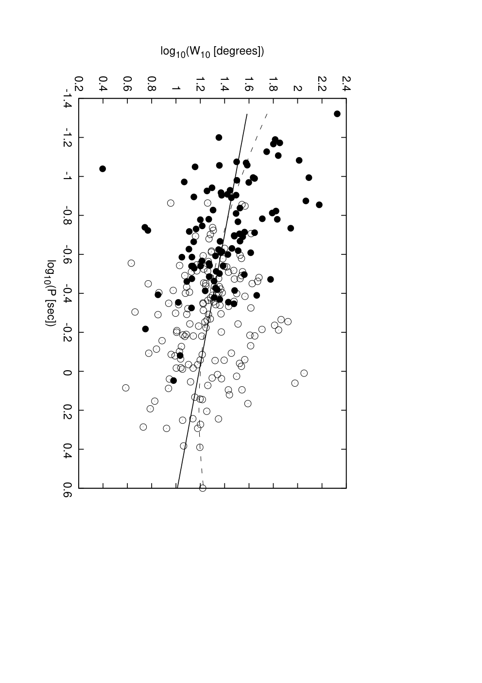
The measured pulse widths at 10% of the peak intensity () indeed show a slight anti-correlation with (Fig. 6), while there is no indication for a dependence with (not shown). The slope is measured by reduced fitting (the data points are weighted equally), which results in a slope of 44 4 The correlation is slightly different, although within the error identical to the value quoted in Weltevrede & Johnston (2008). This is because since the publication of that paper more timing observations have been added., comparable with the fit obtained from the data of Gould & Lyne (1998) by Weltevrede & Johnston (2008). The slope of the correlation is therefore slightly less than what is expected from theory. This conclusion, in combination with the period distribution of pulsars with interpulses, provides convincing evidence in favour for the evolution of the pulsar beam towards alignment with the rotation axis (Weltevrede & Johnston 2008).
If there is any deviation from a power law relationship between and , then it would be that the slope of the correlation is steeper for faster rotating pulsars. Although the fit of a second order polynomial through the data-points indeed show this trend, it is statistically not much better than the first order fit. High pulsars are in general spinning faster then low pulsars, and therefore one could conclude that the pulse widths of high pulsars have a stronger dependence on than the low pulsars. To illustrate this the pulsars with high and low values of are marked differently in Fig. 6. One could argue that there is not much evidence for a correlation for the low pulsars, while this is clearer for the high pulsars. But, as the fit second order polynomial was statistically not much better than the fit of a power law, this conclusion is also not significant. If this correlation exist, then it would suggest that the profile widths of the high pulsars follow the theoretical prediction more closely than those of the low pulsars, which could indicate that the emission geometry for high pulsars is more simple.
4.3 Pulse widths versus

In the previous subsection we found that is correlated with . One can expect that the correlation with is weaker, because was found to be uncorrelated with . Indeed, Fig. 7 shows that for most pulsars is as good as uncorrelated with . But remarkably, unlike in Fig. 6 there are a number of outliers which are clustered in relatively well defined regions in -space. These outliers are indicated by the ellipses and each group will be discussed separately below.
The first group of outliers are the pulsars in the ellipse at the left hand side of Fig. 7. Although the profiles are clearly wider than most pulse profiles, they form a continuous distribution with the narrower profiles. These low pulsars are PSRs J1034–3224, J1655–3048 and J2006–0807 (which have complex looking profiles) and PSRs J1133–6250 and J1137–6700 (which are doubles with a clear saddle between the components). The profiles of these pulsars are most likely broad because their beam is close to alignment with the rotation axis, making the beam intersect the line of sight for a relatively long fraction of the rotation period. There is evidence that the beam evolves to alignment with the rotation axis over time (e.g. Weltevrede & Johnston 2008), so it is not surprising that these aligned pulsars are old pulsars with low values. For two of these pulsars estimates for the angle between the magnetic axis and the rotation axis can be found in the literature. These polarization studies indeed suggest that the beam of PSRs J1034–3224 (Manchester et al., 1998) and J2006–0807 (Rankin, 1993b; Lyne & Manchester, 1988) are close to alignment.
The second group of pulsars with wide profiles are the pulsars with interpulses, which are marked with triangles in Fig. 7. These are PSRs J0834–4159, J0905–5127, B0906–49, B1124–60, J1549–4848, B1607–52, B1634–45, B1702–19, B1719–37, B1736–29, J1828–1101 and J1843–0702. The profiles of these pulsars are characterised by having an interpulse which is separated by approximately in pulse longitude from the main pulse. This separation is much larger than the widths of the main- and interpulse. The most natural explanation for these interpulses is that the emission of the main- and interpulse originates from opposite magnetic poles. These pulsars are concentrated to high values for . This is partially a selection effect in the sample of pulsars which are included in the Fermi timing program, but it has also shown by Weltevrede & Johnston (2008) that interpulses are more likely to be detected in young (high ) pulsars.
The third group of pulsars with wide profiles can also be found at the high end of Fig. 7. These are PSRs J1015–5719, B1259–63, J1803–2137, J1809–1917 and J1826–1334. Like the group of pulsars with wide profiles at the low end of the figure, this group appears to form a continuum with the pulsars with narrow profiles. We will refer to this group as the energetic wide beam pulsars. Their profiles show a double structure and they are exceptionally wide, but they are not separated by exactly in pulse longitude. In contrast to the group of interpulses, this separation is not much larger than the width of the individual components. The two components are often highly asymmetric with steep edges at opposite sides, making the profile as a whole to have a high degree of mirror symmetry. For some of these pulsars a weak bump is detected in between the components, which disappears at higher frequencies. The dependence of the PA on pulse longitude is usually simple and straight.
It is not clear if PSR B1055–52 should be classified as an energetic wide beam pulsar or a pulsar with an interpulse. On the one hand the separation between the main- and interpulse is larger than the width of the individual components, but on the other hand the components are very wide and the interpulse is not exactly away from the main pulse. The location of PSR B1055–52 in Fig. 7 (the lowest triangle at erg s-1) suggest that it is well separated from the other energetic wide beam pulsars, although the group of interpulse pulsars appear to have an overlap with the group of energetic wide beam pulsars. Especially the location of PSRs B0906–49 ( erg s-1) and J1828–1101 ( erg s-1) in the figure are consistent with both groups. Both these pulsars have interpulses at away from the main pulse and this separation is much larger than the component widths (the broad components of J1828–1101 at 20 cm are because of scatter broadening), which is good evidence that both interpulses are emitted from the opposite pole. For PSR B0906–49 the PA-swing is shown to be inconsistent with a wide cone interpretation (Kramer & Johnston 2008).
The energetic wide beam pulsars are among the pulsars with the highest values ( erg s-1), although it is not true that all pulsars with high values are also energetic wide beam pulsars. This is first of all shown by the overlap between the group of pulsars with interpulses and the energetic wide beam pulsars group. Secondly, PSR J1513–5908 which has the highest value in our sample, does not show any evidence of a double structure. Finally, PSR J1028–5819 is an extremely narrow double (Keith et al. 2008, point in the bottom left corner of Fig. 6). A high therefore appears to be an important parameter which allows an energetic pulsar to form a wide beam, but there must be more factors involved.
4.4 The intensity ratio of the components of high pulsars with double profiles
Johnston & Weisberg (2006) noted that the trailing component of well separated double profiles of high pulsars tend to dominate in total power (and in circular polarization as we will discuss below). This curious effect seems to be strongest for pulsars with erg s-1 (see for example PSR J1420–6048, Fig. ). The only exceptions are the Vela pulsar (which has no well separated double profile), PSR J1302–6350 (an energetic wide beam pulsars for which it is not clear which component is the trailing component) and PSR J1831–0952. Nevertheless, in the majority of the cases this correlation holds.
5 Polarization
5.1 Linear polarization


It has been pointed out by several authors that degree of linear polarization is high for high pulsars (e.g. Qiao et al. 1995; von Hoensbroech et al. 1998; Crawford et al. 2001; Johnston & Weisberg 2006). This correlation is clearly confirmed, as can be seen in Fig. 8. There is a transition from a low to a high degree of linear polarization which happens around erg s-1. Virtually all pulsars with erg s-1 have less than 50% linear polarization and for almost all pulsars with with erg s-1 this percentage is above 50%. There appears to be a transition region in between where pulsars can both have low and high degrees of polarization, although the transition is remarkably sharp and there are well defined spaces in the figure which are almost empty. The non-linearity of the degree of linear polarization versus is confirmed by fitting an arctan function through the data (solid curve in Fig. 8). This is done by minimizing the using the Levenberg-Marquardt algorithm (Marquardt, 1963) as implemented in Press et al. (1992) (the data points are weighted equally). The total is reduced by 20% compared with a linear fit, which shows that the step in the degree of linear polarization is important to consider. Adding higher order polynomial terms does not reduce the further, suggesting that the step is the most dominant deviation from non-linearity. The position of the steepest point in the fitted function occurs at .
The emission of pulsars is thought to be a combination of two orthogonally polarized modes (OPM, e.g. Manchester et al. 1975). This aspect of the emission can manifest itself in sharp jumps in the position angle (PA) over a small pulse longitude range. These jumps are thought to be sudden transitions from the domination of one mode to the other. Jumps in the PA-swing therefore indicates that both modes are present in the emission. The mixing of both modes at a certain longitude will lead to depolarization, so the presence of jumps in the PA-swing could be anti-correlated with the degree of polarization. By comparing the top and bottom panel of Fig. 9 one can see that the value at which the transition from a low to a high degree of polarization takes place coincides with the value after which pulsars do not have jumps in their PA. This is therefore important evidence that the increase in the degree of linear polarization with is caused by one OPM dominating the emission. Most high pulsars do not show OPM jumps, but the reverse is not always true. Low pulsars can have a low degree of linear polarization without evidence for OPM jumps.
There are three curious exceptions in Fig. 8 which do not follow the general trend. First of all PSRs J1509–5850 and J1833–0827 have a low degree of linear polarization while they have a high ( and erg s-1 respectively). However it must be noted that the leading and trailing components of PSR J1833–0827 are highly polarized at 10 cm. The degree of linear polarization of this pulsar shows a drop to zero in the middle of central component, which could indicate that there is a transition in the dominating OPM. The other exception is PSR J0108–1431, which has a low but is nevertheless highly polarized. This could suggest that this pulsar has some similarities with high energy pulsars.
All pulsars without a significant amount of measured degree of linear polarization fall below the erg s-1 line. The only exception is PSR J1055–6032, which appears to have a very low degree of polarization. The rule that high pulsars are highly polarized therefore is confirmed in the majority of all pulsars.
5.2 Emission heights
5.2.1 The emission height derived from the pulse width
The wider pulse profiles of high pulsars are often attributed to a larger emission height for those pulsars (e.g. Manchester 1996; Karastergiou & Johnston 2007). The divergence of the magnetic (dipole) field lines away from the magnetic axis makes the half opening angle of the beam scale with the square root of the emission height. Under the assumption that the beam of the pulsar is confined by the last open field lines it follows that
| (5) |
(e.g Lorimer & Kramer 2005), were is the emission height and the speed of light.
| Name | |||||
| [erg s-1] | [km] | [km] | [deg] | [km] | |
| J1015–5719 | – | 5160 | – | 6674 | |
| J1302–6350 | – | 3476 | – | 2279 | |
| J1803–2137 | 461 | 2967 | 8.3 | 6375 | |
| J1809–1917 | 130 | 1425 | 3.8 | 3948 | |
| J1826–1334 | 191 | 2522 | 4.5 | 4841 | |
| J0304+1932 | 75 | 562 | 0.1 | 66206 | |
| J0536–7543 | -21 | 1472 | -0.0 | 59444 | |
| J0614+2229 | 1051 | 99 | 7.5 | 15982 | |
| J0630–2834 | 118 | 2459 | 0.2 | 59376 | |
| J0631+1036 | 1087 | 278 | 9.1 | 13731 | |
| J0729–1448 | 1143 | 291 | 10.9 | 12008 | |
| J0742–2822 | 338 | 68 | 4.9 | 7957 | |
| J0835–4510 | 32 | 30 | 0.9 | 4263 | |
| J0908–4913 | 320 | 24 | 7.2 | 5094 | |
| J1048–5832 | -24 | 141 | -0.5 | 5901 | |
| J1105–6107 | 243 | 52 | 9.2 | 3015 | |
| J1119–6127 | 2082 | 1406 | 12.3 | 19455 | |
| J1123–4844 | 540 | 152 | 5.3 | 11682 | |
| J1253–5820 | 690 | 116 | 6.5 | 12191 | |
| J1320–5359 | 673 | 158 | 5.8 | 13347 | |
| J1359–6038 | 544 | 41 | 10.2 | 6084 | |
| J1420–6048 | 106 | 442 | 3.7 | 3253 | |
| J1531–5610 | 81 | 136 | 2.3 | 4018 | |
| J1535–4114 | 474 | 235 | 2.6 | 20654 | |
| J1637–4553 | 392 | 62 | 7.9 | 5667 | |
| J1701–3726 | 184 | 984 | 0.2 | 117118 | |
| J1705–3950 | -120 | 690 | -0.9 | 15218 | |
| J1709–4429 | 563 | 326 | 13.2 | 4889 | |
| J1733–3716 | 932 | 1969 | 6.6 | 16107 | |
| J1740–3015 | 818 | 31 | 3.2 | 28952 | |
| J1835–1106 | 445 | 93 | 6.4 | 7916 | |
| J1841–0345 | 353 | 415 | 4.2 | 9737 |
Wider beams are more likely to produce wide profiles, although the observed pulse width also depend on the orientation of the magnetic axis and the line of sight with respect to the rotation axis. The relevant parameters are the angle between the magnetic axis and the rotation axis and the angle between the line of sight and the rotation axis. A related angle is the impact parameter , which is the angle between the line of sight and the magnetic axis at its closest approach. For most pulsars it is extremely difficult to obtain reliable values for these angles, which makes it hard to derive the emission height from .
For a sample of pulsars with a random orientation of the magnetic axis and the line of sight both the and distribution are sinusoidal. Simulations using the model described in Weltevrede & Johnston (2008), show that the pulse width distribution for such a sample pulsars peaks at . Some pulsars will have wider profiles because the pulsar beam is more aligned with the rotation axis, while others will have narrower profiles because the line of sight grazes the beam. This implies that the typical pulse width of a large sample of pulsars which have random orientations of their spin and magnetic axis and have similar opening angles should be equal to . In other words, a typical profile width is equal to that which is expected for an orthogonal rotator () and a line of sight which makes a central cut through the emission beam (). For such geometry Eq. 5 can be rewritten to
| (6) |
which is the emission height for a typical random geometry assuming a magnetic dipole field and an active area of the polar cap which is set by the last open field lines.
5.2.2 The emission height derived from the PA-swing
An independent way to estimate the emission height is by measuring the shift of the PA-swing caused by the co-rotation of the emission region with the neutron star. In this method it is assumed that the PA-swing is described by the rotating vector model (RVM; Radhakrishnan & Cooke 1969). The position angle is then predicted to depend on the pulse longitude as
| (7) |
where and are the PA and the pulse longitude corresponding to the intersection of the line of sight with the fiducial plane (the plane containing the rotation and magnetic axis). The PA-swing is a S-shaped curve and its inflection point occurs at . The RVM fit is shown in the figures of Appendix A and B for the pulsars which have a roughly S-shaped PA-swing.
If the emission profile is symmetric around the magnetic axis, then one could expect the inflection point to coincide with the middle of the pulse profile. However, co-rotation causes the inflection point to be delayed with respect to the pulse profile. The pulse longitude difference between the middle of the profile and the inflection point of the PA-swing can be used to derive the emission height (Blaskiewicz et al. 1991)
| (8) |
The relative shift of the PA-swing with respect to the profile is independent of and (Dyks et al., 2004). If the emission height is too large it could be difficult to measure because the inflection point of the PA-swing is shifted beyond the edge of the pulse profile.
5.2.3 The derived emission heights

The emission height derived using the PA-swing () and using the pulse width () are both listed in Table 3. This only includes the pulsars which have a clear S-shaped PA-swing at 20 cm. The typical emission height is a few hundred km, which is similar to the emission height found by other authors (e.g. Blaskiewicz et al. 1991; Mitra & Rankin 2002). One can see that for some pulsars is negative, which is obviously impossible. This can be considered to be a clear warning that the emission heights for an individual source could be completely wrong, but one can nevertheless hope that they are meaningful in a statistical sense. In order to test this we calculated the Spearman rank-order correlation coefficient between and , which shows that there is no evidence for any correlation between these parameters. This is also evident from Fig. 10, where these quantities are plotted against each other. We are therefore forced to accept that even in a statistical sense the calculated emission heights are inconsistent, supporting the same conclusion reached by Mitra & Li (2004) based on six pulsars.
There are a number of reasons why the heights derived using the two methods could be inconsistent. If the beams are significant patchy, then the centroid of the profile is not related to the position of magnetic axis and both methods to derive emission heights will fail. We therefore made a distinction in Fig. 10 between the profiles which are clear doubles and other profiles, because the double structure could indicate that the pulsar beam is roughly symmetric around the magnetic axis. As one can see there is no noticeable difference in the distributions. Another effect that could be important is the effect of sweepback of the magnetic field lines. Dyks & Harding (2004) derived that the effect of sweepback can dominate over other effects of co-rotation at low altitudes, making it possible for the inflection point of the PA-curve to precede the profile centre. The PA-curve can also precede the profile in case of inward directed emission (Dyks et al. 2005).
Despite the inconsistency between the derived emission heights using both methods, it is not true that the emission heights are entirely random. Most pulsars show a positive emission height , indicating that the steepest slope of the PA-swing trails the centroid of the profile in most cases. In fact, Fig. 10 appears to show evidence that it is unlikely that both and are large. In Table 3 one can see that the emission of the energetic wide beam pulsars should come from near the light cylinder in order to explain the width of the pulse profiles (). However, the derived emission heights from the the PA-swing fits are not unusually large. In this list one could add the emission height of PSR J1015–5719, which is estimated by Johnston & Weisberg (2006) to be 380 km.
All the energetic wide beam pulsars with a derived emission height from the PA-swing can be found below the solid line in Fig. 10, as well as PSRs J1705–3950 and J1733–3716 which have similar profile shapes. It seems unlikely that they all have beams which are close to alignment with the rotation axis, which suggest a different reason for the large widths of the profiles of the energetic wide beam pulsars. Apparently the emission heights which are derived from the PA-swings of the energetic wide beam pulsars are systematically underestimated, or the heights derived from the profile widths are over estimated. The first case could be explained by magnetic field line sweepback when the emission height is low (Dyks & Harding 2004). The second case implies that the beams of these pulsars are wider than could be expected from the divergence of the dipole field lines. The widening of the pulsar beam could, at least in principle, be caused by propagation effects in the magnetosphere.
Another explanation for the deviation of the energetic wide beam pulsars from the line in Fig. 10 could be that the two methods estimate the emission heights at different locations in the magnetosphere. The method based on the profile width estimates the emission height at the edge of the of the beam, while the method using the PA-swing estimates the emission height of the more central regions of the beam. For the energetic wide beam pulsars was found to be systematically larger than , which can be interpreted as evidence for an increase in the emission height at the edge of the beam. This interpretation will be discussed in more detail in the following section.
Fig. 10 shows that besides the group of pulsars which have relatively large compared to , there is also a group in where the opposite is seen. An explanation could be that for those pulsars only a fraction of the polar cap is active (e.g. Kijak & Gil 1997). Support for this interpretation is that the profiles of a number of pulsars in this group are argued to be produced by partial cones, including PSR J0543+2329 (Weisberg et al. 2004), J0614+2229 (Johnston et al. 2007) and J0659+1414 (Everett & Weisberg 2001).
5.3 Circular polarization

Unlike the degree of linear polarization the degree of circular polarization appears to be unaffected by . Also the fraction of pulsar which are left- and right-hand circularly polarized is about 50 per-cent for both the high and low pulsars.
Johnston & Weisberg (2006) noted that, besides the total intensity, also the degree of circular polarization usually dominates in the trailing components of high pulsars with well separated double profiles. This correlation is also clearly confirmed in our data for all pulsars with an erg s-1. The only clear counter example in our data-set could be PSR J1705–1906 ( erg s-1), which has a high degree of circular polarization in the leading half of the profile. However, it must be noted that the single pulse modulation properties of this pulsar suggest that the leading component is not the leading component of a double, but rather a precursor to a blended double which forms the trailing half of the profile (Weltevrede et al. 2007).
Remarkable correlations have been reported between the sign of the circular polarization and the sign of the slope of the PA-swing. According to Radhakrishnan & Rankin (1990) the sign of the slope of the PA-swing is correlated with the sign of the circular polarization for pulsars which are cone dominated and for which the sign of the circular polarization is the opposite in the two components. But Han et al. (1998) did not confirm this correlation. Instead they propose that there is a correlation between the sign of the circular polarization and the sign of the slope of the PA-swing for cone dominated pulsars which have the same sign of circular polarization. Our data does not show much evidence for either correlation. Compare for instance the plots for PSR J1826–1334 (positive circular polarization, decreasing PA-swing) with PSR J1733–3716 (negative circular polarization, decreasing PA-swing).
6 Discussion
6.1 Extended radio emission regions?
We concluded that the differences in the pulse profile morphology of the high and low pulsars is in general rather subtle, without an objectively measurable discriminator between them. An exception is what we call the group of energetic wide beam pulsars, which do have distinct profile properties and which will be discussed separately below. The measured slope of the correlation appears to be flatter than the theoretical slope. It is far from straight-forward to link the deviation of the slope to a physical mechanism. For example, as explained in Weltevrede & Johnston (2008), the measured slope depends on the details of the evolution of the pulsar spin-down and the alignment of the magnetic axis with the rotation axis. If the active area of the polar cap is influenced by other factors than just the opening angle of the last open field lines, or if the emission height varies from pulsar to pulsar, one can expect to observe its effects in the correlation. There is some marginal evidence that the slope of the correlation is steeper for high pulsars, suggesting that for high pulsars these other factors are less important.
If one believes that the emission geometry is simpler for high pulsars, one can ask the question of what is causing this. One factor that could affect the complexity of profiles is the emission height. Complexity could arise because of multiple distinct emission heights within the beam (Karastergiou & Johnston 2007). In their model high pulsars have only one emission height which is similar for different pulsars. However, one could also make the argument for an opposite effect. Maybe the emission of high pulsars is not emitted from a well defined height, but rather from an extended height range. This would mean that the observed profiles of high pulsars are a superposition of profiles emitted from a continuum of heights. The observed sum of those profiles (shifted with respect to each other by aberration and retardation) will have less complexity because they are blurred out. Not only are the profiles expected to be less complex in this scenario, but there is also not much room to vary the emission height from pulsar to pulsar if the height range is large. This would make the correlation follow the prediction more closely. Large emission height ranges are typical for high energy models, such as the slot gap models (e.g. Muslimov & Harding 2004a) or the two pole caustic models (Dyks & Rudak 2003), hence there could be parallels with the radio emission for high pulsars. These parallels could be even more relevant for the energetic wide beam pulsars.
6.2 The energetic wide beam pulsars
As discussed by e.g. Manchester (1996), there is a group of young pulsars which can be found among the highest pulsars which have very wide profiles with often steep edges. The profiles are clearly mirror symmetric, suggesting that the components are the two sides of a single beam rather than two beams from opposing magnetic poles. This interpretation is also suggested by the frequency evolution of PSR B1259–63 (Manchester & Johnston 1995). Because these objects are young, the typical orientation of the magnetic axis is not expected to be very different for the highest pulsars and those with intermediate values, which suggests that some pulsars with high values can have very different beams compared with other pulsars.
An interesting analogue can be drawn between the radio profiles of energetic wide beam pulsars and the high energy profiles of pulsars. High energy profiles can also be wide doubles which often have sharp edges (e.g. Thompson 2004). The pulsars which produce high energy emission are the pulsars with high values, so there could be a direct link between the high energy pulsars and the energetic wide beam pulsars. Maybe the radio emission and the high energy emission are produced at the same location in the magnetosphere. The sharp edges of the high energy profiles are often explained by caustics which form because of the combined effect of field line curvature, aberration and retardation (e.g. Morini 1983). These caustics occur when the emission is produced high in the magnetosphere over a large altitude range and if the magnetic axis is not aligned to the rotation axis (e.g. Dyks & Rudak 2003). If the radio emission and -ray emission would come from similar locations, one would expect the radio and -ray profiles to look alike. Hopefully the Fermi satellite will find high energy counterparts for these pulsars which allows a test of this hypothesis.
Another way to produce profiles with sharp edges could be the combination of refraction of radio waves in pulsar magnetospheres in combination with an emission height which is different for different field lines (Weltevrede et al. 2003). Only the ordinary wave mode is refracted (e.g. Barnard & Arons 1986) or scattered (Petrova 2008) in the magnetosphere. The profiles of the energetic wide beam pulsars can therefore be expected to be dominated by one polarization mode, which could potentially also explain their high degree of linear polarization. The unpolarized bump which is observed in the middle of some of these profiles could be the un-refracted part of the beam, which is depolarized because the presence of the extra-ordinary mode. These central components are strongest at lower frequencies, consistent with the steeper spectral index which is often observed for the central components of pulse profiles (e.g. Rankin 1983). However, it remains to be seen if propagation effects can be strong enough to explain the extreme pulse widths which are observed.
The emission geometry appears to be different for high pulsars and is possibly more similar to that of the high energy emission. However, not all pulsars with high values produce these extremely wide profiles. Apparently only a subset of the high pulsars have emission geometries which are very different from normal radio pulsars. A high is therefore an important parameter required for the energetic wide beam pulsars, but not the only one. For instance, maybe only certain configurations of the plasma distributions enlarge the beam via propagation effects or maybe not all pulsars have a slot gap which produces radio emission. It must also be noted that, like the high radio pulsars, not all the high energy pulse profiles of pulsars are doubles (e.g. PSR B1706–44).
6.3 Emission heights
There is no evidence that pulsars with large emission heights (derived from their PA-swing) have wider profiles. It is therefore not clear what the physical meaning of these emission heights is. There are many reasons why the derived emission heights could be wrong, including asymmetric beams, partially active polar caps or sweepback of the magnetic field lines. Also if the PA-swing of emission which is emitted far out in the magnetosphere the PA can be expected to deviate from the rotating vector model. For instance, the PA-swing for the outer gap model is predicted to have the steepest slope near the edges of the profile (Romani & Yadigaroglu 1995), rather then at the pulse longitude corresponding to the location of the magnetic axis. This would complicate the calculation of emission heights from the observed PA-swing considerably. Nevertheless, the fact that most PA-swings trail the centroid of the profile suggest that the derived emission heights do carry some information.
The emission of the energetic wide beam pulsars should come from near the light cylinder in order to explain the width of the pulse profiles. However, the derived emission heights from the PA-swing fits seem to suggest that the emission heights are not unusually large. This can be seen as support that the beams of energetic wide beam pulsars are wide because of propagation effects instead of caused by a large emission height. An alternative interpretation is that the emission height at the edge of the beam is much larger than in the centre of the beam. This would fit in nicely with the result of Gupta & Gangadhara (2003), who concluded that the outer components of PSR B0329+54 are emitted from higher in the magnetosphere. It also fits in nicely with the hypothesis that the emission of the energetic wide beam pulsars comes from an extended emission height range, making the emission geometry very similar to the slot gap model.
6.4 Interpulse problem?
The conclusion that the beams of energetic wide beam pulsars are large appears to be unavoidable. If this is the case, than one would expect that it is very likely for the line of sight to intersect the beams of both poles of the pulsar. Using the model described by Weltevrede & Johnston (2008) the probability for the line of sight to intersect both beams is predicted to be 64%, assuming and a random orientation of the magnetic axis and the line of sight. However, there is no clear example of an energetic wide beam pulsar which has a (double peaked) interpulse. The “interpulse problem” is then why we do not observe the interpulses of the energetic wide beam pulsars.
It is argued by Manchester (1996) that the steep edges form the outer edge of an extremely wide beam, which would make the peak-to-peak separation of the profiles wider than . In that case the weak bumps observed for some of these pulsars are then separated by half a rotational phase from the centre of the profile, which would make them interpulses. However, because the bumps fill in the region in between the sharp edges, it seems more likely that the sharp edges form the inner edges of a wide beam. In that case the profiles are less wide and the bump forms the centre of the same wide beam.
The interpulse problem suggests that the beam sizes are different for the magnetic poles of the energetic wide beam pulsars. As discussed above, not all profiles of high pulsars have wide components. This implies that other criteria have to be met in order to make the beams wide. These criteria are not necessarily met simultaneously for both poles, which would reduce the fraction of pulsars with interpulses. The very different shape of the main- and interpulse of PSR B1055–52 show that interpulse beams can have very different shapes, hence possibly also very different sizes. Only 5 of the 26 pulsars with an erg s-1 in Fig. 7 are classified to be energetic wide beam pulsars. Therefore the chance that both poles produces a wide beam is expected to be only if the chance of producing a wide beam is independent for each pole.
A more extreme point of view to solve the interpulse problem is put forward by Manchester (1996) who argues, following Manchester & Lyne (1977), that all pulsars only have one active wide beam. Although this would trivially solve the interpulse problem, it does not explain the concentration of main- interpulse separations near (see Fig. 7).
6.5 Polarization
The degree of linear polarization is found in several studies to increase with . Such behaviour is predicted for the natural wave modes in the cold plasma approximation (von Hoensbroech et al. 1998). One of the most surprising results of this paper is the sudden increase in the degree of linear polarization with . This suggest that pulsars can be separated into two groups which have distinct physical properties. This could either be in the structure of the magnetosphere or the physics of the emission mechanism itself. It is remarkable that over 7 orders of magnitude in the degree in linear polarization is the only thing that is clearly changing.
It has been shown that the degree of polarization is clearly related to the presence of OPM transitions in the PA-swing. The two plasma modes (X-mode and O-mode) can be expected to be separated more in pulse longitude for high pulsars, because the difference in their refractive indices is larger (e.g. von Hoensbroech et al. 1998). This could prevent the modes from mixing, and therefore prevent depolarization. However, the fact that high pulsars are less likely to show jumps in their PA-swing suggests that they only effectively generate one of the modes. Johnston et al. (2005) found that the velocity vectors of most pulsars make an angle close to either or with the PA of the linear polarization (measured at the inflection point). This is interpreted as evidence for alignment of the rotation axis of the star with its proper motion vector and the bimodal nature of the distribution of angles is interpreted to be due to the domination of different plasma modes for different stars. This result therefore suggest that if the emission of high pulsars is dominated by one mode, it could be either of the two for different pulsars. If the profiles of the energetic wide beam pulsars are widened by refraction, than their emission should be dominated by the O-mode which can be refracted in the pulsar magnetosphere.
A very different interpretation of the sudden increase of the degree of linear polarization with is based on the fact that the at the transition is very similar to the death line for curvature radiation (Harding & Muslimov 2002). This death line could potentially cause a sudden change in for instance the plasma distribution in the magnetosphere (which is responsible for the refraction of the plasma waves), or it could possibly change the emission mechanism which is responsible for the radio emission. The possible link between the degree of linear polarization of the radio emission and the mechanism for the production of the high energy emission could therefore suggest that the -ray efficiency is correlated with the degree of linear polarization in the radio band. It would therefore be extremely interesting to find out if a pulsar like PSR J0108–1431, which is highly polarized with a low , can be detected by the Fermi satellite.
6.6 Circular polarization
The trend noted by Johnston & Weisberg (2006) that the degree of circular polarization is usually higher in the second component of doubles is clearly present in our data as well. It is a possibility that this is a result of the co-rotation velocity of the emission region. As shown by for instance Dyks (2008), particles travelling along the magnetic field lines of a rotating dipole will follow stronger curved paths (in the inertial observer frame) at the leading half of the pulse profiles compared to the trailing half of the pulse profile. This is the reason why the observed PA-swing appears to be shifted with respect to the pulse profile (equation 8). The degree of circular polarization is in general highest in the central parts of the pulse profile, there where the curvature of the field lines is weakest. This could therefore suggest that the location of the highest degree of circular polarization is, like the PA-swing, shifted to later times by co-rotation.
7 Conclusions
In this paper we present and discuss the polarization profiles of a large sample of young, highly energetic pulsars which are regularly observed with the Parkes telescope. This sample is compared with a sample of a similar number of low objects in order to draw general conclusions about their differences.
There is some evidence that the total intensity profiles of high pulsars are slightly simpler based on a classification by eye. However, there is no difference in the complexity of the mathematical decomposition of the profiles, the amount of overlap between the components of doubles or the degree of profile symmetry. We therefore conclude that differences in the total intensity pulse morphology between high and low pulsars are in general rather subtle. High pulsars appear to show a stronger correlation which is closer to the theoretical expectation, suggesting that for high pulsars there are less complicating factors in the emission geometry.
A much more pronounced difference between high and low pulsars is the degree of polarization. The degree of polarization was already known to increase with , but our data shows there is a rapid transition between relatively unpolarized low pulsars and highly polarized high pulsars. The increase in the degree of polarization is related to the absence of OPM jumps. Refraction of the radio emission is expected to be more effective in the magnetosphere of high pulsars, which could prevent depolarization because of mixing of the plasma modes. The absence of OPM jumps suggest that one of the two modes (not necessarily the same for different pulsars) dominates over the other. The of the transition is very similar to the death line for curvature radiation, which could be the reason why the transition is relatively sharp. This potential link between the high energy radiation and the radio emission could mean that the -ray efficiency is correlated with the degree of linear polarization in the radio band.
The degree of circular polarization is in general higher in the second component of doubles. This remarkable correlation is possibly caused by the effect of co-rotation on the curvature of the field lines in the inertial observer frame, making this effect very similar to the shift of the PA-swing predicted for a finite emission height. In addition, the trailing component usually dominates in total power.
The distribution clearly shows sub-groups which are not visible in the pulse distribution, suggesting that is an important physical parameter for pulsar magnetospheres. Besides a group of pulsars which probably have beams aligned with the rotation axis and a group of pulsars with interpulses which are probably orthogonal rotators there is a group of energetic wide beam pulsars. These young pulsars have very wide profiles with often steep edges which are likely to be emitted from a single pole.
The profile properties of the energetic wide beam pulsars are similar to those of the high energy profiles, suggesting another possible link with the high energy emission. We therefore propose that the emission of these pulsars could come, like the high energies, from extended parts of the magnetosphere. The extended height range from where the emission is emitted will smear out the complex features of the profiles. A large height range could also prevent the emission height to vary much from pulsar to pulsar, which would result in a stronger correlation for high pulsars, as is indeed observed. If the radio emission and -ray emission of these pulsars indeed come from similar locations in the magnetosphere, one would expect the radio and -ray profiles to look alike, something that potentially can be tested by the Fermi satellite.
An alternative mechanism to produce the profiles of the energetic wide beam pulsars could be the combination of refraction (or scattering) of radio waves in pulsar magnetospheres with an emission height which is different for different field lines (Weltevrede et al. 2003). Refraction (and scattering) is most severe for the ordinary wave mode, suggesting that these profiles are dominated by one polarization mode. This would be consistent with the high degree of linear polarization observed for these pulsars. The unpolarized bump in the middle of the profiles of the energetic wide beam pulsars could be the un-refracted part of the beam, which is depolarized because the mixing of the plasma modes.
Measurements of the emission height could potentially discriminate between the refraction model and the extended emission height model for the energetic wide beam pulsars. There is no evidence that pulsars with large emission heights (derived from their PA-swing) have wider profiles. It is therefore not clear what the physical meaning of these emission heights are. It could supports the idea that the beams of energetic wide beam pulsars are wide because of refraction instead of caused by a large emission heights. However, it could also mean that the emission height of the outer parts of the beam is much larger than for the central parts, making the emission geometry similar to that of a slot gap.
Acknowledgments
The authors would like to thank the referee, Axel Jessner, for his useful comments on this paper. The Australia Telescope is funded by the Commonwealth of Australia for operation as a National Facility managed by the CSIRO.
References
- Barnard & Arons (1986) Barnard J. J., Arons J., 1986, ApJ, 302, 138
- Biggs (1990) Biggs J. D., 1990, MNRAS, 245, 514
- Blaskiewicz et al. (1991) Blaskiewicz M., Cordes J. M., Wasserman I., 1991, ApJ, 370, 643
- Cheng et al. (1986) Cheng K. S., Ho C., Ruderman M., 1986, ApJ, 300, 500
- Crawford et al. (2001) Crawford F., Manchester R. N., Kaspi V. M., 2001, AJ, 122, 2001
- D’Amico et al. (1998) D’Amico N., Stappers B. W., Bailes M., Martin C. E., Bell J. F., Lyne A. G., Manchester R. N., 1998, MNRAS, 297, 28
- Daugherty & Harding (1996) Daugherty J. K., Harding A. K., 1996, ApJ, 458, 278
- Dyks (2008) Dyks J., 2008, astro-ph/0806.0554
- Dyks et al. (2005) Dyks J., Fra̧ckowiak M., Słowikowska A., Rudak B., Zhang B., 2005, ApJ, 633, 1101
- Dyks & Harding (2004) Dyks J., Harding A. K., 2004, ApJ, 614, 869
- Dyks & Rudak (2003) Dyks J., Rudak B., 2003, ApJ, 598, 1201
- Dyks et al. (2004) Dyks J., Rudak B., Harding A. K., 2004, ApJ, 607, 939
- Everett & Weisberg (2001) Everett J. E., Weisberg J. M., 2001, ApJ, 553, 341
- Gil et al. (1993) Gil J. A., Kijak J., Seiradakis J. H., 1993, A&A, 272, 268
- Gonthier et al. (2007) Gonthier P. L., Story S. A., Clow B. D., Harding A. K., 2007, Astrophys. Space Sci., 309, 245
- Gould & Lyne (1998) Gould D. M., Lyne A. G., 1998, MNRAS, 301, 235
- Gupta & Gangadhara (2003) Gupta Y., Gangadhara R. T., 2003, ApJ, 584, 418
- Han et al. (1998) Han J. L., Manchester R. N., Xu R. X., Qiao G. J., 1998, MNRAS, 300, 373
- Harding & Muslimov (2001) Harding A. K., Muslimov A. G., 2001, ApJ, 556, 987
- Harding & Muslimov (2002) Harding A. K., Muslimov A. G., 2002, ApJ, 568, 862
- Hotan et al. (2004) Hotan A. W., van Straten W., Manchester R. N., 2004, Publications of the Astronomical Society of Australia, 21, 302
- Huguenin et al. (1971) Huguenin G. R., Manchester R. N., Taylor J. H., 1971, ApJ, 169, 97
- Johnston et al. (2005) Johnston S., Hobbs G., Vigeland S., Kramer M., Weisberg J. M., Lyne A. G., 2005, MNRAS, 364, 1397
- Johnston et al. (2007) Johnston S., Kramer M., Karastergiou A., Hobbs G., Ord S., Wallman J., 2007, MNRAS, 381, 1625
- Johnston et al. (1992) Johnston S., Lyne A. G., Manchester R. N., Kniffen D. A., D’Amico N., Lim J., Ashworth M., 1992, MNRAS, 255, 401
- Johnston & Weisberg (2006) Johnston S., Weisberg J. M., 2006, MNRAS, 368, 1856
- Karastergiou & Johnston (2007) Karastergiou A., Johnston S., 2007, MNRAS, 380, 1678
- Karastergiou et al. (2005) Karastergiou A., Johnston S., Manchester R. N., 2005, MNRAS, 359, 481
- Keith et al. (2008) Keith M. J., Johnston S., Kramer M., Weltevrede P., Watters K. P., Stappers B. W., 2008, MNRAS, in press (astro-ph/0807.2088)
- Kijak & Gil (1997) Kijak J., Gil J., 1997, MNRAS, 288, 631
- Kramer & Johnston (2008) Kramer M., Johnston S., 2008, MNRAS, in press (astro-ph/0807.5013)
- Kramer et al. (1994) Kramer M., Wielebinski R., Jessner A., Gil J. A., Seiradakis J. H., 1994, A&AS, 107, 515
- Kramer et al. (1998) Kramer M., Xilouris K. M., Lorimer D. R., Doroshenko O., Jessner A., Wielebinski R., Wolszczan A., Camilo F., 1998, ApJ, 501, 270
- Lorimer & Kramer (2005) Lorimer D. R., Kramer M., 2005, Handbook of Pulsar Astronomy. Cambridge University Press
- Lyne & Manchester (1988) Lyne A. G., Manchester R. N., 1988, MNRAS, 234, 477
- Manchester (1996) Manchester B. N., 1996, in Johnston S., Walker M. A., Bailes M., eds, ASP Conf. Ser. 105: IAU Colloq. 160: Pulsars: Problems and Progress Wide Beams from Young Pulsars (or One Pole for All). pp 193–+
- Manchester et al. (1998) Manchester R. N., Han J. L., Qiao G. J., 1998, MNRAS, 295, 280
- Manchester et al. (2005) Manchester R. N., Hobbs G. B., Teoh A., Hobbs M., 2005, AJ, 129, 1993
- Manchester & Johnston (1995) Manchester R. N., Johnston S., 1995, ApJ, 441, L65
- Manchester & Lyne (1977) Manchester R. N., Lyne A. G., 1977, MNRAS, 181, 761
- Manchester et al. (1975) Manchester R. N., Taylor J. H., Huguenin G. R., 1975, ApJ, 196, 83
- Marquardt (1963) Marquardt D., 1963, Journal of the Society for Industrial and Applied Mathematics, 11, 431
- Mitra & Li (2004) Mitra D., Li X. H., 2004, A&A, 421, 215
- Mitra & Rankin (2002) Mitra D., Rankin J. M., 2002, ApJ, 577, 322
- Morini (1983) Morini M., 1983, MNRAS, 202, 495
- Muslimov & Harding (2004a) Muslimov A. G., Harding A. K., 2004a, ApJ, 606, 1143
- Muslimov & Harding (2004b) Muslimov A. G., Harding A. K., 2004b, ApJ, 617, 471
- Pellizzoni et al. (2008) Pellizzoni A., Pilia M., Possenti A., Fornari F., Caraveo P., Del Monte E., Mereghetti S., Tavani M., Argan A., Trois e. a., 2008, ApJ, submitted
- Petrova (2008) Petrova S. A., 2008, MNRAS, 384, L1
- Press et al. (1992) Press W. H., Teukolsky S. A., Vetterling W. T., Flannery B. P., 1992, Numerical Recipes: The Art of Scientific Computing, 2nd edition. Cambridge University Press, Cambridge
- Qiao et al. (1995) Qiao G. J., Manchester R. N., Lyne A. G., Gould D. M., 1995, MNRAS, 274, 572
- Radhakrishnan & Cooke (1969) Radhakrishnan V., Cooke D. J., 1969, Astrophys. Lett., 3, 225
- Radhakrishnan & Rankin (1990) Radhakrishnan V., Rankin J. M., 1990, ApJ, 352, 258
- Rankin (1983) Rankin J. M., 1983, ApJ, 274, 333
- Rankin (1993a) Rankin J. M., 1993a, ApJ, 405, 285
- Rankin (1993b) Rankin J. M., 1993b, ApJS, 85, 145
- Romani (1996) Romani R. W., 1996, ApJ, 470, 469
- Romani & Yadigaroglu (1995) Romani R. W., Yadigaroglu I.-A., 1995, ApJ, 438, 314
- Smith et al. (2008) Smith D., Guillemot L., Camilo F., Cognard I., Dumora D., Espinoza C., et al. 2008, A&A, submitted
- Thompson (2004) Thompson D. J., 2004, in Cheng K. S., Romero G. E., eds, Cosmic Gamma-Ray Sources Vol. 304 of Astrophysics and Space Science Library, Gamma ray pulsars. pp 149–+
- van Straten (2004) van Straten W., 2004, Astrophys. J. Supp. Series, 152, 129
- von Hoensbroech et al. (1998) von Hoensbroech A., Lesch H., Kunzl T., 1998, A&A, 336, 209
- von Mises (1918) von Mises R., 1918, Physikalische Zeitschrift, 19, 490
- Weisberg et al. (2004) Weisberg J. M., Cordes J. M., Kuan B., Devine K. E., Green J. T., Backer D. C., 2004, Astrophys. J. Supp. Series, 150, 317
- Weltevrede & Johnston (2008) Weltevrede P., Johnston S., 2008, MNRAS, 387, 1755
- Weltevrede et al. (2003) Weltevrede P., Stappers B. W., van den Horn L. J., Edwards R. T., 2003, A&A, 412, 473
- Weltevrede et al. (2007) Weltevrede P., Wright G. A. E., Stappers B. W., 2007, A&A
Appendix A Polarization figures at both 10 and 20 cm
The astro-ph version is missing 528 figures due to file size restrictions. Please download the paper including the appendices from http://www.atnf.csiro.au/people/pulsar/wj08b.pdf.
Appendix B Polarization figures only at 20 cm
The astro-ph version is missing 528 figures due to file size restrictions. Please download the paper including the appendices from http://www.atnf.csiro.au/people/pulsar/wj08b.pdf.
Appendix C Table with the profile properties
| Name | Class | Scat. | Sym. | Fig. | ||||||||
|---|---|---|---|---|---|---|---|---|---|---|---|---|
| [cm] | [sec] | [°] | [°] | [%] | [%] | |||||||
| J0034–0721 | 20 | 959 | S | 217 | N | 12.4 | 34.5 | 2 | 0.964 | 7.8 0.8 | 3.4 0.5 | |
| J0051+0423 | 20 | 3838 | D | 32 | N | 31.1 | 42.3 | 0.926 | ||||
| J0108–1431 | 10 | 6565 | S | 54 | N | 10.5 | 26.3 | 0.978 | 40.0 3.9 | |||
| J0108–1431 | 20 | 19731 | S | 186 | N | 12.2 | 28.5 | 2 | 0.990 | 71.1 1.1 | 13.7 0.8 | |
| J0134–2937 | 20 | 960 | D | 238 | N | 5.6 | 18.2 | 4 | 0.803 | 41.9 0.8 | -21.1 0.5 | |
| J0151–0635 | 20 | 959 | D | 51 | N | 29.3 | 39.0 | 0.884 | 22.0 2.5 | |||
| J0152–1637 | 20 | 958 | D | 506 | N | 6.8 | 9.8 | 3 | 0.939 | 12.1 0.3 | -2.0 0.2 | |
| J0206–4028 | 20 | 960 | D | 52 | N | 3.5 | 10.1 | 0.973 | 6.9 2.2 | |||
| J0211–8159 | 20 | 1918 | S | 18 | N | 20.6 | 37.6 | 0.887 | ||||
| J0255–5304 | 20 | 960 | D | 157 | N | 6.3 | 8.7 | 2 | 0.978 | 6.5 0.9 | -6.3 0.5 | |
| J0304+1932 | 20 | 959 | D | 298 | N | 11.3 | 15.8 | 2 | 0.945 | 31.5 0.5 | 13.0 0.4 | |
| J0401–7608 | 10 | 5455 | D | 122 | N | 12.9 | 17.9 | 2 | 0.964 | 20.6 1.3 | ||
| J0401–7608 | 20 | 7582 | M | 383 | N | 13.8 | 18.0 | 2 | 0.989 | 27.1 0.4 | ||
| J0448–2749 | 20 | 960 | S | 58 | N | 9.2 | 16.7 | 0.992 | 19.7 3.6 | -14.3 2.6 | ||
| J0450–1248 | 20 | 960 | D | 50 | N | 20.5 | 30.0 | 0.990 | 16.7 3.5 | |||
| J0459–0210 | 20 | 958 | D | 38 | N | 3.4 | 13.2 | 0.890 | -9.4 3.1 | |||
| J0520–2553 | 20 | 960 | D | 51 | N | 15.1 | 19.6 | 0.796 | 14.0 3.3 | |||
| J0525+1115 | 20 | 959 | M | 103 | N | 14.4 | 17.6 | 3 | 0.894 | 9.2 1.7 | 6.8 1.2 | |
| J0533+0402 | 20 | 1918 | S | 81 | N | 5.5 | 10.1 | 0.996 | 7.9 2.4 | |||
| J0536–7543 | 10 | 3567 | M | 118 | N | 16.6 | 25.3 | 3 | 0.918 | 29.3 1.4 | -23.2 1.0 | |
| J0536–7543 | 20 | 10775 | M | 1557 | N | 17.0 | 27.0 | 4 | 0.899 | 47.5 0.1 | -11.1 0.1 | |
| J0540–7125 | 20 | 1916 | M | 29 | N | 9.6 | 15.9 | 0.895 | ||||
| J0543+2329 | 20 | 809 | D | 194 | N | 7.8 | 23.3 | 2 | 0.971 | 43.2 1.0 | -8.9 0.7 | |
| J0601–0527 | 20 | 960 | D | 138 | N | 16.1 | 21.8 | 2 | 0.888 | 28.8 1.1 | 2.9 0.8 | |
| J0614+2229 | 10 | 180 | S | 47 | N | 8.0 | 14.6 | 0.983 | 46.3 3.8 | 16.8 2.8 | ||
| J0614+2229 | 20 | 807 | S | 197 | N | 7.4 | 13.5 | 1 | 0.997 | 69.8 0.9 | 18.5 0.6 | |
| J0624–0424 | 20 | 899 | M | 167 | N | 2.0 | 21.9 | 4 | 0.736 | 21.7 0.8 | 6.4 0.6 | |
| J0630–2834 | 10 | 2396 | S | 297 | N | 16.3 | 30.5 | 3 | 0.998 | 24.5 0.6 | -4.2 0.4 | |
| J0630–2834 | 20 | 5776 | S | 871 | N | 18.4 | 34.9 | 3 | 0.999 | 44.8 0.2 | -3.3 0.1 | |
| J0631+1036 | 20 | 1919 | M | 78 | N | 8.2 | 24.4 | 0.987 | 82.6 2.2 | |||
| J0636–4549 | 20 | 1917 | S | 20 | N | 3.2 | 5.9 | 0.973 | ||||
| J0656–2228 | 20 | 900 | S | 50 | N | 4.7 | 8.7 | 0.985 | ||||
| J0656–5449 | 20 | 960 | S | 30 | N | 10.9 | 20.0 | 0.939 | -17.9 5.3 | |||
| J0659+1414 | 10 | 179 | S | 87 | N | 14.8 | 32.1 | 0.986 | 49.7 2.3 | -14.5 1.7 | ||
| J0659+1414 | 20 | 717 | S | 111 | N | 13.9 | 30.3 | 1 | 0.984 | 70.5 1.7 | -15.0 1.2 | |
| J0709–5923 | 20 | 959 | S | 26 | N | 4.1 | 7.5 | 0.966 | ||||
| J0719–2545 | 20 | 959 | S | 62 | N | 6.2 | 11.3 | 0.917 | 10.0 2.9 | 13.6 2.1 | ||
| J0729–1448 | 10 | 1779 | D | 34 | N | 20.0 | 28.0 | 0.946 | 78.9 5.4 | |||
| J0729–1448 | 20 | 5146 | D | 94 | N | 10.7 | 26.7 | 0.886 | 72.1 1.9 | 16.6 1.2 | ||
| J0729–1836 | 20 | 960 | D | 88 | N | 9.8 | 18.5 | 0.896 | 19.6 2.1 | -6.1 1.5 | ||
| J0742–2822 | 10 | 430 | M | 448 | N | 9.9 | 16.0 | 3 | 0.961 | 80.6 0.4 | -4.2 0.3 | |
| J0742–2822 | 20 | 3296 | M | 2463 | N | 9.9 | 15.9 | 3 | 0.972 | 81.4 0.1 | -1.7 0.0 | |
| J0745–5353 | 10 | 2079 | S | 96 | N | 17.7 | 32.4 | 0.992 | 11.9 1.8 | |||
| J0745–5353 | 20 | 10012 | S | 476 | N | 18.2 | 33.6 | 2 | 0.997 | 20.8 0.4 | 3.6 0.3 | |
| J0749–4247 | 20 | 959 | S | 44 | N | 4.8 | 8.8 | 0.963 | 17.9 4.1 | |||
| J0820–3921 | 20 | 1920 | S | 26 | N | 24.2 | 44.4 | 0.941 | 23.2 6.2 | 15.5 4.2 | ||
| J0821–3824 | 20 | 1079 | S | 30 | N | 17.1 | 31.2 | 0.934 | ||||
| J0821–4221 | 20 | 960 | D | 43 | N | 13.8 | 22.5 | 0.933 | ||||
| J0834–4159 | 10 | 3580 | S | 15 | N | 10.8 | 20.3 | 0.875 | ||||
| J0834–4159 | 20 | 15737 | S | 59 | N | 13.3 | 23.4 | 0.965 | -11.7 2.3 | |||
| J0834–4159I | 20 | 15737 | S | 17 | N | 15.5 | 28.4 | 0.907 | ||||
| J0835–4510 | 10 | 820 | D | 9275 | N | 6.4 | 17.2 | 4 | 0.833 | 89.6 0.0 | -17.5 0.0 | |
| J0835–4510 | 20 | 6496 | D | 26906 | N | 6.0 | 14.3 | 3 | 0.949 | 90.0 0.0 | -6.0 0.0 | |
| J0838–2621 | 20 | 1919 | D | 31 | N | 10.0 | 35.2 | 0.886 | ||||
| J0843–5022 | 20 | 960 | S | 36 | N | 10.2 | 18.7 | 0.968 | ||||
| J0849–6322 | 20 | 1919 | D | 68 | N | 6.5 | 22.7 | 0.900 | 24.8 2.6 | -9.1 1.7 | ||
| J0855–4644 | 10 | 3560 | S | 12 | N | 38.0 | 70.1 | 0.796 | ||||
| J0855–4644 | 20 | 29519 | S | 49 | N | 35.5 | 65.4 | 0.953 | 48.0 3.8 | |||
| J0856–6137 | 20 | 959 | S | 94 | N | 7.6 | 13.8 | 0.997 | 8.9 1.9 | 5.3 1.4 |
| Name | Class | Scat. | Sym. | Fig. | ||||||||
|---|---|---|---|---|---|---|---|---|---|---|---|---|
| [cm] | [sec] | [°] | [°] | [%] | [%] | |||||||
| J0857–4424 | 10 | 669 | S | 19 | N | 9.6 | 17.5 | 0.956 | ||||
| J0857–4424 | 20 | 3493 | S | 110 | N | 11.0 | 18.8 | 2 | 0.989 | |||
| J0901–4624 | 10 | 1389 | M | 24 | N | 3.1 | 18.2 | 0.755 | 51.1 6.7 | -44.1 4.6 | ||
| J0901–4624 | 20 | 4242 | M | 48 | N | 3.2 | 26.9 | 0.862 | 53.3 3.8 | -35.5 2.7 | ||
| J0902–6325 | 20 | 959 | S | 110 | N | 9.5 | 16.3 | 2 | 0.970 | 24.0 1.8 | 7.3 1.2 | |
| J0905–4536 | 20 | 960 | S | 28 | N | 54.1 | 86.0 | 0.849 | ||||
| J0905–5127 | 10 | 2309 | D | 19 | N | 9.7 | 13.9 | 0.949 | 51.1 9.5 | 23.1 6.7 | ||
| J0905–5127 | 20 | 3043 | D | 137 | N | 9.0 | 12.3 | 2 | 0.997 | 73.5 1.2 | 11.0 0.8 | |
| J0905–5127I | 20 | 3043 | S | 14 | N | 3.8 | 7.0 | 0.836 | ||||
| J0907–5157 | 20 | 960 | M | 396 | N | 18.2 | 33.6 | 3 | 0.872 | 32.7 0.4 | 3.8 0.3 | |
| J0908–4913 | 10 | 460 | D | 497 | N | 3.0 | 10.9 | 2 | 0.929 | 93.5 0.3 | -4.4 0.3 | |
| J0908–4913I | 10 | 460 | D | 131 | N | 13.8 | 16.4 | 2 | 0.776 | 90.0 1.3 | ||
| J0908–4913 | 20 | 9638 | D | 1841 | N | 3.6 | 11.7 | 2 | 0.914 | 90.0 0.1 | 4.1 0.1 | |
| J0908–4913I | 20 | 9638 | D | 460 | N | 13.3 | 17.1 | 2 | 0.840 | 87.4 0.3 | -1.3 0.2 | |
| J0924–5302 | 20 | 959 | D | 95 | N | 6.1 | 11.1 | 0.889 | 19.3 1.9 | |||
| J0924–5814 | 20 | 959 | S | 117 | N | 22.4 | 41.1 | 1 | 0.993 | 45.2 1.7 | ||
| J0932–3217 | 20 | 958 | S | 44 | N | 2.9 | 5.4 | 0.977 | ||||
| J0934–4154 | 20 | 959 | S | 23 | N | 6.8 | 15.9 | 0.850 | ||||
| J0940–5428 | 10 | 940 | D | 15 | N | 15.1 | 42.1 | 0.779 | 34.9 10.9 | |||
| J0940–5428 | 20 | 4358 | D | 58 | N | 12.2 | 38.5 | 0.832 | 52.2 2.8 | |||
| J0941–5244 | 20 | 960 | D | 36 | N | 9.4 | 13.9 | 0.912 | ||||
| J0942–5657 | 20 | 959 | D | 186 | N | 2.4 | 6.0 | 2 | 0.975 | 37.9 0.8 | 10.1 0.6 | |
| J0954–5430 | 10 | 1419 | D | 62 | N | 2.5 | 10.2 | 0.934 | 31.4 2.7 | 8.2 2.0 | ||
| J0954–5430 | 20 | 3003 | D | 65 | N | 3.4 | 13.4 | 0.894 | 39.0 2.7 | 15.6 1.8 | ||
| J1003–4747 | 10 | 940 | S | 24 | N | 10.8 | 19.7 | 0.926 | 20.7 6.7 | |||
| J1003–4747 | 20 | 2985 | D | 125 | N | 7.8 | 21.4 | 2 | 0.984 | 10.5 1.3 | 2.6 0.9 | |
| J1012–5857 | 20 | 959 | S | 107 | N | 3.3 | 9.1 | 2 | 0.994 | 6.1 1.6 | 5.4 1.2 | |
| J1015–5719 | 10 | 700 | D | 77 | N | 76.4 | 115.7 | 0.942 | 71.6 2.9 | -12.7 2.0 | ||
| J1015–5719 | 20 | 2317 | M | 93 | N | 113.7 | 150.6 | 0.961 | 61.1 1.8 | -13.5 1.3 | ||
| J1016–5345 | 20 | 960 | S | 34 | N | 3.8 | 6.9 | 0.986 | ||||
| J1016–5819 | 20 | 9758 | S | 49 | N | 12.4 | 22.7 | 0.974 | ||||
| J1016–5857 | 10 | 460 | S | 26 | N | 7.4 | 13.6 | 0.894 | 70.6 7.9 | |||
| J1016–5857 | 20 | 2468 | D | 59 | N | 11.0 | 39.6 | 0.891 | 52.6 2.9 | 11.4 2.1 | ||
| J1017–5621 | 20 | 960 | S | 81 | N | 2.7 | 9.9 | 0.953 | 11.7 1.3 | -16.6 0.9 | ||
| J1019–5749 | 10 | 820 | S | 132 | N | 12.9 | 31.2 | 2 | 0.947 | 33.3 1.5 | ||
| J1019–5749 | 20 | 4237 | S | 69 | Y | 102.7 | 226.3 | 0.835 | 24.9 1.4 | |||
| J1020–6026 | 10 | 1800 | S | 12 | N | 30.1 | 55.1 | 0.716 | ||||
| J1020–6026 | 20 | 8099 | S | 28 | N | 45.3 | 83.8 | 0.924 | ||||
| J1028–5819 | 10 | 960 | D | 49 | N | 0.8 | 2.5 | 0.916 | 92.2 3.3 | |||
| J1028–5819 | 20 | 3179 | D | 33 | N | 0.8 | 2.5 | 0.945 | 63.5 5.5 | |||
| J1032–5911 | 20 | 960 | S | 39 | N | 14.8 | 27.1 | 0.951 | ||||
| J1034–3224 | 20 | 958 | M | 133 | N | 79.1 | 95.0 | 5 | 0.849 | 15.9 1.5 | 5.2 1.0 | |
| J1036–4926 | 20 | 960 | D | 52 | N | 3.3 | 12.3 | 0.872 | 18.6 3.6 | |||
| J1038–5831 | 20 | 959 | D | 46 | N | 3.1 | 11.8 | 0.854 | 20.5 3.5 | |||
| J1043–6116 | 10 | 820 | M | 58 | N | 2.6 | 14.2 | 0.847 | -13.4 2.2 | |||
| J1043–6116 | 20 | 2405 | M | 166 | N | 5.7 | 13.4 | 2 | 0.868 | 7.1 1.0 | -7.8 0.7 | |
| J1046–5813 | 20 | 959 | D | 99 | N | 8.7 | 12.2 | 0.936 | 11.6 1.6 | |||
| J1047–3032 | 20 | 960 | S | 37 | N | 26.3 | 48.1 | 0.976 | ||||
| J1047–6709 | 20 | 960 | S | 129 | N | 3.9 | 19.2 | 3 | 0.898 | 66.8 1.4 | -13.4 1.0 | |
| J1048–5832 | 10 | 580 | M | 374 | N | 5.3 | 21.5 | 4 | 0.949 | 80.3 0.4 | 10.0 0.3 | |
| J1048–5832 | 20 | 3727 | M | 825 | N | 15.5 | 26.4 | 3 | 0.920 | 67.8 0.2 | 7.6 0.1 | |
| J1052–5954 | 10 | 3579 | S | 15 | N | 6.4 | 11.6 | 0.868 | 59.3 11.0 | |||
| J1052–5954 | 20 | 19596 | S | 26 | N | 10.8 | 19.8 | 0.946 | 47.4 6.0 | |||
| J1055–6032 | 10 | 1440 | S | 18 | N | 13.2 | 24.2 | 0.940 | ||||
| J1055–6032 | 20 | 2669 | S | 17 | N | 16.7 | 30.4 | 0.861 | ||||
| J1057–5226 | 10 | 820 | M | 50 | N | 23.3 | 34.9 | 0.726 | 83.6 3.5 | |||
| J1057–5226I | 10 | 820 | M | 46 | N | 12.9 | 34.6 | 0.853 | 39.5 4.7 | |||
| J1057–5226 | 20 | 20195 | M | 359 | N | 24.1 | 33.2 | 4 | 0.779 | 91.3 0.5 | 6.3 0.3 | |
| J1057–5226I | 20 | 20195 | M | 325 | N | 15.0 | 44.0 | 2 | 0.875 | 38.1 0.6 | ||
| J1105–6107 | 10 | 1780 | D | 41 | N | 16.0 | 21.0 | 0.873 | 79.1 3.9 | 14.7 2.8 | ||
| J1105–6107 | 20 | 5409 | D | 94 | N | 17.8 | 22.5 | 0.986 | 77.0 1.7 | 8.1 1.3 | ||
| J1110–5637 | 20 | 960 | D | 92 | N | 13.5 | 17.3 | 0.916 | 22.2 1.2 | -7.5 0.8 | ||
| J1112–6103 | 10 | 580 | D | 67 | N | 19.6 | 28.2 | 0.857 | 71.8 2.7 | |||
| J1112–6103 | 20 | 3669 | S | 78 | Y | 36.5 | 132.5 | 0.801 | 18.4 2.2 |
| Name | Class | Scat. | Sym. | Fig. | ||||||||
|---|---|---|---|---|---|---|---|---|---|---|---|---|
| [cm] | [sec] | [°] | [°] | [%] | [%] | |||||||
| J1112–6613 | 20 | 960 | D | 93 | N | 15.3 | 22.4 | 0.955 | 10.4 1.8 | 8.5 1.3 | ||
| J1112–6926 | 20 | 959 | D | 64 | N | 11.3 | 16.4 | 0.970 | ||||
| J1114–6100 | 20 | 959 | S | 141 | N | 11.8 | 21.0 | 2 | 0.977 | |||
| J1115–6052 | 10 | 879 | S | 22 | N | 6.7 | 12.2 | 0.902 | ||||
| J1115–6052 | 20 | 2995 | S | 48 | N | 6.1 | 11.2 | 0.945 | 45.4 4.4 | |||
| J1119–6127 | 10 | 1149 | S | 32 | N | 19.3 | 35.3 | 0.935 | 77.7 5.4 | -13.0 3.6 | ||
| J1119–6127 | 20 | 14667 | S | 101 | N | 20.0 | 46.0 | 2 | 0.989 | 76.8 1.7 | 12.0 1.1 | |
| J1123–4844 | 20 | 960 | D | 162 | N | 12.6 | 19.5 | 2 | 0.877 | 26.4 1.1 | 27.5 0.8 | |
| J1123–6259 | 10 | 1300 | S | 9 | N | 7.8 | 14.3 | 0.839 | ||||
| J1123–6259 | 20 | 4956 | S | 71 | N | 9.0 | 16.3 | 0.984 | 36.8 2.8 | |||
| J1126–6054 | 20 | 960 | S | 89 | N | 7.9 | 14.5 | 0.985 | 13.1 2.3 | 7.7 1.7 | ||
| J1126–6054I | 20 | 960 | S | 7 | N | 3.2 | 6.0 | 0.949 | ||||
| J1126–6942 | 20 | 899 | S | 22 | N | 7.3 | 13.4 | 0.973 | ||||
| J1133–6250 | 20 | 958 | M | 137 | N | 91.8 | 113.0 | 3 | 0.956 | 11.4 1.5 | 3.5 1.0 | |
| J1137–6700 | 20 | 1918 | D | 50 | N | 56.3 | 83.3 | 0.901 | 14.2 2.9 | |||
| J1138–6207 | 10 | 700 | S | 31 | N | 6.3 | 11.4 | 0.970 | 53.7 6.9 | 39.1 5.2 | ||
| J1138–6207 | 20 | 4588 | S | 42 | Y | 20.8 | 73.4 | 0.787 | 36.8 4.4 | 27.4 2.9 | ||
| J1141–3107 | 20 | 960 | D | 50 | N | 13.7 | 19.1 | 0.959 | 16.5 3.4 | 9.8 2.4 | ||
| J1141–3322 | 20 | 1919 | M | 144 | N | 13.8 | 26.1 | 3 | 0.990 | 34.6 1.1 | -12.5 0.7 | |
| J1143–5158 | 20 | 959 | S | 26 | N | 5.0 | 9.1 | 0.970 | ||||
| J1146–6030 | 20 | 960 | M | 155 | N | 14.5 | 18.4 | 3 | 0.992 | 21.1 1.0 | 3.6 0.8 | |
| J1156–5707 | 10 | 1109 | S | 15 | N | 4.1 | 7.4 | 0.921 | ||||
| J1156–5707 | 20 | 5045 | D | 42 | N | 3.8 | 15.9 | 0.940 | 28.6 4.6 | |||
| J1204–6843 | 20 | 960 | D | 37 | N | 9.5 | 13.4 | 0.975 | -11.9 3.1 | |||
| J1215–5328 | 20 | 959 | D | 22 | N | 20.6 | 28.3 | 0.904 | ||||
| J1216–6223 | 10 | 2079 | S | 8 | N | 15.6 | 28.5 | 0.704 | ||||
| J1216–6223 | 20 | 12543 | S | 36 | N | 11.5 | 21.1 | 0.980 | 20.2 3.7 | |||
| J1224–6407 | 10 | 579 | D | 290 | N | 9.3 | 13.8 | 3 | 0.811 | 20.4 0.6 | 16.3 0.4 | |
| J1224–6407 | 20 | 2766 | D | 947 | N | 9.4 | 14.0 | 2 | 0.967 | 27.4 0.2 | 26.0 0.1 | |
| J1225–5556 | 20 | 958 | D | 22 | N | 7.0 | 10.6 | 0.909 | ||||
| J1225–6408 | 20 | 960 | D | 95 | N | 4.8 | 19.2 | 0.909 | 27.4 1.8 | |||
| J1231–4609 | 20 | 960 | D | 86 | N | 17.6 | 24.9 | 0.967 | 27.1 1.9 | -22.1 1.4 | ||
| J1236–5033 | 20 | 960 | S | 28 | N | 14.9 | 27.2 | 0.922 | -13.4 4.3 | |||
| J1240–4124 | 20 | 959 | S | 37 | N | 3.9 | 7.1 | 0.921 | ||||
| J1244–5053 | 20 | 1919 | S | 19 | N | 7.4 | 13.6 | 0.945 | ||||
| J1248–6344 | 20 | 13087 | S | 24 | N | 23.2 | 42.4 | 0.930 | ||||
| J1253–5820 | 20 | 960 | S | 198 | N | 5.5 | 16.7 | 2 | 0.994 | 56.7 0.9 | 7.0 0.6 | |
| J1301–6305 | 10 | 1740 | S | 17 | N | 37.6 | 69.3 | 0.806 | 69.9 11.5 | |||
| J1301–6305 | 20 | 13418 | S | 44 | N | 47.3 | 87.7 | 0.944 | 69.5 4.6 | -15.5 3.5 | ||
| J1302–6350 | 20 | 5189 | D | 131 | N | 176.9 | 211.6 | 5 | 0.937 | 63.4 1.4 | 19.4 0.9 | |
| J1305–6203 | 10 | 939 | S | 20 | N | 10.7 | 19.5 | 0.897 | ||||
| J1305–6203 | 20 | 3545 | S | 57 | N | 12.6 | 22.9 | 0.975 | 24.3 3.2 | |||
| J1305–6455 | 20 | 959 | S | 91 | N | 10.2 | 32.3 | 0.954 | 31.5 4.7 | 14.8 3.5 | ||
| J1306–6617 | 20 | 959 | D | 189 | N | 15.7 | 41.3 | 2 | 0.952 | 15.2 0.9 | 7.9 0.7 | |
| J1319–6056 | 20 | 960 | D | 86 | N | 6.0 | 14.8 | 0.950 | 29.3 2.0 | -8.6 1.4 | ||
| J1320–3512 | 20 | 960 | S | 191 | N | 7.7 | 23.0 | 2 | 0.973 | 24.0 0.9 | 12.6 0.6 | |
| J1320–5359 | 10 | 459 | S | 35 | N | 11.0 | 20.0 | 0.967 | ||||
| J1320–5359 | 20 | 2165 | S | 182 | N | 10.2 | 18.7 | 1 | 0.996 | 18.9 1.0 | -5.9 0.7 | |
| J1326–5859 | 20 | 959 | D | 361 | Y | 4.5 | 16.2 | 3 | 0.989 | 32.8 0.2 | 4.8 0.1 | |
| J1327–6301 | 20 | 1920 | D | 214 | N | 9.1 | 41.5 | 3 | 0.967 | 23.0 1.1 | ||
| J1327–6400 | 10 | 2499 | S | 9 | N | 11.1 | 20.3 | 0.657 | ||||
| J1327–6400 | 20 | 7386 | S | 24 | N | 18.4 | 33.6 | 0.897 | ||||
| J1333–4449 | 20 | 960 | D | 14 | N | 1.9 | 10.0 | 0.736 | ||||
| J1338–6204 | 20 | 959 | D | 188 | Y | 26.9 | 42.3 | 2 | 0.964 | 21.5 1.0 | 9.1 0.7 | |
| J1339–4712 | 20 | 960 | S | 54 | N | 4.9 | 9.0 | 0.964 | 13.9 3.2 | -26.0 2.3 | ||
| J1340–6456 | 20 | 960 | S | 43 | N | 12.8 | 23.3 | 0.955 | -16.9 3.6 | |||
| J1341–6220 | 10 | 460 | S | 89 | N | 4.2 | 13.8 | 0.975 | 80.2 2.1 | -11.8 1.6 | ||
| J1341–6220 | 20 | 2587 | S | 120 | Y | 14.2 | 39.2 | 2 | 0.904 | 52.5 1.5 | -15.4 1.1 | |
| J1349–6130 | 10 | 460 | S | 27 | N | 5.9 | 10.8 | 0.943 | 23.6 6.8 | |||
| J1349–6130 | 20 | 2435 | S | 62 | N | 7.4 | 13.5 | 0.989 | 24.8 2.7 | |||
| J1352–6803 | 20 | 960 | S | 66 | N | 15.3 | 23.6 | 0.962 | 34.9 2.9 | -10.0 2.2 | ||
| J1356–5521 | 20 | 1919 | S | 91 | N | 12.8 | 23.4 | 0.991 | 22.8 2.1 | |||
| J1357–6429 | 10 | 1749 | S | 16 | N | 31.6 | 58.1 | 0.895 | 57.6 12.1 | -31.0 8.3 | ||
| J1357–6429 | 20 | 6847 | S | 45 | N | 36.9 | 68.0 | 0.961 | 56.4 3.8 | -11.4 2.8 |
| Name | Class | Scat. | Sym. | Fig. | ||||||||
|---|---|---|---|---|---|---|---|---|---|---|---|---|
| [cm] | [sec] | [°] | [°] | [%] | [%] | |||||||
| J1359–6038 | 10 | 460 | S | 153 | N | 8.5 | 14.3 | 1 | 0.993 | 64.3 1.2 | 17.8 0.9 | |
| J1359–6038 | 20 | 3548 | S | 1068 | N | 7.2 | 14.0 | 2 | 0.998 | 70.5 0.2 | 17.8 0.1 | |
| J1403–7646 | 20 | 899 | D | 31 | N | 26.9 | 40.5 | 0.837 | ||||
| J1406–6121 | 10 | 1420 | S | 45 | N | 3.8 | 7.1 | 0.995 | -65.9 2.3 | |||
| J1406–6121 | 20 | 7866 | S | 30 | Y | 15.3 | 46.0 | 0.877 | -42.3 3.8 | |||
| J1410–6132 | 10 | 2580 | S | 202 | N | 12.7 | 27.4 | 3 | 0.938 | 47.8 1.0 | ||
| J1410–6132 | 20 | 9149 | S | 53 | Y | 131.0 | 233.5 | 0.896 | 21.9 1.8 | |||
| J1410–7404 | 20 | 960 | S | 89 | N | 1.6 | 4.3 | 0.954 | 15.3 1.8 | 44.2 0.9 | ||
| J1412–6145 | 10 | 699 | S | 17 | N | 7.7 | 14.1 | 0.926 | 39.4 9.9 | |||
| J1412–6145 | 20 | 3664 | S | 41 | N | 12.5 | 22.8 | 0.935 | 26.2 4.2 | 17.5 3.1 | ||
| J1413–6141 | 10 | 939 | S | 60 | N | 3.6 | 6.5 | 0.992 | ||||
| J1413–6141 | 20 | 10832 | S | 63 | Y | 17.2 | 51.2 | 0.926 | ||||
| J1413–6307 | 20 | 960 | S | 77 | N | 3.0 | 7.2 | 0.945 | 18.2 2.2 | 5.3 1.4 | ||
| J1415–6621 | 20 | 960 | S | 36 | N | 7.1 | 12.9 | 0.987 | ||||
| J1420–6048 | 10 | 1240 | D | 64 | N | 39.9 | 51.2 | 0.870 | 74.1 2.9 | -24.2 2.2 | ||
| J1420–6048 | 20 | 6909 | D | 81 | N | 45.1 | 63.2 | 0.810 | 70.1 1.9 | -18.8 1.3 | ||
| J1427–4158 | 20 | 1919 | D | 31 | N | 10.1 | 15.3 | 0.965 | ||||
| J1452–5851 | 10 | 1689 | S | 15 | N | 10.4 | 18.9 | 0.889 | 58.5 11.1 | -31.8 8.8 | ||
| J1452–5851 | 20 | 6604 | S | 42 | N | 9.5 | 17.4 | 0.970 | 54.8 4.0 | -25.0 3.0 | ||
| J1452–6036 | 10 | 690 | D | 95 | N | 2.0 | 3.6 | 0.958 | 24.6 3.5 | |||
| J1452–6036 | 20 | 2108 | D | 116 | N | 3.8 | 31.2 | 4 | 0.871 | 31.0 1.7 | -6.9 1.2 | |
| J1453–6413 | 10 | 460 | S | 153 | N | 9.4 | 19.8 | 3 | 0.941 | 24.0 1.2 | -2.9 0.8 | |
| J1453–6413 | 20 | 2167 | M | 1159 | N | 6.4 | 16.4 | 4 | 0.990 | 26.5 0.2 | 6.6 0.1 | |
| J1456–6843 | 10 | 599 | S | 350 | N | 15.1 | 32.1 | 2 | 0.981 | 8.0 0.5 | ||
| J1456–6843 | 20 | 3567 | M | 2127 | N | 17.8 | 34.5 | 3 | 0.989 | 10.5 0.1 | 4.7 0.1 | |
| J1507–4352 | 20 | 960 | S | 59 | N | 5.9 | 10.7 | 0.982 | 21.0 2.9 | -7.8 1.9 | ||
| J1507–6640 | 20 | 960 | S | 58 | N | 3.2 | 5.9 | 0.979 | 8.6 2.0 | |||
| J1509–5850 | 20 | 11289 | S | 23 | N | 18.8 | 34.4 | 0.911 | 24.2 8.0 | |||
| J1512–5759 | 10 | 540 | S | 77 | N | 12.1 | 22.1 | 0.992 | ||||
| J1512–5759 | 20 | 2228 | S | 440 | N | 13.8 | 28.5 | 2 | 0.973 | 7.0 0.4 | ||
| J1513–5908 | 10 | 1710 | S | 20 | N | 62.4 | 117.5 | 0.777 | 54.4 9.0 | |||
| J1513–5908 | 20 | 5317 | S | 62 | N | 36.0 | 66.4 | 0.975 | 64.2 2.7 | -18.6 1.9 | ||
| J1514–4834 | 20 | 419 | D | 66 | N | 6.2 | 10.5 | 0.871 | -6.6 1.9 | |||
| J1514–5925 | 10 | 2129 | S | 30 | N | 2.6 | 5.2 | 0.939 | 81.9 5.5 | |||
| J1514–5925 | 20 | 8588 | S | 34 | N | 11.0 | 20.2 | 0.949 | 64.0 5.3 | |||
| J1515–5720 | 20 | 6756 | D | 31 | N | 10.1 | 18.9 | 0.945 | ||||
| J1517–4356 | 20 | 959 | S | 35 | N | 6.2 | 11.4 | 0.976 | ||||
| J1522–5829 | 20 | 960 | S | 232 | N | 12.9 | 24.0 | 2 | 0.952 | 26.6 0.7 | 3.2 0.5 | |
| J1524–5625 | 10 | 1560 | D | 36 | N | 45.6 | 69.0 | 0.883 | 45.6 5.0 | |||
| J1524–5625 | 20 | 4869 | D | 71 | N | 17.1 | 69.3 | 0.855 | 57.2 2.3 | |||
| J1524–5706 | 10 | 497 | S | 10 | N | 9.5 | 17.3 | 0.818 | ||||
| J1524–5706 | 20 | 1924 | S | 38 | N | 5.2 | 9.6 | 0.989 | 24.3 5.0 | 11.4 3.1 | ||
| J1528–4109 | 20 | 359 | S | 24 | N | 5.7 | 10.4 | 0.915 | ||||
| J1530–5327 | 10 | 689 | D | 31 | N | 5.2 | 14.8 | 0.836 | -12.7 3.8 | |||
| J1530–5327 | 20 | 2135 | D | 69 | N | 10.7 | 16.1 | 0.875 | 10.6 2.4 | 6.1 1.7 | ||
| J1531–4012 | 20 | 959 | S | 27 | N | 7.8 | 14.3 | 0.970 | -22.5 4.9 | |||
| J1531–5610 | 10 | 600 | D | 37 | N | 22.9 | 30.1 | 0.929 | 60.4 4.8 | 20.5 3.3 | ||
| J1531–5610 | 20 | 4588 | D | 63 | N | 22.7 | 31.5 | 0.844 | 70.9 2.4 | 21.3 1.7 | ||
| J1534–5405 | 20 | 960 | D | 60 | N | 5.9 | 25.0 | 0.971 | 10.3 3.1 | 6.6 2.2 | ||
| J1535–4114 | 20 | 959 | D | 141 | N | 12.7 | 18.3 | 2 | 0.901 | 43.9 1.1 | 7.2 0.7 | |
| J1536–3602 | 20 | 958 | M | 90 | N | 22.5 | 27.5 | 0.955 | 19.7 2.0 | -4.4 1.4 | ||
| J1538–5551 | 10 | 2120 | S | 19 | N | 3.4 | 6.3 | 0.925 | ||||
| J1538–5551 | 20 | 9578 | S | 33 | Y | 16.5 | 62.9 | 0.817 | 17.0 3.8 | |||
| J1539–5626 | 10 | 459 | D | 127 | N | 11.3 | 21.9 | 2 | 0.915 | 31.1 1.4 | ||
| J1539–5626 | 20 | 1956 | D | 313 | N | 11.7 | 23.9 | 2 | 0.932 | 25.9 0.6 | 4.4 0.4 | |
| J1541–5535 | 10 | 1179 | S | 23 | N | 4.4 | 8.0 | 0.971 | 22.6 7.5 | 20.8 5.2 | ||
| J1541–5535 | 20 | 4985 | S | 30 | N | 7.7 | 14.1 | 0.936 | 30.0 5.4 | |||
| J1542–5034 | 20 | 959 | S | 26 | N | 3.6 | 6.6 | 0.957 | ||||
| J1543–5459 | 10 | 749 | S | 26 | N | 3.2 | 5.9 | 0.977 | 33.4 7.6 | 33.0 5.2 | ||
| J1543–5459 | 20 | 2643 | S | 52 | Y | 8.8 | 28.1 | 0.849 | 33.6 2.7 | |||
| J1548–5607 | 10 | 700 | D | 21 | N | 6.2 | 30.4 | 0.701 | 59.9 9.7 | |||
| J1548–5607 | 20 | 1987 | D | 78 | N | 11.8 | 32.3 | 0.941 | 50.9 2.0 | 13.0 1.5 | ||
| J1549–4848 | 10 | 630 | S | 25 | N | 9.2 | 16.8 | 0.933 | ||||
| J1549–4848I | 10 | 630 | S | 10 | N | 8.9 | 16.3 | 0.799 |
| Name | Class | Scat. | Sym. | Fig. | ||||||||
|---|---|---|---|---|---|---|---|---|---|---|---|---|
| [cm] | [sec] | [°] | [°] | [%] | [%] | |||||||
| J1549–4848 | 20 | 7715 | S | 100 | N | 9.0 | 13.7 | 1 | 0.977 | 13.0 1.8 | ||
| J1549–4848I | 20 | 7715 | S | 38 | N | 10.1 | 18.4 | 0.951 | 25.0 5.1 | |||
| J1551–5310 | 10 | 969 | S | 26 | N | 6.7 | 12.5 | 0.974 | 22.7 6.1 | |||
| J1551–5310 | 20 | 4533 | S | 44 | Y | 24.8 | 75.3 | 0.829 | 14.1 3.0 | |||
| J1557–4258 | 20 | 960 | M | 116 | N | 4.6 | 19.0 | 2 | 0.975 | 23.0 1.4 | -12.3 0.9 | |
| J1600–5044 | 10 | 460 | D | 331 | N | 6.3 | 9.2 | 3 | 0.983 | 16.5 0.5 | 22.6 0.4 | |
| J1600–5044 | 20 | 1867 | S | 1150 | Y | 8.3 | 16.7 | 3 | 0.974 | 13.8 0.2 | 27.4 0.1 | |
| J1600–5751 | 10 | 610 | S | 19 | N | 32.9 | 60.6 | 0.831 | ||||
| J1600–5751 | 20 | 2197 | M | 118 | N | 18.7 | 44.3 | 3 | 0.968 | 9.7 1.3 | 4.3 0.9 | |
| J1601–5335 | 20 | 5226 | S | 24 | N | 10.3 | 18.8 | 0.935 | 37.6 7.4 | |||
| J1602–5100 | 10 | 1358 | D | 166 | N | 8.6 | 13.1 | 5 | 0.857 | 14.8 1.0 | 5.5 0.7 | |
| J1602–5100 | 20 | 2035 | D | 501 | N | 1.8 | 10.9 | 4 | 0.821 | 17.2 0.4 | 7.2 0.3 | |
| J1603–3539 | 20 | 960 | D | 35 | N | 28.5 | 37.0 | 0.886 | ||||
| J1603–5657 | 20 | 959 | S | 47 | N | 2.5 | 4.6 | 0.981 | 32.4 2.9 | 15.8 1.5 | ||
| J1605–5257 | 20 | 959 | D | 394 | N | 33.8 | 44.4 | 3 | 0.884 | 34.2 0.4 | 4.7 0.3 | |
| J1609–1930 | 20 | 958 | S | 37 | N | 3.4 | 6.1 | 0.980 | ||||
| J1611–5209 | 10 | 559 | D | 58 | N | 1.5 | 5.9 | 0.835 | 13.3 3.3 | |||
| J1611–5209 | 20 | 2077 | D | 109 | N | 2.2 | 5.5 | 2 | 0.922 | 11.8 1.7 | 3.7 1.1 | |
| J1611–5209I | 20 | 2077 | S | 0 | N | 7.6 | 13.8 | 0.817 | ||||
| J1612–2408 | 20 | 1738 | D | 42 | N | 3.6 | 12.7 | 0.820 | ||||
| J1614–3937 | 20 | 1739 | D | 44 | N | 14.4 | 20.0 | 0.948 | 15.5 3.5 | -14.3 2.5 | ||
| J1614–5048 | 10 | 790 | D | 59 | N | 4.9 | 15.5 | 0.910 | 75.8 3.0 | 21.8 2.1 | ||
| J1614–5048 | 20 | 3425 | S | 162 | Y | 14.0 | 47.7 | 2 | 0.916 | 55.0 1.2 | 25.0 0.8 | |
| J1615–5537 | 20 | 959 | D | 54 | N | 2.6 | 10.7 | 0.801 | 10.2 2.2 | |||
| J1617–5055 | 10 | 5880 | S | 33 | N | 11.9 | 21.8 | 0.980 | 63.6 4.8 | 31.1 3.1 | ||
| J1617–5055 | 20 | 33438 | S | 24 | Y | 53.3 | 99.4 | 0.843 | 41.5 3.5 | |||
| J1626–4807 | 10 | 2130 | S | 29 | N | 18.6 | 34.1 | 0.971 | ||||
| J1626–4807 | 20 | 19505 | S | 32 | Y | 70.2 | 133.3 | 0.835 | ||||
| J1627–4706 | 20 | 6239 | S | 19 | Y | 20.5 | 37.5 | 0.816 | ||||
| J1630–4733 | 20 | 960 | S | 122 | Y | 49.7 | 134.1 | 3 | 0.822 | 26.2 1.6 | -19.8 1.1 | |
| J1632–4757 | 10 | 2440 | D | 33 | N | 14.1 | 17.7 | 0.895 | ||||
| J1632–4757 | 20 | 11856 | S | 37 | Y | 30.5 | 55.9 | 0.900 | ||||
| J1632–4818 | 10 | 2259 | D | 18 | N | 8.8 | 12.1 | 0.948 | 39.7 10.1 | |||
| J1632–4818 | 20 | 10529 | S | 34 | Y | 20.0 | 36.6 | 0.931 | 22.9 5.0 | 16.1 2.9 | ||
| J1633–4453 | 20 | 960 | S | 107 | Y | 6.4 | 17.6 | 2 | 0.933 | 11.0 1.6 | ||
| J1633–5015 | 20 | 960 | S | 216 | N | 6.7 | 16.9 | 2 | 0.989 | 25.8 0.6 | -11.2 0.4 | |
| J1637–4553 | 10 | 700 | S | 32 | N | 9.3 | 16.9 | 0.967 | 63.3 6.8 | |||
| J1637–4553 | 20 | 2228 | S | 100 | N | 9.9 | 18.0 | 1 | 0.994 | 72.7 1.9 | ||
| J1637–4553I | 20 | 2228 | S | 11 | N | 13.3 | 24.3 | 0.828 | ||||
| J1637–4642 | 10 | 1120 | S | 34 | N | 26.4 | 48.4 | 0.925 | 69.2 6.6 | |||
| J1637–4642 | 20 | 4278 | S | 47 | N | 33.6 | 61.8 | 0.966 | 48.7 4.4 | 14.1 2.8 | ||
| J1638–4417 | 10 | 2140 | S | 11 | N | 14.4 | 26.3 | 0.837 | 64.8 17.2 | -40.0 12.9 | ||
| J1638–4417 | 20 | 6038 | S | 31 | N | 15.2 | 27.8 | 0.928 | 47.1 6.3 | |||
| J1638–4608 | 10 | 2439 | S | 34 | N | 2.7 | 5.0 | 0.971 | 51.4 5.7 | -13.1 4.0 | ||
| J1638–4608 | 20 | 5375 | S | 49 | Y | 5.7 | 15.7 | 0.913 | 43.7 4.2 | |||
| J1638–4725 | 10 | 2697 | S | 63 | N | 12.3 | 22.4 | 0.984 | ||||
| J1638–4725 | 20 | 4764 | S | 44 | Y | 31.5 | 57.8 | 0.916 | ||||
| J1639–4604 | 20 | 960 | S | 35 | N | 9.7 | 24.2 | 0.867 | 18.4 6.1 | |||
| J1640–4715 | 10 | 459 | D | 42 | N | 5.2 | 15.4 | 0.961 | ||||
| J1640–4715 | 20 | 1981 | S | 67 | Y | 16.0 | 38.3 | 0.944 | 11.8 3.1 | |||
| J1641–2347 | 20 | 1917 | M | 121 | N | 17.0 | 23.6 | 3 | 0.980 | 43.0 1.3 | ||
| J1643–4505 | 10 | 420 | S | 18 | N | 8.3 | 15.2 | 0.910 | -38.2 6.8 | |||
| J1643–4505 | 20 | 4558 | S | 36 | N | 12.3 | 22.4 | 0.979 | -40.4 3.3 | |||
| J1646–4346 | 10 | 459 | S | 28 | N | 8.8 | 16.1 | 0.965 | 32.6 6.5 | |||
| J1646–4346 | 20 | 2106 | S | 66 | Y | 19.8 | 51.7 | 0.911 | 27.6 3.1 | |||
| J1648–4611 | 10 | 1110 | D | 38 | N | 15.3 | 19.4 | 0.965 | 73.1 4.0 | -30.3 2.5 | ||
| J1648–4611 | 20 | 5197 | S | 45 | N | 27.9 | 51.2 | 0.947 | 45.8 4.3 | -19.1 3.0 | ||
| J1649–4653 | 10 | 1168 | S | 15 | N | 6.2 | 11.3 | 0.838 | ||||
| J1649–4653 | 20 | 5071 | S | 32 | Y | 8.8 | 21.5 | 0.891 | ||||
| J1649–5553 | 20 | 960 | S | 39 | N | 37.8 | 69.7 | 0.966 | ||||
| J1650–1654 | 20 | 959 | S | 69 | N | 9.7 | 13.7 | 0.991 | 14.4 2.5 | |||
| J1650–4502 | 10 | 419 | S | 21 | N | 3.1 | 5.7 | 0.977 | 65.9 8.3 | 26.5 5.8 | ||
| J1650–4502 | 20 | 1954 | S | 41 | Y | 6.0 | 11.0 | 0.946 | 64.2 4.1 | |||
| J1650–4921 | 10 | 600 | D | 37 | N | 5.9 | 8.2 | 0.935 | 38.2 4.9 | 31.9 3.6 |
| Name | Class | Scat. | Sym. | Fig. | ||||||||
|---|---|---|---|---|---|---|---|---|---|---|---|---|
| [cm] | [sec] | [°] | [°] | [%] | [%] | |||||||
| J1650–4921 | 20 | 959 | S | 22 | N | 6.0 | 10.9 | 0.920 | 19.2 5.8 | |||
| J1651–7642 | 20 | 958 | D | 47 | N | 15.9 | 22.4 | 0.930 | 40.9 4.3 | |||
| J1652–1400 | 20 | 960 | S | 20 | N | 13.9 | 25.3 | 0.933 | 37.7 8.4 | -25.9 6.1 | ||
| J1653–3838 | 20 | 960 | D | 109 | N | 3.7 | 14.8 | 2 | 0.860 | 29.3 1.5 | 4.3 1.1 | |
| J1654–2713 | 20 | 959 | S | 22 | N | 6.7 | 12.2 | 0.967 | ||||
| J1655–3048 | 20 | 1919 | M | 89 | N | 55.8 | 73.2 | 0.928 | 18.2 1.9 | 11.3 1.5 | ||
| J1700–3312 | 20 | 959 | S | 93 | N | 7.9 | 14.3 | 0.945 | 27.1 1.8 | -13.7 1.2 | ||
| J1701–3726 | 20 | 957 | D | 236 | N | 6.3 | 15.7 | 2 | 0.901 | 28.4 0.7 | -17.8 0.5 | |
| J1701–4533 | 20 | 959 | D | 102 | N | 20.4 | 34.7 | 2 | 0.977 | 20.4 1.8 | 8.4 1.4 | |
| J1702–4128 | 10 | 1710 | S | 69 | N | 11.2 | 26.9 | 0.974 | 76.1 2.5 | -9.4 1.7 | ||
| J1702–4128 | 20 | 5497 | S | 73 | Y | 21.9 | 55.4 | 0.930 | 43.7 3.1 | |||
| J1702–4305 | 20 | 3808 | S | 32 | N | 12.6 | 23.0 | 0.943 | ||||
| J1702–4310 | 10 | 979 | S | 29 | N | 16.8 | 30.8 | 0.986 | 73.7 6.5 | |||
| J1702–4310 | 20 | 3846 | S | 62 | N | 17.8 | 32.5 | 0.987 | 67.9 2.8 | 22.1 2.1 | ||
| J1703–4851 | 20 | 958 | M | 70 | N | 7.8 | 16.5 | 0.932 | 15.4 2.3 | |||
| J1705–1906 | 10 | 569 | D | 120 | N | 11.0 | 16.2 | 2 | 0.980 | 37.8 1.4 | -6.6 1.0 | |
| J1705–1906I | 10 | 569 | S | 25 | N | 2.4 | 4.3 | 0.938 | 88.1 6.2 | |||
| J1705–1906 | 20 | 2855 | D | 718 | N | 10.2 | 16.9 | 2 | 0.984 | 39.4 0.2 | -11.7 0.2 | |
| J1705–1906I | 20 | 2855 | S | 196 | N | 2.5 | 5.7 | 1 | 0.987 | 70.0 0.8 | -16.9 0.5 | |
| J1705–3950 | 10 | 1049 | D | 79 | N | 19.1 | 26.6 | 0.736 | 75.8 2.5 | -25.1 1.7 | ||
| J1705–3950 | 20 | 2944 | D | 89 | N | 25.7 | 36.5 | 0.785 | 60.9 2.2 | -22.9 1.4 | ||
| J1707–4053 | 20 | 959 | S | 177 | Y | 20.0 | 54.6 | 3 | 0.879 | 15.0 1.0 | ||
| J1709–4429 | 10 | 450 | S | 192 | N | 19.9 | 38.3 | 2 | 0.994 | 86.0 1.3 | -20.8 0.9 | |
| J1709–4429 | 20 | 2318 | S | 511 | N | 20.7 | 44.3 | 3 | 0.996 | 82.6 0.4 | -21.3 0.3 | |
| J1713–3949 | 10 | 2069 | S | 12 | N | 2.6 | 4.9 | 0.838 | ||||
| J1713–3949 | 20 | 7776 | S | 26 | N | 6.5 | 11.8 | 0.957 | ||||
| J1714–1054 | 20 | 960 | S | 34 | N | 4.2 | 7.7 | 0.986 | ||||
| J1715–3903 | 10 | 569 | S | 17 | N | 13.7 | 25.0 | 0.855 | 55.5 10.6 | |||
| J1715–3903 | 20 | 2165 | S | 21 | N | 14.7 | 26.9 | 0.791 | 56.3 7.7 | |||
| J1717–5800 | 20 | 780 | S | 24 | N | 22.5 | 41.2 | 0.853 | ||||
| J1718–3718 | 10 | 419 | S | 15 | N | 4.4 | 8.1 | 0.933 | ||||
| J1718–3718 | 20 | 4835 | S | 22 | Y | 17.8 | 32.6 | 0.902 | ||||
| J1718–3825 | 10 | 760 | M | 52 | N | 9.1 | 44.4 | 0.855 | 77.5 3.9 | -21.2 2.9 | ||
| J1718–3825 | 20 | 3219 | M | 48 | N | 8.2 | 55.6 | 0.823 | 66.6 3.1 | -8.5 2.0 | ||
| J1719–4006 | 20 | 960 | S | 48 | N | 11.1 | 20.2 | 0.962 | ||||
| J1721–3532 | 10 | 419 | M | 364 | N | 12.2 | 24.2 | 3 | 0.941 | 32.3 0.5 | -9.6 0.3 | |
| J1721–3532 | 20 | 2135 | S | 219 | Y | 34.5 | 105.2 | 4 | 0.866 | 6.9 0.9 | -3.1 0.5 | |
| J1722–3632 | 20 | 719 | D | 78 | N | 5.7 | 31.6 | 0.818 | 14.8 2.4 | 8.8 1.6 | ||
| J1722–3712 | 10 | 580 | S | 47 | N | 4.9 | 11.1 | 0.969 | 31.5 4.0 | 11.4 2.8 | ||
| J1722–3712I | 10 | 580 | S | 2 | N | 4.4 | 8.0 | 0.665 | ||||
| J1722–3712 | 20 | 2136 | S | 177 | N | 5.8 | 12.8 | 2 | 0.987 | 42.4 1.0 | 16.4 0.7 | |
| J1722–3712I | 20 | 2136 | S | 18 | N | 7.5 | 13.7 | 0.925 | 52.7 10.4 | |||
| J1723–3659 | 10 | 509 | S | 41 | N | 13.8 | 25.1 | 0.967 | 32.2 4.6 | |||
| J1723–3659 | 20 | 2316 | S | 117 | N | 13.1 | 30.2 | 2 | 0.991 | 42.3 1.7 | -16.7 1.2 | |
| J1726–3530 | 10 | 1827 | S | 26 | N | 2.7 | 5.0 | 0.926 | 36.5 7.1 | -72.8 4.9 | ||
| J1726–3530 | 20 | 9530 | S | 37 | Y | 12.2 | 34.5 | 0.890 | -70.4 3.5 | |||
| J1730–3350 | 10 | 700 | S | 95 | N | 5.0 | 12.0 | 0.986 | 65.3 2.0 | -5.7 1.5 | ||
| J1730–3350 | 20 | 2437 | S | 145 | Y | 16.8 | 46.6 | 4 | 0.876 | 43.2 1.6 | ||
| J1731–4744 | 10 | 538 | M | 368 | N | 7.9 | 10.7 | 3 | 0.932 | 13.8 0.4 | ||
| J1731–4744 | 20 | 2754 | M | 2515 | N | 7.7 | 10.8 | 4 | 0.885 | 15.3 0.1 | 5.2 0.0 | |
| J1733–2228 | 20 | 959 | D | 205 | N | 25.8 | 36.7 | 2 | 0.963 | 17.4 0.7 | ||
| J1733–3716 | 10 | 629 | D | 95 | N | 4.6 | 51.7 | 0.791 | 60.2 1.9 | -11.9 1.3 | ||
| J1733–3716 | 20 | 2406 | D | 162 | N | 5.4 | 59.9 | 4 | 0.835 | 64.5 1.1 | -11.9 0.8 | |
| J1734–3333 | 10 | 2288 | D | 37 | N | 7.7 | 32.4 | 0.850 | 48.5 4.6 | 27.6 3.4 | ||
| J1734–3333 | 20 | 11448 | S | 36 | Y | 43.6 | 153.7 | 0.814 | 18.2 3.8 | |||
| J1735–3258 | 10 | 2259 | S | 41 | N | 9.7 | 23.7 | 0.943 | ||||
| J1735–3258 | 20 | 19293 | S | 34 | Y | 79.6 | 164.3 | 0.777 | ||||
| J1737–3137 | 10 | 1059 | S | 21 | N | 7.1 | 13.0 | 0.933 | 49.0 8.7 | 35.9 6.3 | ||
| J1737–3137 | 20 | 5968 | S | 59 | N | 11.7 | 30.0 | 0.943 | 40.0 3.4 | 36.3 2.3 | ||
| J1737–3555 | 20 | 959 | S | 66 | N | 6.5 | 11.9 | 0.992 | 20.0 2.8 | |||
| J1738–2955 | 10 | 2379 | S | 10 | N | 6.7 | 12.2 | 0.782 | ||||
| J1738–2955 | 20 | 10500 | S | 32 | N | 5.7 | 10.4 | 0.939 | 46.0 5.7 | -21.2 4.0 | ||
| J1739+0612 | 20 | 960 | S | 40 | N | 13.8 | 25.1 | 0.986 | 16.2 5.0 | |||
| J1739–1313 | 20 | 959 | S | 86 | N | 2.0 | 3.9 | 0.929 | 38.9 1.9 |
| Name | Class | Scat. | Sym. | Fig. | ||||||||
|---|---|---|---|---|---|---|---|---|---|---|---|---|
| [cm] | [sec] | [°] | [°] | [%] | [%] | |||||||
| J1739–2903 | 10 | 340 | D | 84 | N | 6.5 | 9.9 | 0.977 | ||||
| J1739–2903I | 10 | 340 | S | 21 | N | 7.9 | 14.4 | 0.891 | ||||
| J1739–2903 | 20 | 2255 | D | 219 | N | 7.0 | 11.8 | 2 | 0.982 | 5.5 0.9 | ||
| J1739–2903I | 20 | 2255 | S | 101 | N | 8.0 | 15.3 | 2 | 0.975 | 19.5 1.8 | -3.9 1.3 | |
| J1739–3023 | 10 | 1000 | S | 14 | N | 11.2 | 20.4 | 0.873 | 48.9 13.9 | |||
| J1739–3023 | 20 | 3248 | S | 55 | N | 10.8 | 19.8 | 0.979 | 61.0 3.1 | -9.7 2.2 | ||
| J1740–3015 | 10 | 339 | D | 285 | N | 2.7 | 5.4 | 2 | 0.956 | 75.8 0.6 | -51.4 0.4 | |
| J1740–3015 | 20 | 2784 | S | 497 | N | 1.9 | 5.6 | 3 | 0.996 | 78.8 0.3 | -31.5 0.2 | |
| J1742–4616 | 20 | 659 | S | 43 | N | 20.2 | 36.9 | 0.970 | 21.1 3.9 | -14.6 2.7 | ||
| J1743–3150 | 20 | 956 | S | 114 | N | 6.3 | 11.6 | 1 | 0.994 | 17.2 1.7 | ||
| J1743–3153 | 20 | 1800 | S | 33 | N | 22.8 | 36.6 | 0.941 | 26.9 4.6 | |||
| J1743–4212 | 20 | 1920 | S | 66 | N | 11.5 | 18.2 | 0.983 | 14.4 1.4 | |||
| J1745–3040 | 10 | 449 | M | 207 | N | 8.0 | 23.7 | 4 | 0.927 | 42.6 0.7 | ||
| J1745–3040 | 20 | 2253 | M | 865 | N | 6.2 | 20.7 | 6 | 0.897 | 43.7 0.2 | ||
| J1749–3002 | 20 | 959 | M | 106 | N | 26.9 | 50.9 | 3 | 0.977 | 22.7 1.7 | 10.7 1.2 | |
| J1750–3157 | 20 | 960 | D | 58 | N | 3.0 | 33.3 | 0.714 | 14.5 3.5 | |||
| J1755–2534 | 20 | 1800 | S | 11 | N | 24.5 | 44.9 | 0.693 | ||||
| J1756–2225 | 10 | 1168 | D | 15 | N | 14.2 | 17.8 | 0.835 | ||||
| J1756–2225 | 20 | 4563 | D | 29 | N | 6.7 | 20.3 | 0.904 | ||||
| J1757–2421 | 10 | 489 | M | 101 | N | 25.3 | 31.4 | 3 | 0.871 | 14.1 1.5 | ||
| J1757–2421 | 20 | 2106 | M | 297 | N | 15.1 | 28.8 | 3 | 0.960 | 18.4 0.5 | 2.9 0.4 | |
| J1759–2302 | 20 | 959 | S | 29 | N | 26.5 | 48.5 | 0.929 | ||||
| J1801–2154 | 10 | 2709 | S | 14 | N | 7.9 | 14.4 | 0.915 | 40.5 13.4 | |||
| J1801–2154 | 20 | 8554 | S | 27 | N | 8.7 | 15.8 | 0.965 | 34.8 7.0 | |||
| J1801–2304 | 10 | 579 | D | 99 | N | 7.1 | 21.0 | 0.964 | 8.3 2.0 | |||
| J1801–2304 | 20 | 2700 | S | 98 | Y | 63.1 | 197.7 | 0.760 | 10.2 1.6 | 11.4 1.1 | ||
| J1801–2451 | 10 | 700 | S | 19 | N | 10.8 | 19.8 | 0.911 | 51.2 10.6 | |||
| J1801–2451 | 20 | 2468 | S | 79 | N | 13.0 | 23.7 | 0.984 | 62.9 2.4 | 28.1 1.6 | ||
| J1801–2920 | 20 | 959 | M | 127 | N | 16.9 | 19.8 | 3 | 0.955 | 31.5 1.2 | -8.4 0.9 | |
| J1803–2137 | 10 | 460 | D | 238 | N | 24.2 | 96.5 | 3 | 0.855 | 67.8 0.8 | 35.4 0.5 | |
| J1803–2137 | 20 | 2587 | M | 341 | N | 35.3 | 116.9 | 3 | 0.940 | 51.8 0.5 | 31.3 0.3 | |
| J1803–2712 | 20 | 960 | S | 43 | N | 18.4 | 33.6 | 0.973 | 38.2 4.2 | |||
| J1805–0619 | 20 | 960 | D | 42 | N | 11.1 | 21.2 | 0.843 | 15.0 4.1 | |||
| J1806–2125 | 10 | 1240 | S | 16 | N | 6.8 | 12.4 | 0.959 | ||||
| J1806–2125 | 20 | 5973 | S | 43 | Y | 16.4 | 37.4 | 0.899 | -11.0 3.3 | |||
| J1808–0813 | 20 | 959 | S | 90 | N | 9.4 | 15.8 | 0.956 | 17.4 2.0 | |||
| J1808–3249 | 20 | 959 | D | 88 | N | 3.5 | 17.6 | 0.817 | 20.6 2.0 | -7.5 1.5 | ||
| J1809–0743 | 20 | 960 | S | 18 | N | 13.1 | 24.1 | 0.920 | ||||
| J1809–1917 | 10 | 940 | D | 82 | N | 63.0 | 92.6 | 0.846 | 75.3 2.2 | 36.4 1.5 | ||
| J1809–1917 | 20 | 3848 | D | 72 | N | 75.2 | 102.9 | 0.850 | 69.4 2.2 | 38.9 1.4 | ||
| J1811–0154 | 20 | 959 | S | 39 | N | 7.8 | 15.1 | 0.919 | ||||
| J1812–1910 | 10 | 2609 | D | 11 | N | 14.2 | 18.0 | 0.886 | ||||
| J1812–1910 | 20 | 11125 | S | 26 | N | 22.1 | 40.4 | 0.929 | 38.6 4.5 | |||
| J1814–1744 | 20 | 942 | S | 32 | N | 9.1 | 16.6 | 0.964 | ||||
| J1815–1738 | 10 | 2230 | S | 21 | N | 4.9 | 8.9 | 0.948 | 76.7 9.9 | |||
| J1815–1738 | 20 | 9277 | S | 37 | Y | 15.4 | 28.2 | 0.924 | 64.3 5.1 | |||
| J1816–5643 | 20 | 960 | S | 11 | N | 10.3 | 18.8 | 0.955 | ||||
| J1817–3837 | 20 | 959 | S | 114 | N | 4.6 | 9.5 | 2 | 0.897 | 11.9 1.0 | ||
| J1819+1305 | 20 | 960 | D | 55 | N | 21.7 | 31.5 | 0.920 | ||||
| J1820–1529 | 10 | 1999 | S | 40 | N | 5.9 | 10.7 | 0.985 | 11.8 3.4 | |||
| J1820–1529 | 20 | 8285 | S | 57 | Y | 31.1 | 95.5 | 0.751 | 11.2 2.8 | |||
| J1820–1818 | 20 | 960 | S | 62 | N | 15.1 | 27.0 | 0.929 | 13.8 3.1 | |||
| J1821–1419 | 10 | 1987 | S | 6 | N | 11.4 | 20.8 | 0.561 | ||||
| J1821–1419 | 20 | 8818 | S | 14 | Y | 29.1 | 53.3 | 0.818 | ||||
| J1822–2256 | 20 | 958 | S | 181 | N | 9.2 | 15.9 | 2 | 0.992 | 19.8 1.0 | -3.7 0.7 | |
| J1824–1945 | 10 | 460 | D | 127 | N | 3.0 | 8.1 | 2 | 0.938 | 22.2 1.4 | -7.9 0.9 | |
| J1824–1945 | 20 | 3695 | S | 1055 | N | 3.1 | 5.9 | 3 | 0.994 | 17.4 0.2 | 0.5 0.1 | |
| J1825–1446 | 10 | 419 | S | 124 | N | 4.1 | 10.4 | 2 | 0.958 | 55.9 1.5 | -3.9 1.0 | |
| J1825–1446 | 20 | 2496 | S | 175 | Y | 11.9 | 28.4 | 2 | 0.948 | 54.5 1.1 | ||
| J1826–1334 | 10 | 420 | D | 88 | N | 15.6 | 105.9 | 0.815 | 67.9 2.1 | 36.7 1.6 | ||
| J1826–1334 | 20 | 2528 | D | 168 | N | 21.6 | 123.6 | 3 | 0.854 | 71.9 1.2 | 37.2 0.8 | |
| J1828–1057 | 10 | 2509 | S | 20 | N | 20.5 | 37.5 | 0.891 | ||||
| J1828–1057 | 20 | 14524 | S | 30 | N | 22.5 | 41.1 | 0.971 | -14.7 3.7 | |||
| J1828–1101 | 10 | 570 | S | 90 | N | 4.8 | 9.7 | 0.991 | 50.4 2.8 |
| Name | Class | Scat. | Sym. | Fig. | ||||||||
|---|---|---|---|---|---|---|---|---|---|---|---|---|
| [cm] | [sec] | [°] | [°] | [%] | [%] | |||||||
| J1828–1101I | 10 | 570 | S | 23 | N | 7.4 | 13.6 | 0.955 | 52.9 9.2 | -26.7 6.2 | ||
| J1828–1101 | 20 | 2738 | S | 57 | Y | 34.1 | 104.2 | 0.796 | 60.0 2.7 | 20.2 1.7 | ||
| J1828–1101I | 20 | 2738 | S | 12 | Y | 36.6 | 67.6 | 0.850 | -25.5 6.6 | |||
| J1830–1059 | 10 | 689 | M | 60 | N | 2.0 | 6.7 | 0.986 | 65.6 3.3 | -24.8 2.3 | ||
| J1830–1059 | 20 | 6333 | S | 156 | N | 2.4 | 7.1 | 3 | 0.990 | 80.1 1.1 | -15.4 0.8 | |
| J1831–0952 | 10 | 900 | D | 15 | N | 41.8 | 59.0 | 0.780 | 49.3 9.3 | |||
| J1831–0952 | 20 | 11219 | S | 37 | N | 44.1 | 71.3 | 0.860 | 61.3 4.1 | -20.1 3.1 | ||
| J1832–0827 | 10 | 448 | D | 93 | N | 2.2 | 11.7 | 0.946 | 12.3 1.9 | |||
| J1832–0827 | 20 | 2428 | D | 280 | N | 2.6 | 12.1 | 3 | 0.936 | 20.1 0.6 | ||
| J1833–0827 | 10 | 570 | M | 82 | N | 22.8 | 59.7 | 0.874 | 34.4 2.2 | |||
| J1833–0827 | 20 | 2229 | M | 188 | N | 10.0 | 37.7 | 3 | 0.966 | 6.5 0.9 | 2.8 0.7 | |
| J1834–0731 | 10 | 869 | S | 28 | N | 8.6 | 15.9 | 0.991 | ||||
| J1834–0731 | 20 | 3510 | S | 52 | Y | 20.1 | 66.2 | 0.832 | 14.7 3.3 | 16.5 2.3 | ||
| J1835–0643 | 10 | 480 | D | 22 | N | 7.4 | 19.3 | 0.811 | ||||
| J1835–0643 | 20 | 2645 | S | 73 | Y | 37.1 | 114.3 | 0.809 | ||||
| J1835–0944 | 10 | 900 | S | 16 | N | 12.5 | 22.7 | 0.920 | ||||
| J1835–0944 | 20 | 3329 | S | 37 | N | 18.3 | 33.5 | 0.966 | ||||
| J1835–1106 | 10 | 450 | S | 34 | N | 8.3 | 15.2 | 0.975 | 47.6 5.3 | |||
| J1835–1106 | 20 | 2138 | S | 150 | N | 8.5 | 18.6 | 2 | 0.993 | 51.7 1.2 | 10.2 0.8 | |
| J1837+1221 | 20 | 956 | D | 37 | N | 2.3 | 8.4 | 0.885 | 17.0 4.6 | |||
| J1837–0045 | 20 | 960 | S | 25 | N | 7.3 | 13.3 | 0.976 | ||||
| J1837–0559 | 10 | 1409 | S | 19 | N | 8.5 | 15.8 | 0.984 | ||||
| J1837–0559 | 20 | 3817 | S | 31 | N | 16.5 | 30.1 | 0.941 | ||||
| J1837–0604 | 10 | 1950 | S | 57 | N | 8.6 | 15.7 | 0.986 | 77.3 4.4 | |||
| J1837–0604 | 20 | 9948 | S | 41 | Y | 46.1 | 109.7 | 0.837 | 33.2 4.7 | |||
| J1837–1837 | 20 | 960 | S | 31 | N | 5.5 | 10.2 | 0.978 | 21.1 5.9 | |||
| J1838–0453 | 10 | 1619 | S | 12 | N | 7.0 | 12.6 | 0.926 | ||||
| J1838–0453 | 20 | 4943 | S | 37 | N | 11.9 | 21.8 | 0.931 | 28.7 4.8 | |||
| J1838–0549 | 10 | 2129 | D | 15 | N | 5.8 | 22.4 | 0.818 | ||||
| J1838–0549 | 20 | 3597 | S | 24 | N | 10.6 | 19.3 | 0.942 | ||||
| J1839–0321 | 10 | 1649 | S | 11 | N | 4.6 | 8.6 | 0.931 | ||||
| J1839–0321 | 20 | 4317 | S | 27 | N | 9.6 | 17.6 | 0.942 | ||||
| J1839–0905 | 10 | 3809 | D | 22 | N | 11.7 | 14.3 | 0.931 | ||||
| J1839–0905 | 20 | 15663 | D | 42 | N | 14.4 | 20.6 | 0.887 | ||||
| J1841–0345 | 20 | 1830 | S | 64 | N | 19.3 | 35.4 | 0.980 | 83.0 3.3 | |||
| J1841–0425 | 10 | 509 | S | 60 | N | 8.2 | 14.7 | 0.983 | 47.8 3.4 | |||
| J1841–0425 | 20 | 1957 | S | 213 | N | 8.5 | 14.6 | 2 | 0.994 | 58.9 0.9 | ||
| J1841–0524 | 10 | 2369 | S | 9 | N | 5.4 | 10.2 | 0.917 | ||||
| J1841–0524 | 20 | 12360 | S | 27 | N | 10.8 | 19.7 | 0.966 | -17.4 4.0 | |||
| J1841–7845 | 20 | 900 | S | 15 | N | 22.5 | 41.1 | 0.836 | ||||
| J1842+1332 | 20 | 960 | S | 25 | N | 63.5 | 119.4 | 0.958 | ||||
| J1842–0905 | 10 | 749 | D | 24 | N | 13.2 | 20.9 | 0.826 | ||||
| J1842–0905 | 20 | 2434 | D | 81 | N | 6.3 | 20.6 | 0.873 | ||||
| J1843–0355 | 10 | 1650 | D | 39 | N | 31.2 | 43.8 | 0.982 | 34.7 4.8 | 22.9 3.4 | ||
| J1843–0355 | 20 | 7268 | S | 30 | Y | 50.9 | 94.7 | 0.911 | 20.1 3.7 | |||
| J1843–0702 | 20 | 6186 | S | 32 | N | 7.0 | 12.8 | 0.985 | 18.2 4.4 | |||
| J1843–0702I | 20 | 6186 | S | 17 | N | 10.8 | 19.8 | 0.879 | ||||
| J1844–0256 | 10 | 2159 | S | 29 | N | 26.1 | 47.9 | 0.957 | 44.4 6.7 | -21.4 5.3 | ||
| J1844–0256 | 20 | 12605 | S | 35 | Y | 62.7 | 118.1 | 0.870 | -12.8 3.5 | |||
| J1844–0538 | 10 | 520 | S | 48 | N | 5.8 | 13.4 | 0.966 | 35.1 4.3 | |||
| J1844–0538 | 20 | 1866 | S | 185 | N | 10.0 | 21.1 | 2 | 0.982 | 43.6 1.0 | 10.8 0.8 | |
| J1845–0316 | 20 | 1799 | S | 24 | N | 18.7 | 34.2 | 0.810 | 24.8 6.2 | |||
| J1845–0434 | 10 | 580 | M | 114 | N | 10.1 | 14.7 | 2 | 0.932 | 13.3 1.5 | -4.3 1.1 | |
| J1845–0434 | 20 | 2042 | D | 188 | N | 11.8 | 16.8 | 2 | 0.969 | 14.9 0.9 | -5.0 0.6 | |
| J1845–0743 | 10 | 460 | M | 53 | N | 14.0 | 31.6 | 0.864 | 19.3 3.4 | |||
| J1845–0743 | 20 | 2588 | M | 181 | N | 7.1 | 31.7 | 4 | 0.912 | 15.2 0.8 | 3.1 0.6 | |
| J1847–0402 | 10 | 459 | D | 102 | N | 4.4 | 15.7 | 3 | 0.934 | 31.7 1.7 | 5.6 1.2 | |
| J1847–0402 | 20 | 1772 | M | 299 | N | 12.1 | 17.6 | 3 | 0.858 | 17.7 0.5 | 5.4 0.4 | |
| J1848–1414 | 20 | 960 | S | 26 | N | 15.1 | 27.5 | 0.925 | 28.1 4.9 | |||
| J1852–2610 | 20 | 1919 | D | 88 | N | 9.7 | 30.2 | 0.940 | 26.7 2.0 | |||
| J1853+0011 | 20 | 5998 | S | 23 | N | 9.1 | 16.5 | 0.969 | ||||
| J1853–0004 | 10 | 1050 | S | 23 | N | 3.6 | 6.7 | 0.952 | 79.0 9.4 | |||
| J1853–0004 | 20 | 2309 | D | 38 | N | 6.7 | 43.1 | 0.833 | 70.6 7.0 | |||
| J1855–0941 | 20 | 960 | S | 33 | N | 21.0 | 46.9 | 0.862 |
| Name | Class | Scat. | Sym. | Fig. | ||||||||
|---|---|---|---|---|---|---|---|---|---|---|---|---|
| [cm] | [sec] | [°] | [°] | [%] | [%] | |||||||
| J1901–0906 | 20 | 898 | D | 228 | N | 9.0 | 11.3 | 4 | 0.952 | 28.4 0.8 | ||
| J1901–1740 | 20 | 957 | S | 12 | N | 9.7 | 17.8 | 0.933 | ||||
| J1904+0004 | 20 | 960 | S | 104 | N | 19.1 | 34.9 | 1 | 0.983 | 23.9 1.6 | 14.4 1.2 | |
| J1904–1224 | 20 | 959 | S | 26 | N | 3.2 | 11.2 | 0.821 | ||||
| J1919+0134 | 20 | 959 | D | 105 | N | 9.6 | 17.9 | 2 | 0.927 | 19.3 1.6 | -8.9 1.1 | |
| J1932–3655 | 20 | 959 | D | 51 | N | 3.8 | 13.0 | 0.959 | 27.0 3.4 | 11.1 2.4 | ||
| J1943+0609 | 20 | 960 | D | 37 | N | 7.2 | 16.7 | 0.823 | ||||
| J1944–1750 | 20 | 1918 | S | 24 | N | 20.9 | 38.4 | 0.958 | ||||
| J1946–1312 | 20 | 959 | S | 24 | N | 7.9 | 14.6 | 0.966 | ||||
| J1946–2913 | 20 | 959 | S | 49 | N | 3.9 | 10.9 | 0.904 | ||||
| J1947+0915 | 20 | 657 | S | 13 | N | 7.4 | 13.5 | 0.938 | ||||
| J1949–2524 | 20 | 959 | S | 3 | N | 2.7 | 5.2 | 0.949 | ||||
| J1956+0838 | 20 | 959 | S | 34 | N | 16.3 | 29.8 | 0.983 | ||||
| J2006–0807 | 20 | 1919 | M | 210 | N | 48.2 | 64.7 | 3 | 0.989 | 37.0 0.8 | ||
| J2007+0809 | 20 | 960 | S | 21 | N | 88.0 | 172.2 | 0.915 | ||||
| J2048–1616 | 20 | 957 | M | 1915 | N | 12.1 | 15.1 | 3 | 0.833 | 37.5 0.1 | 3.8 0.0 | |
| J2108–3429 | 20 | 1918 | S | 70 | N | 3.7 | 6.7 | 0.974 | 8.5 2.8 | 19.7 2.0 | ||
| J2116+1414 | 20 | 960 | S | 45 | N | 7.1 | 20.3 | 0.957 | ||||
| J2248–0101 | 20 | 959 | S | 32 | N | 6.9 | 12.5 | 0.985 | ||||
| J2346–0609 | 20 | 958 | D | 55 | N | 15.3 | 18.3 | 0.964 | 33.7 3.0 | 10.1 1.9 |