Quantum State Tomography: ‘the best’ is the enemy of ‘good enough’.
Abstract
In this paper, we examine a variety of strategies for numerical quantum-state estimation from data of the sort commonly measured in experiments involving quantum state tomography. We find that, in some important circumstances, an elaborate and time-consuming numerical optimization to obtain ‘the best’ density matrix corresponding to a given data set is not necessary, and that cruder, faster numerical techniques may well be ‘good enough’.
pacs
03.67.-a, 03.65.WjI Introduction
The goal of quantum state tomography [1, 2, 3] is to estimate, from a series of projective measurements performed on identically prepared quantum systems, the density matrix of the underlying ensemble of which these quantum systems are realizations. This process is necessarily non-deterministic in nature, relying on the frequency of experimental outcomes to estimate probabilities - a process that converges to the actual probabilities only in the infinite limit. Thus the reconstruction of the quantum state cannot be exact in any realistic experiment. Furthermore, these measurements can only yield estimates of the on-diagonal elements of the density matrix, but not directly any data about the off-diagonal elements. It is necessary to perform various unitary operations on the system (or, equivalently to perform projective measurements in a variety of bases) in order to obtain such information about the complete state. Indeed, for a system with a discrete spectrum of -levels, the density matrix is specified by independent real parameters, and each parameter will require a separate measurement. Even after the required measurements have been performed, the experimenter faces the problem of estimating the density matrix from incomplete and noisy data. The problem is aggravated by the constraints that quantum physics places on the density matrix: It must be a non-negative, unit-trace Hermitian matrix. Today, the approach that is usually taken is to determine computationally what is the ‘best’ such positive, unit-trace Hermitian matrix which corresponds to a particular data set, and what confidence can we place on such an estimate. The most complicated such tomographic measurement performed to date [5], on an 8 qubit (256 state) system, realized in a trapped ion experiment, was limited not by the experimental capabilities of the system, but rather by the complexity of the numerical state recovery problem [6]. This computational complexity, while underscoring the awesome computational potential inherent in quantum information, nevertheless presents an experimenter, intent on exploring larger and larger Hilbert spaces, with considerable tribulation when characterising the performance of his or her apparatus.
In this paper we examine the problem from an entirely computational perspective. Specifically, we address the concern that maybe we are being too fastidious in approaching the state reconstruction problem. One can obtain a positive, unit-trace Hermitian matrix from tomographic data in a variety of ways. First, and most simply, one could generate a linear reconstruction of the noisy data (which tends to give a non-positive matrix), and ensure positivity by setting the negative eigenvalues to zero, then re-normalizing to ensure a unit-trace. This we call the “Quick and Dirty” (QD) approach. A second strategy is to assume the state must be nearly pure - after all, quantum technologies are usually in the business of trying to create pure states - and to simplify the computation by finding the pure state most compatible with the data. We call this the “Forced Purity” (FP) approach. A third approach is full optimization, i.e. the application of some constrained optimization routine, with a specific metric to define the ‘distance’ between our data set and a positive density matrix, and search parameter space until the absolute ‘best’ (i.e. global minimum) density matrix is obtained. Our goal is specifically to address the question: When is the rigorous optimization required, and when will some short-cut technique be good enough? This is a question that can only be addressed by simulation: Since we need to know a priori the underlying density matrix of the ensemble to compare the recovered estimates. Starting with assumed density matrix, we employ a pseudo-random number generator to create some ‘pseudo-experimental data’ with appropriate probability distribution. The various approaches to density matrix recovery are applied to it, and the result is compared with the initial density matrix to assess the accuracy of the recovery techniques. Our analysis concerns solely multiple correlated two-level systems, e.g. the qubits of a small scale quantum computer; however, many of the techniques and results we present are readily adaptable to more general systems.
The paper is organized as follows: In Sec. II we discuss the generic tomography problem for a single qubit, which is generalized to the n-qubit case in Sec. III, describing specifically a number of memory management techniques required for scalability of the code, and our novel approach to the optimization routine (using gradient-based algorithms and employing the matrix differential calculus). The code itself is described in detail in Sec. IV, and our results in Sec. V.
II One qubit
In this section, we will review the basic concept of quantum state tomography by considering the estimation of a state of a single two-level system, or qubit.
II.1 Parametrizing the Density Matrix
The density operator describing the state of a system [7] is a Hermitian, non-negative definite operator of unit-trace. The set of Pauli matrices [8] form, for a two dimensional space, a complete orthonormal set of matrices, so that can be expanded as a linear combination of as
| (1) |
where
| (2) |
Since , ; further, since , the are all real parameters.
The may be determined experimentally as follows: Suppose we perform a measurement, specified by the projector , on the system, the probability of obtaining a positive outcome is . Repeating this measurement times on identically prepared systems, the expected number of times we obtain this outcome will be
| (3) | |||||
If one repeated this procedure of multiple measurements for a set of four different measurement operators, one obtains a set of linear equations
| (4) |
where
| (5) |
By choosing the measurement operators, , judiciously, one can ensure that is non-singular, and hence that the desired parameters can be obtained from the observed quantities , viz.,
| (6) |
Substituting into Eq. (1), we obtain the density matrix, as a function of measurement outcomes, provided the measurements have no noise or errors in them.
Following the precedent of Ref. [4] we use the standard Stokes measurement basis for our numerical experiments. These measurement operators are given by:
| (7) |
where and represent the two states of our qubits, and
| (8) | |||||
| (9) |
A natural metric to compare the recovered density matrix with the actual density matrix is the fidelity [19], defined as:
| (10) |
However, when we invert the measurement data linearly, our recovered “density matrix” is not non-negative definite and hence we have the specific problem that fidelity turns out to be complex (not to mention the more general problem that cannot be interpreted as a density matrix of a physical state). We have to correct the matrix obtained by linear reconstruction to obtain a proper density matrix.
II.2 “Quick and Dirty” Reconstruction
As a simple initial approach to this problem, we can decompose into its spectral representation, i.e.
| (11) |
where is the diagonal matrix of eigenvalues (which are real, but not necessarily positive) and is a unitary matrix. We then set all negative eigenvalues in to zero, call this matrix , and obtain:
This provides a rough initial estimate of the state; one of the goals of our analysis in this paper is to assess how good an estimate it is.
II.3 “Forced Purity”
An alternative approach to the problem of obtaining a non-negative definite density matrix from measured data is to assume that the state is pure. Recall that for a pure state the density matrix can be described by a single ket as . Such a density matrix for qubits has eigenvalue with degeneracy and eigenvalue with degeneracy .
Because is also Hermitian, it can be written in its spectral decomposition as
where is the diagonal matrix with a single element equal to , and all other elements being zero; is a unitary matrix.
During linear inversion of a pure state, the eigenvalues of may be negative, but sufficiently close to eigenvalues of . The idea of forcing purity on such a state is to obtain
where is the diagonal matrix obtained from by setting the largest eigenvalue equal to , and all others equal to .
II.4 Maximum Likelihood
Any Hermitian non-negative unit-trace matrix can be uniquely parametrized using the Cholesky decomposition as:
| (12) |
where
| (13) |
Thus a ‘physical’ density matrix can be specified by the four parameters . The ideal of the maximum likelihood method is to perform a search of the parameter space until we find a which is most likely to have generated the observed data . To assess this likelihood, suppose that each datum is a statistically independent, Poisson-distributed random variable with expectation value . Further, if is a large number, the Poisson distribution is well approximated by the Gaussian distribution, i.e.
| (14) |
where is the normalization constant. If each datum is garnered from repetitions of a measurement carried out on a system in state , it is reasonable to make the identification , and the likelihood of a given parameter vector generating the data can be obtained by substituting this identity into Eq. (14). We are then in a position to determine the parameter vector for which this probability is maximized, and hence the most likely density matrix. Instead of maximizing Eq. (14), it is equivalent, and mathematically more convenient to minimize the following function:
| (15) |
In order to optimize this function efficiently, we need to compute its gradient. This is not an easy feat, as the closed analytic form does not simplify well, and finite-differencing is too inefficient. The situation becomes exponentially worse as we increase the number of qubits.
III Generalization to N-qubits
In the previous section, we outlined the possible routines for performing tomography of a single qubit. We now extend these routines to a higher number of qubits and see how the “Quick and Dirty” and “Forced Purity” methods compare to the elaborate and time-consuming Maximum Likelihood Estimation (MLE) routine.
At first, the problem looks very simple - any state of each qubit is completely characterized by only 4 measurements. Hence, numerically the MLE procedure is rather easy to implement - we just need to optimize a function of 4 variables, which is achieved by the simplex or Powell optimization algorithm in a fairly short amount of time [9], without computing the gradient. However, two qubits, when correlated, are not characterized by 8 measurements, but by measurements, because we are looking at a system of 2 qubits. If n is the number of qubits, then we would need to obtain measurement outcomes in some fixed dimensional basis. Due to wave function collapse, we can only perform one projection measurement at a time (an outcome is an average over multiple identical projection measurements) and for each projection measurement on one qubit, we have to cycle through all possible combinations of projection measurements for the other qubits.
Let us introduce the following set of operators which generalize the Pauli matrices for qubit systems:
| (16) |
where for all are the digits of the index in base-4. For example, if for a 4-qubit system, , since is equal to in base-4. For convenience, we have included a normalization constant, so that (in keeping with the convention used in Ref. [4]). Similarly, we write the projection operators for our measurement states as
| (17) |
The Cholesky decomposition of remains the same, except that is a matrix specified by parameters , i.e.
| (18) |
III.1 Computational Constraints and Memory-efficient Linear Reconstruction
In order to perform computational numerical tomography in practice, we need to take the following into consideration:
- 1.
Computational efficiency - what is the upper bound on the number of floating point operations of a certain tomography algorithm.
- 2.
Amount of memory available - what is the upper bound on the size in computer memory of the largest data structure used by the tomography algorithm.
Kronecker tensor products increase the size of resultant matrices exponentially. The goal is to obtain the density matrix which has elements. So we cannot have any other data structure in memory which would be larger, otherwise the problem of increasing the number of qubits becomes constrained by that particular data structure.
For example, consider the approach described in Ref. [4], in which a complex matrix (the -qubit generalization of the matrix defined by Eq. (5)) was stored in memory. The table below outlines how much memory is needed to store a complex floating point matrix, using 32 bits to store the real or imaginary part:
| Qubits | Bytes | GigaBytes |
|---|---|---|
| 1 | ||
| 2 | ||
| 3 | ||
| 4 | ||
| 5 | ||
| 6 | ||
| 7 | ||
| 8 | ||
| 9 | ||
| 10 | ||
| 11 |
It must also be noted that any type of storage media has to be able to perform read and write operations quite fast because this data structure would be accessed quite frequently. This is simply not the case for most conventional hard drives: Using standard personal computers of the type typically integrated into quantum optics laboratories, one is in practice limited to about 7 qubits, without resorting to more powerful computer hardware. However, a data structure of maximum size of would allow to go as high as 15-16 qubits, at which point the density matrix itself would become a storage problem. Thus our goal is to avoid storing matrix into memory. Instead, we can obtain its inverse element by element. This can be achieved as follows: The matrix for an -qubit system is defined by the equation
| (19) | |||||
Defining the matrix for all , which can be easily inverted (provided a suitable set of measurements has been chosen), we find
| (20) |
where as before, are the base-4 digits of the index (and similarly for ).
This allows us to calculate the initial linear reconstruction of the density matrix from the observation data , viz:
| (21) |
where
| (22) |
in a computationally efficient manner. Now the only size constraint on linear reconstruction is the density matrix itself. Of course, storing the projection measurement matrices is also problematic - a quick solution is to generate these matrices when they become needed - one can store certain tensor combinations which make up into memory and only tensor on additional combinations to obtain the desired .
III.2 Maximum Likelihood
Extending the Maximum Likelihood Function (MLF) from Eq. (15) to qubits we obtain:
| (23) |
where to simplify calculations we assumed that we can approximate variance by the measurement outcome average in the denominator. Minimizing this function becomes a severe computational problem. Most gradient-free optimization routines are rather slow and only work well for a low number of dimensions, whereas here we have a number of dimensions which grows exponentially with the number of qubits. We have to use a numerical routine which is more efficient; this usually involves calculating the gradient and/or the Jacobian. The finite-differencing approach is too slow for computing the gradient (a fact which we verified computationally) because evaluating the MLE function is exponentially inefficient. Hence, we require an analytic closed form for the gradient and/or the Jacobian matrix.
It should also be noted that if the region of optimization is convex, we are looking at non-linear convex optimization problem, for which a number of algorithmic approaches should work. We decided to take the simplest approach possible: Optimize the MLE function with built-in constraints using an algorithm which works on both convex and non-convex sets. We reduce the computation time by deriving an analytic form for the gradient. An alternative approach is to derive a different MLE function with an external set of constraints, and launch another convex optimization algorithm similar to linear programming [15, 16].
III.2.1 Initial Algorithmic Attempts
The following algorithms were considered to optimize [9, 10], mostly because they are available in libraries such as GNU Scientific Library (GSL) [20]:
- 1.
simplex method;
- 2.
Powell’s quadratically convergent method;
- 3.
Levenberg-Marquardt nonlinear least squares;
- 4.
conjugate-gradient method;
- 5.
BFGS algorithm.
Routines 4 and 5 need to be able to perform gradient computation and line search in an efficient manner and have to converge to the desired minimum, even if started far away from it.
Let us start with the line search routines - the following algorithms can be implemented for line search:
- 1.
successive parabolic interpolation;
- 2.
Newton’s method;
- 3.
Golden Section Search (GSS).
In order to pick one algorithm out of these three, we need to first know if the region of optimization is convex or not, and if so then how closely does it resemble a quadratic function.
III.2.2 Matrix Calculus Derivation
Regardless of the method chosen for the line search in Sec. III.2.1, we still need an efficient way of computing the gradient. As established earlier, finite-differencing requires too many function evaluations and does not satisfy our computational efficiency constraints.
The goal of this section is to find the gradient of in closed form. This procedure can then be extended to finding second order partial derivatives for the Hessian matrix and differentiation with respect to a constant for line search routine.
We begin with the gradient derivation. This reduces to finding
| (24) |
Using matrix calculus, it suffices to find , which would be a matrix of size in our case. Certain elements of this matrix would represent the values of :
| (25) |
Defining the following real quantities:
| (26) | |||||
| (27) |
we find:
| (28) |
Further we will denote the matrix derivatives of these quantities with respect to the Cholesky matrix as follows:
| (29) | |||||
| (30) |
Because matrix calculus is only well-defined for real-valued matrices, let us write
| (31) |
Then, using the matrix calculus theorems in Sec. A we find
| (32) | |||||
| (33) |
Denoting
| (34) |
we find the matrix derivative of can be written in the compact form
| (35) |
where is a scalar and is a matrix. In fact, the upper-diagonal of and imaginary part of the diagonal are of no use to us - values of the gradient are seeded in the original locations of , so has to be disassembled into real and imaginary parts and then the gradient vector has to be filled from the resulting matrices.
IV Description of Code
The goal is to scale tomography routines up to a higher number of qubits on a standard single-processor workstation by refining the tomography algorithms to remove the numerical complexity bottleneck from experimental post-processing. In this section, we describe how the codes were implemented.
IV.1 State Tomography Routine
Four routines provide tomography and run in the following order:
- 1.
Linear reconstruction - provides the linear reconstruction of the data by inverting the measurements into a matrix , outlined in Sec. III.1, which has all characteristics of a density matrix, except positive semi-definiteness.
- 2.
“Quick and Dirty” - quickly fixes into by setting all negative eigenvalues to zero and re-normalizing.
- 3.
“Forced Purity” - for pure states, eigenvalues are known. This routine forces eigenvalues of or (does not matter which one) into those of a pure state, also ensuring unit-trace condition.
- 4.
MLE - we use the elements of the “Quick and Dirty” density matrix as a starting point for our optimization routine. We then launch the BFGS2 algorithm supplied with GSL.
Our progress while developing these routines is as follows:
- 1.
Started with our own simplex method code in Matlab, which only optimized 4 qubits - gradient-based algorithm was needed.
- 2.
Wrote the conjugate-gradient routine in Matlab using GSS line search routine and using finite-difference gradient, which allowed for 5-6 qubit tomography.
- 3.
Applied matrix differential calculus to the gradient and obtained a closed form expression, which severely improved Matlab routines for up to 7 qubits.
- 4.
Experimented with Newton’s method and successive parabolic interpolation line searches which did not work in the end. This led us to suspect that the region of optimization is not convex.
- 5.
Re-wrote everything in C using GSL and employed GSL’s BFGS2 algorithm and its collection of line searches - this pushed our routines to 9 qubits (MLE limits to 9 qubits, but not “Forced Purity”).
All code is currently implemented in C using GSL, with prototype routines also available in Matlab.
IV.2 Creating Pseudo-Experimental Data
Generally, if one wants to simulate a physical state characterized by with experimental state error, then
where is a density matrix of some desired state and , a real-valued constant, simulates experimental “state error” - the physical state always differs from the intended state by some small amount; a random density matrix is created as follows:
| (36) |
| (37) |
where rand function creates a matrix of pseudo-random values, sampled from Uniform(0,1) distribution 11 1 See the Matlab online manual at http://www. mathworks. com ..
For instance, the following results in a noisy GHZ state:
The simulation routine creates a physical density matrix, simulates experimental measurement outcomes and then attempts to reconstruct this density matrix. Knowing what the reconstructed density matrix should be, enables us to compare how well each reconstruction routine works for a certain number of qubits.
The expected number of positive outcomes is obtained using Eq. (3), viz:
where is a constant which is equivalent to the number of times repeated projective measurements were taken 22 2 was set to in our tomographic routine, but it can be any positive integer as long as values resemble realistic photon counts, and not fractions less than 1. . We then add experimental noise to the measurements 33 3 Note that if the measurements are performed with zero noise, then the Linear Reconstruction routine performs tomography of the density matrix with Fidelity value of 1. using:
where generates a random number from a Poisson distribution with mean using a probability integral transformation.
V Results
In this section, we discuss the conclusions to be drawn from the numerical trials described in the previous sections. In particular we address the question posed in the title of this paper: Do we always need an expensive MLE routine to perform tomography or would “Quick and Dirty” or “Forced Purity” methods suffice?
We compare the “Quick and Dirty” and “Forced Purity” routines to the “MLE” routine for states with wide variations of entropy and entanglement. We also show how well these routines scale in runtime and how experimental errors affect the reconstructed states as the number of qubits increases.
The linear entropy, which specifies the degree of purity of the state, is defined as
for n qubits.
The tangle (i.e. the square of the concurrence [17]) is defined for 2 qubits, as
where ’s are the square roots of the eigenvalues of the matrix , which is guaranteed to be Hermitian [17] and is the spin-flip matrix and is the complex conjugate of density matrix . For larger numbers of qubits, it can be used as a lower bound on the degree of entanglement [18].
V.1 Linear Entropy vs Tangle Plane
We observed that for 2 qubits, certain states produce fidelities of over 90% using “Quick and Dirty” routine and consistently high fidelities using MLE. We generated pseudo-random density matrices, that filled the entire entropy-tangle plane. Random density matrices had to be biased in order to evenly cover the entire plane. For example, to fill the plane below the Werner state line, we used:
| (38) |
which biased the tangle in
where
Varying changes tangle and varying changes entropy. We cycled through different combinations of and and for each setting performed 100 trials, sampling from Uniform(-1,1) probability distribution for each trial. We can also move along the Maximally Entangled Mixed State (MEMS) line by varying ,
where
and
We further sampled different settings of and to fill the area around MEMS line: In this case increasing increases the distance from the MEMS line.


This suggests that for states with low entropies (pure states), Quick and Dirty routine should work in theory. This is not surprising, as from the spectral decomposition, we can see that all states with property, regardless of the value of , share one thing in common: eigenvalues. More precisely, for n qubits, eigenvalue 0 occurs with degeneracy and eigenvalue 1 occurs with degeneracy . So, setting negative eigenvalues to zero adjusts the eigenvalues closer to the eigenvalues of a pure state. If we know that the state is pure ahead of time, we can just reset the eigenvalues to the known values after the linear inversion procedure and obtain the density matrix - this is further explored in Sec. V.3.

V.2 Performance for N qubits
In order to extend this assessment to larger numbers of qubits, while still varying the amount of entanglement and disorder, we considered a generalized version of the Werner state for qubits. Since this state slices through the entire plane presented in Sec. V.1, we can see how well tomography operates on states with various tangle and entropy values by varying the location along the Werner state line. An adjusted Werner state density matrix is given by:
where
and is the identity operator, representing a maximally mixed state. When we obtain a state located at and and when we obtain and . We then vary from to in increments and for each value of perform tomography times, for a fixed number of qubits.


V.3 “Forced Purity” Tomography for Pure States
In order for “Forced Purity” to work, the measurement outcomes have to be sufficiently close to their true values. To address the issue of ‘how close’, we simulated pure states, with 11 distinct tangle values evenly spaced between and and then started with - i.e. repeated projective measurements for each measurement outcome. We then increased by one at each iteration and repeated “Forced Purity” tomography for some number of qubits. As soon as allowed “Forced Purity” to perform tomography at 90% fidelity, the routine was terminated and the value for recorded.
One of the possible reasons why MLE tomography did not yield high fidelity values for a larger number of qubits is that it also required more accurate estimates of the measurement outcomes. Because MLE produced almost equal fidelities to “Forced Purity” for pure states, we would expect the same number of to work for MLE tomography.
V.4 Runtime Analysis
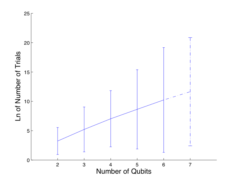
Section V.3 suggests that pure states do not require expensive MLE techniques for tomography. Nonetheless, it is interesting to see how MLE scales in runtime compared to Quick and Dirty and “Forced Purity” routines. Here we present runtimes and fidelity estimates for a pure state with and a slightly mixed state with the same tangle value which lies on the Werner state line. We also show that even the expensive MLE routine decreases in fidelity as we increase the number of qubits. For this analysis we assume that an experiment can be performed a sufficiently large number of times, to be exact.
In conclusion, “Forced Purity” results in lower Fidelity values for 2 qubits than “Quick and Dirty”, but then increases in Fidelity and converges to MLE’s fidelity for a higher number of qubits.
| n | MLE | Iteration Time | Q & D | FP |
|---|---|---|---|---|
| 2 | ||||
| 3 | ||||
| 4 | ||||
| 5 | ||||
| 6 |
| n | MLE | Iteration Time | Q & D | FP |
|---|---|---|---|---|
| 2 | ||||
| 3 | ||||
| 4 | ||||
| 5 | ||||
| 6 |


VI Conclusion
We have demonstrated that if the experiments can be performed a sufficient number of times, then using ‘‘Forced Purity” routine, tomography can be performed in a quick and robust manner. However, as the entropy of a state increases, a much more expensive MLE routine has to be used to perform tomography, which does not scale well as the number of qubits increases. Quantum computing requires only pure state tomography, for which we have obtained a scalable and efficient routine 44 4 The runtimes of the routines mentioned in this paper can be improved linearly using parallel computation. However, because the complexity increases exponentially with the number of qubits, an efficient routine to performing tomography is crucial..
Acknowledgements.
The authors would like to thank Robin Blume-Kohout, René Stock and Rob Adamson for stimulating discussions and useful comments. This work was supported by the U.S. Army Research Office, NSERC and Project OpenSource.Appendix A Matrix Differential Calculus Theorems
The following theorems were used to derive an analytic expression to the gradient
of the MLE function, which is more computationally efficient than the finite-difference gradient computation as the MLE function itself is expensive to evaluate.
If is a real-valued matrix and , then [11, 13, 12]:
| (39) |
The following are defined for real square matrices [13]:
| (40) | |||||
| (41) | |||||
| (42) | |||||
| (43) |
We begin by observing that
| (44) |
which immediately implies that
Hence, using matrix calculus, we have the result
| (45) |
Eq. (45) is a compact means of stating the result of Eq. (44) using a matrix, where the value of the derivative is stored in the original position of in the Cholesky-decomposed matrix . This is the general idea behind all matrix calculus results we have used. We could have also obtained the same result by applying matrix calculus directly. For example, denote
Then using Eq. (40) and Eq. (41)
and
This is consistent with our result in Eq. (45).
Next, we set out to compute . Recall that , hence,
References
- [1] U. Leonhardt, Measuring the quantum state of light (Cambridge University Press, 1997).
- [2] M. G. A. Paris and J. Řeháček (eds.), Quantum State Estimation, Lecture Notes in Physics 649 (Springer, Heidelberg, 2004).
- [3] M. Hayashi (ed.), Asymptotic Theory of Quantum Statistical Inference: Selected Papers (World Scientific, Singapore, 2005).
- [4] D. F. V. James, P. G. Kwiat, W. J. Munro, and A. G. White, Phys. Rev. A 64, 052312 (2001).
- [5] H. Häffner, W. Hansel, C. F. Roos, J. Benhelm, D. Chek-al-kar, M. Chwalla, T. Körber, U. D. Rapol, M. Riebe, P. O. Schmidt, C. Becher, O. Gühne, E. Dür, and R. Blatt, Nature (London) 438, 643 (2005).
- [6] H. Häffner, private communication.
- [7] See, for example, C. Cohen-Tannoudji, B. Diu and F. Laloë, Quantum Mechanics (John Wiley: New York, 1977), Complement DIII.
- [8] We assume the standard form for the Pauli matrices, with ; see, for example, C. Cohen-Tannoudji, et al., op. cit., Complement AIV. The matrix is the two-dimentional identity operator.
- [9] W. H. Press, Numerical recipes in C: The art of scientific computing ed., (Cambridge University Press, 1992).
- [10] Michael T. Heath, Scientific Computing: An Introductory Survey, Edition (McGraw Hill, Toronto, 2002).
- [11] J. R. Magnus and H. Neudecker, Matrix Differential Calculus with Applications in Statistics and Economics (John Wiley and Sons Ltd., Toronto, 1988).
- [12] D. A. Turkington, Matrix Calculus & Zero-One Matrices (Cambridge University Press, New York, 2002).
- [13] A. Graham, Kronecker Products and Matrix Calculus: With Applications (Halsted Press, Toronto, 1981).
- [14] We thank to all the users of Matlab File Exchange whose codes we have used to produce better graphics for the plots in this paper.
- [15] R. L. Kosut, A. Shabani, and D.A. Lidar, Phys. Rev. Lett. 100, 020502 (2008).
- [16] R. L. Kosut, I. Walmsley, and H. Rabitz, arXiv:quant-ph/0411093 (2004).
- [17] W. K. Wootters, Phys. Rev. Lett. 80, 2245 (1998).
- [18] A. Wong and N. Christensen, Phys. Rev. A 63, 044301 (2001).
- [19] R. Jozsa, J. Mod. Opt. 41, 2315 (1994).
- [20] GNU Scientific Library, http://www. gnu. org/ software/ gsl/ .