Improved constrained scheme for the Einstein equations: An approach to the uniqueness issue
Abstract
Uniqueness problems in the elliptic sector of constrained formulations of Einstein equations have a dramatic effect on the physical validity of some numerical solutions, for instance, when calculating the spacetime of very compact stars or nascent black holes. The fully constrained formulation (FCF) proposed by Bonazzola, Gourgoulhon, Grandclément, and Novak is one of these formulations. It contains, as a particular case, the approximation of the conformal flatness condition (CFC) which, in the last ten years, has been used in many astrophysical applications. The elliptic part of the FCF basically shares the same differential operators as the elliptic equations in CFC scheme. We present here a reformulation of the elliptic sector of CFC that has the fundamental property of overcoming the local uniqueness problems. The correct behavior of our new formulation is confirmed by means of a battery of numerical simulations. Finally, we extend these ideas to FCF, complementing the mathematical analysis carried out in previous studies.
pacs
04.20.Ex, 04.25.Nx, 04.25.D-, 97.60.-sI Introduction
In recent years we have seen the successful application of numerical codes to accurately calculate the spacetimes of compact astrophysical objects like collapsing stellar cores, (proto)neutron stars, and black holes. Most of these codes are based on the formalism of general relativity (see, e.g., [1, 2, 3] for reviews). They typically fall into two classes. One approach relies on the free evolution of the Einstein equations, recast in order to cure long-term stability problems. Here the constraint equations are only solved initially, and closely monitored at each time step to control the accuracy of the numerical solution.
Alternatively, formulations based on a constrained evolution, where the constraints are solved in parallel with evolution equations, have proven to be successful as well. Such approaches exhibit the advantage that the solution cannot violate the constraints by definition (within the accuracy of the numerical scheme). In particular, the conformally flat approximation [4, 5] (hereafter CFC) of the full Einstein equations, which constitutes a fully constrained formulation, has been shown to yield long-term stable evolutions of such astrophysical scenarios (see, e.g., [6, 7, 8, 9]). However, apart from computational challenges, arising from the need to frequently solve the elliptic constraint equations, constrained formulations suffer from mathematical nonuniqueness problems when the configuration becomes too compact. In the case of the collapse of a stellar core or a (proto)neutron star to a black hole, such a situation is encountered already before the apparent horizon forms. This issue has, in the past, been prohibitive to successfully applying such formulations in numerical simulations of a wide range of astrophysical problems.
The nonuniqueness of solutions stems from the non-linearity of the constraint equations and has been studied within the so-called extended conformal thin sandwich (XCTS) [10, 11, 12] approach to the initial data problem in general relativity. In Ref. [13] a parabolic branching was numerically found in the solutions to the XCTS equations for perturbations of Minkowski spacetime, providing the first evidence of nonuniqueness in this elliptic system. First analytical studies have been carried out in [14, 15], finding support for the genericity of this nonuniqueness behavior. More specifically, the XCTS elliptic system is formed by the Einstein constraint equations in a conformal thin sandwich (CTS) decomposition [10] supplemented with an additional elliptic equation for the lapse function, which follows from the maximal slicing condition. Although no general results on existence and uniqueness for the XCTS system are available (in contrast to the CTS case and similar elliptic systems encompassing only the constraints; see, e.g., [16, 17, 1, 10, 11]), the analysis in [14] strongly suggests the presence of a wrong sign in a certain term of the lapse equation as the culprit for the loss of uniqueness, essentially because it spoils the application of a maximum principle to guarantee uniqueness. Moreover, in these circumstances (namely, the existence of a nontrivial kernel for the XCTS elliptic operator) it is shown in [15] that the parabolic behavior found in [13] is indeed generic.
Certain constrained evolution formalisms which incorporate elliptic gauges in their schemes contain elliptic subsystems which share essential points with the XCTS equations. Nonuniqueness in the elliptic subsystem is certainly an issue for the well-posedness of the whole elliptic-hyperbolic evolution system. In numerical implementations this can depend on the employed numerical scheme, in particular, on its capability to remain close to one of the solutions, at least as long as the solution stays sufficiently far from the branching point. In fact, constrained or partially constrained evolutions have shown to be robust in a variety of contexts (see, e.g., the references in [18] and Sec. 5.2.2 of [19]). However, the problems described above have also emerged, for instance, in the axisymmetric case in [20, 21] (see also [22]). The analysis in [18] concludes that the reason behind the failures in these axisymmetric formulations is in fact related to the presence of wrong signs or, more precisely, to the indefinite character of certain non-linear Helmholtz-like equations present in the scheme (see [18] for details and also for a parallel numerical discussion in terms of a class of relaxation methods for the convergence of the elliptic solvers). Regarding the full three-dimensional case, fully constrained formalisms have been presented in [23, 25, 24]. While the work in [23, 24] includes an elliptic subsystem closely related to the XCTS equations and therefore suffers potentially from these nonuniqueness problems, the uniqueness properties of the scheme of [25] must yet be studied. In both cases, the full numerical performance still has to be assessed.
The goal of the present work is to discuss a scheme addressing the nonuniqueness issues of XCTS-like elliptic systems in the full three-dimensional case, with astrophysical applications as our main motivation. Having the analysis of the fully constrained formalism (hereafter FCF) of [23, 24] as our ultimate aim, we focus on an approximation in the spirit of the CFC approximation by Isenberg, Wilson, and Mathews [4, 26]. This methodological choice is justified since the CFC scheme already contains the relevant elliptic system of FCF, but in a setting in which potential additional problematic issues related to the FCF hyperbolic part do not mix up with the specific problem we are addressing here. Therefore, we discuss in detail a modification of the CFC scheme (in the presence of matter) where maximum-principle lines of reasoning can be used to infer the uniqueness of the solutions. We investigate numerically the performance of the new CFC scheme and finally indicate the main lines for its generalization to the full Einstein FCF case.
The article is organized as follows. In Sec. II we review the FCF and CFC formalisms, and then discuss the limitations found in the numerical implementations of the latter. In Sec. III we introduce the modification of the CFC scheme, with the aim of solving the uniqueness issues, and we present various numerical tests of the new scheme in Sec. IV. In Sec. V the guidelines for the generalization to the FCF case are discussed, and conclusions are drawn in Sec. VI. In the Appendix we justify a further approximation assumed in Sec. III which is consistent with the CFC setting. Throughout the paper we use the signature for the spacetime metric, and units in which . Greek indices run from 0 to 3, whereas Latin ones from 1 to 3 only.
II The fully constrained formalism and the conformal flatness condition
II.1 A brief review of the fully constrained formalism
Given an asymptotically flat spacetime we consider a splitting by spacelike hypersurfaces , denoting timelike unit normals to by . The data on each spacelike hypersurface are given by the pair , where is the Riemannian metric induced on . We choose the convention for the extrinsic curvature. With the lapse function and the shift vector , the Lorentzian metric can be expressed in coordinates as
| (1) |
On the other hand, we can write
| (2) |
where is the Levi–Civita connection associated with and represents the Lie derivative with respect to the evolution vector . As in [23] we introduce a time independent flat metric , which satisfies and coincides with at spatial infinity. We define and . This fiducial metric permits the use of tensor quantities rather than tensor densities. The next step in the formulation of [23] is the conformal decomposition of the fields. First, a representative in the conformal class of is chosen, so we can write
| (3) |
where and , and . In Ref. [23], the choice was adopted, leading to the following expression of in terms of the lapse and shift :
| (4) |
being the Levi–Civita connection associated with . This is in the spirit of the decomposition employed in the (X)CTS approach to initial data. Regarding the choice of the representative of the conformal metric , a unimodular condition was adopted in [23], so that . The deviation of the conformal metric from the flat fiducial metric is denoted by , i.e.
| (5) |
Once the conformal decomposition is performed, a choice of gauge is needed in order to properly reformulate the Einstein equations as partial differential equations. The prescriptions in [23] are maximal slicing and the so-called generalized Dirac gauge,
| (6) |
where stands for the Levi–Civita connection associated with the flat metric . The Einstein equations then become a coupled elliptic-hyperbolic system to be solved for the basic variables , , , and [23].
Expressing the differential operators in terms of the connection of the flat metric, the elliptic part can be written as
| (7) | |||||
| (8) | |||||
| (9) | |||||
where stands for the flat Laplacian (), , and are, respectively, the energy density, momentum density, and trace of the stress tensor, all measured by the observer of 4-velocity (Eulerian observer): in terms of the energy-momentum tensor , , , and , with . Furthermore,
| (10) | |||||
| (11) | |||||
| (12) |
Equation (7) follows from the Hamiltonian constraint, whereas Eq. (9) results from the momentum constraint together with the preservation of the Dirac gauge in time. Equation (8) corresponds to the preservation in time of the maximal slicing condition, . Note that expression (10) for the Ricci scalar of the conformal metric does not involve any second order derivative of the metric; this property follows from Dirac gauge [23]. The resulting elliptic subsystem coincides with the XCTS system [11], except from the field chosen to solve the maximal slicing equation: Eq. (8) above is to be solved for , whereas in [11] the conformal lapse is employed instead. This directly affects the value (and, in particular, the sign) of the power of the conformal factor in the nonlinear terms of Eqs. (7) and (8). More generally, one could define a generic rescaling of the lapse, , such that the choice in [11] corresponds to , whereas the choice in Eq. (8) above corresponds to (see [27] for the general equations in the vacuum case). An important remark is the absence of a choice of such that the factors multiplying and on the right hand side of the linearized versions of Eqs. (7) and (8) both present a positive sign. In the presence of matter, terms multiplying the energy density also contribute to these sign difficulties, though in this case they can be fixed by an appropriate conformal rescaling of the energy density (see later). An additional concern in a generic evolution scenario is the sign of , which is also relevant in the linearized equations. Implications of this issue are discussed in Sec. III.
The Einstein equations in the form of the elliptic equations (7)-(9) and the hyperbolic equation for as given in Ref. [23] are to be solved together with the hydrodynamic equations,
| (13) | |||||
| (14) |
where is the Levi–Civita connection associated with the metric , is the rest-mass (baryon mass) density, and is the 4-velocity of the fluid.
II.2 The conformal flatness approximation
If the hyperbolic part of the FCF system is not solved, but rather the condition is imposed, the resulting three-metric is conformally flat, and the CFC approximation is recovered. Therefore, the FCF is a natural generalization of the CFC approximation. The latter has been used in many astrophysical applications, like the rotational collapse of cores of massive stars [6, 28, 29, 30] or supermassive stars [8], the phase-transition-induced collapse of rotating neutron stars to hybrid quark stars [9], equilibrium models of rotating neutron stars [31, 32], as well as for binary neutron star merger [26, 7, 33, 34]. The elliptic subsystem of the FCF, Eqs. (7)–(9), reduces in CFC to
| (15) | |||||
| (16) | |||||
| (17) |
where the following rescaled matter quantities have been introduced, following York [1]:
| (18) | |||||
| (19) | |||||
| (20) |
Equations (15) and (16) inherit the local nonuniqueness problems already present in the FCF equations. Although the sign problems specifically related to the energy density terms are solved by the conformal rescaling of the components of the energy-momentum tensor and the CFC eliminates the term, problems related to the term remain in the scalar CFC equations. This is apparent once the extrinsic curvature is expressed in terms of the lapse and the shift.
Conformal rescaling of the hydrodynamical variables is not only relevant for local uniqueness issues. The hydrodynamic equations (13) and (14) can be formulated as a first-order hyperbolic system of conservation equations for the quantities [35, 36], where, similarly to Eqs. (18)–(20), , being the baryon mass density as measured by the Eulerian observer. We can thus consider and as known variables in the computation of the CFC metric. Note that these quantities differ from and by a factor , and hence it is not possible to compute the nonstarred quantities before knowing the value of . If the energy-momentum tensor represents a fluid, then the source of Eq. (16) cannot be explicitly expressed in terms of , the reason for that being the dependence of on the pressure . The pressure can only be computed in terms of the “primitive” quantities, e.g., as a function of the rest-mass density and the specific internal energy . The primitive quantities are, in general, recovered from implicitly by means of an iteration algorithm. So far, two solutions of the problem related to the fact that directly contains have been used in numerical simulations performed with the CFC approximation.
The first approach [26] is to consider , and hence also , as an implicit function of . Then Eqs. (15)–(17) can be solved as a coupled set of nonlinear equations using a fixed-point iteration algorithm. The convergence of the algorithm to the correct solution depends not only on the proximity of the initial seed metric to the solution, but also on the uniqueness of this solution. The latter point is extensively discussed in Sec. III. Furthermore, one problem of this approach is the necessity of performing the recovery of the primitive variables (which is numerically a time consuming procedure) to compute the pressure during each fixed point iteration. Because of the uniqueness problem, this approach can be only successfully applied in numerical simulations for, at most, moderately strong gravity (like stellar core collapse to a neutron star or the inspiral and initial merger phase of binary neutron stars), but fails for more compact configurations like the collapse of a stellar core or a neutron star to a black hole. For such scenarios with very strong gravity, one finds convergence of the metric to a physically incorrect solution of the equations or even nonconvergence of the algorithm.
A second approach to the recovery algorithm problem is the attempt to calculate independently of the CFC equations. This can be achieved by computing the conformal factor by means of the evolution equation
| (21) |
The conformal factor obtained in this way is analytically identical to the from Eqs. (15)–(17), but here we use a different notation to keep track of the way it is computed. The value of is solely used to evaluate , and the coupled system of Eqs. (15)–(17) is solved for determining , , and . Although this approach allows one to avoid the problem of recovering the primitive variables at each iteration, it also suffers from the convergence problem, and the simulation of configurations with very strong gravity is still not feasible. Furthermore, new complications are introduced by using two differently computed values, and , of the same quantity. For some scenarios like the formation of a black hole from stellar collapse, the numerical values of these two quantities during the evolution of the system start to diverge significantly at some point. We find that this inconsistency cannot be avoided, since any attempt to artificially synchronize both values leads to numerical instabilities.
III The new scheme in the conformally flat case
III.1 Uniqueness of the elliptic equations and convergence of elliptic solvers
Well-posed elliptic partial differential systems admit non-unique solutions whenever the associated differential operator has a nontrivial kernel. When discussing sufficient conditions guaranteeing uniqueness, it is illustrative to first consider the case of a scalar elliptic equation. In particular, for the class of scalar elliptic equations for the function of the form
| (22) |
where and are known functions independent of , a maximum principle can be used to prove local uniqueness of the solutions as long as the sign of the exponent is different from the sign of the proper function [39, 1, 37, 38].
In the CFC case, we are not dealing with a single scalar elliptic equation, but rather with the coupled non-linear elliptic system (15)-(17). Therefore, assessing wheter or not the scalar equations (15) and (16) present the good signs for the application of a maximum principle is an important step for understanding the uniqueness properties of the whole system. However, as pointed out in the previous section, the CFC equations for the conformal factor and the lapse possess the wrong signs in the quadratic extrinsic curvature terms (once everything is expressed in terms of the lapse and the shift). This problem can be fixed in Eq. (15) by an appropriate rescaling of the lapse, , but this strategy does not solve the problem for the lapse equation (cf. the discussion on the conformal lapse in Sec. II.1). Therefore, we cannot use the maximum principle to infer local uniqueness of the solutions to the CFC equations. In these conditions of potential nonunique solutions, convergence to a undesirable solution may happen. As mentioned in the introduction, this pathology has been illustrated using simple analytical examples of scalar equations of the type (22) in [14], as well as in numerical implementations of the vacuum Einstein constraints in the XCTS approach [13] and certain constrained evolution formalisms (see, e.g., [18]).
In the context of the CFC approximation this sign issue has also appeared, in particular associated with the “recovery algorithm” problem discussed in Sec. II.2 since it involves the evaluation of the conformal factor. Nonunique solutions of , either due to the use of the nonconformally rescaled or the quadratic extrinsic curvature term, spoil the convergence of the algorithm when density, and thus compactness, increases. We again emphasize that a possible synchronization of and does not solve the problem in general, since numerical instabilities eventually arise at sufficiently high compactness.
III.2 Numerical examples
The nonuniqueness of solutions has also been observed in FCF, as described in the following example. Let us consider a vacuum spacetime, with initial data formed by a Gaussian wave packet, as in [23], but with much higher amplitude instead of in [23] (see the latter reference for notations). The integration technique and numerical settings are the same as in [23], but contrary to the results for small amplitudes obtained in that reference, the wave packet does not disperse to infinity and instead starts to collapse. Fig. 1 displays the time evolution of the central lapse at and of the system’s Arnowitt-Deser-Misner (ADM) mass , which in the present conformal decomposition can be expressed as
| (23) | |||||
where the integral is taken over a sphere of radius and the second equality follows from the use of Dirac gauge [Eq. (6)].


The very sudden change at in both the central lapse and the ADM mass, which is also present in, e.g., the central conformal factor , originates from the convergence of the elliptic system (7)-(9) to another solution with a different (unphysical) value of the ADM mass. The good conservation of and the smooth evolution of for indicate that this other solution remains stable until , when high-frequency oscillations appear. These oscillations may be due to the overall inconsistency of the system, destabilizing the whole scheme. On the other hand, the time evolution of does not show any such type of behavior, and exhibits a continuous radial profile at all times. This is numerical evidence that, also for the full Einstein case (i.e. without approximation), the generalized elliptic equations suffer from a similar convergence problem as in the CFC case.
The same subject is also exemplified when one tries to calculate the spacetime metric for an equilibrium neutron star model from the unstable branch using either Eqs. (7)–(9) in the FCF case or Eqs. (15)–(17) in the CFC approximation. Even for the simple setup of a polytrope with adiabatic index in spherical symmetry, those metric equations yield – when converging at all – a grossly incorrect solution if the matter quantities in the source terms are held fixed. Both the metric components as well as the ADM mass can deviate from the physical solution by a few tens of percent, even though that incorrect metric satisfies the asymptotic flatness condition. The reason why programs for constructing rotating relativistic neutron star models, like the KEH code [40], the RNS code [41], or the BGSM code [42], are not obstructed by this nonuniqueness problem is apparently that they all utilize an iteration over both the metric and the hydrodynamic equations simultaneously, thereby allowing the matter quantities to change during the calculation of the metric.
We want to stress here that these non-convergence issues in the CFC case are not related to the approximation that is made. If one considers this system in the spherical (one-dimensional) case, CFC is no longer an approximation, but is the choice of the so-called isotropic gauge. Even then, the elliptic system (15)-(17) no longer converges to the proper (physical) solution.
III.3 The new scheme and its theoretical properties
Despite the above mentioned convergence problems, numerically simulating the physical problem of spherical collapse to a black hole in isotropic coordinates has been successfully studied by Shapiro and Teukolsky in [43]. Because of the spherical symmetry, there exists only one independent component of the extrinsic curvature. It is then possible to compute directly a conformal extrinsic curvature, , from the conserved hydrodynamical variables. The elliptic equation for then decouples from the other elliptic equations by introducing this conformal extrinsic curvature and using the conserved hydrodynamical variables in the source. This source term presents no problem for proving local uniqueness, and the equation for always converges to the physically correct solution. Once the conformal factor, the extrinsic curvature (from the conformal factor and the conformal extrinsic curvature), and the conserved hydrodynamical variables are known, the elliptic equation for can be solved and, again, the source exhibits no local uniqueness problem. This follows from the fact that the extrinsic curvature is not expressed in terms of the lapse and the shift. This contrasts with the CFC equation (16) where a division by occurs in the last term when the extrinsic curvature is expressed in terms of its constituents , , and . In addition, there is no need to use . Finally, the elliptic equation for the shift vector can be solved. In summary, no problems of instabilities or divergence are encountered.
We now generalize this scheme to the CFC case in three dimensions. This involves the use of two different conformal decompositions of the extrinsic curvature: first, two different conformal rescaling and, second, two different decompositions of the traceless part into longitudinal and transverse parts. Adopting maximal slicing, , a generic conformal decomposition can be written as
| (24) |
where is a free parameter and a free function, is transverse traceless and in the conformal Killing operator defined by Eq. (11). We implicitly make use of a flat conformal metric, with respect to which is transverse, although, in principle, it would be more general to use the metric and the conformal Killing operator associated with it, . But such a decomposition would introduce many technical difficulties in our treatment. In particular, it is numerically easier to handle tensors which are divergence-free with respect to the flat metric in the generalization to FCF. The vector , on which is acting, is therefore called the longitudinal part of . The first decomposition we use is the one introduced in Eqs. (3) and (4) with the choice and . This corresponds to a CTS-like decomposition of the traceless part, so that is given by the shift vector and can be expressed in terms of the time derivative of the conformal metric. We denote this traceless part as . In the CFC approximation this becomes
| (25) |
The second conformal decomposition,
| (26) |
refers to and . It instead corresponds to a conformal transverse traceless (CTT) decomposition of the traceless part of extrinsic curvature introduced by Lichnerowicz [44]. Notice that we have defined , not to be confused with . The relation between and is given by
| (27) |
In terms of , the CFC momentum constraint can be written as
| (28) |
Consistency between the CTT-like decomposition (26) and the CTS-like one (25) generically requires a nonvanishing tranverse part in Eq. (26). However, as it is shown in the Appendix, this is smaller in amplitude than the nonconformal part of the spatial metric and can be approximated on the CFC approximation level as
| (29) |
From Eqs. (26) and (28), an elliptic equation for the vector can be derived,
| (30) |
from which can be obtained. With this vector field, one can calculate the tensor via (29). Notice that in the case of spherical symmetry, is the quantity used by Shapiro and Teukolsky [43].
The elliptic equation for the conformal factor can be rewritten in terms of the conserved hydrodynamical variables and :
| (31) |
This equation can be solved in order to obtain the conformal factor. Once the conformal factor is known, the procedure to implicitly recover the primitive variables from the conserved ones is possible, the pressure can be computed using the equation of state, and therefore is at hand. The elliptic equation for can be reformulated by means of the conserved hydrodynamical variables, , and the conformal factor:
| (32) |
From this equation can then be obtained and, consequently, so can the lapse function . Note that, since is already known at this step, no division by spoils the good sign for the maximum principle.
Using the relation between the two conformal decompositions of the extrinsic curvature, , Eq. (25) can be expressed as . Taking the divergence, we arrive at an elliptic equation for the shift vector,
| (33) |
where the source is completely known. This elliptic equation can be solved in order to obtain the shift vector consistent with , as required by the CFC approximation.
In this recast of the CFC equations, an extra elliptic vectorial equation for the vector field is introduced. However, now the signs of the exponents of and are compatible with the maximum principle for scalar elliptic equations, and the problem is linearization stable. While this does not guarantee global uniqueness of the solutions, it provides a sufficient result for local uniqueness. This strongly relies on the fact that the system decouples in a hierarchical way, which we summarize here once more:
- 1.
With the hydrodynamical conserved quantities at hand, solve Eq. (30) for , and thus for .
- 2.
Solve Eq. (31) for , where local uniqueness is now guaranteed. Then can be calculated consistently.
- 3.
Solve Eq. (32) for , a linear equation where the maximum principle can be applied and uniqueness and existence follow with appropriate boundary conditions.
- 4.
As the source of Eq. (33) is then fully known, solve it for .
Note that this scheme is similar to that used by Shibata and Uryū [45] to compute initial data for black hole - neutron star binaries. We will discuss this point further in Sec. VI.2.
The new CFC metric equations presented here not only allow us to evolve the hydrodynamical equations and recover the metric variables from the elliptic equations in a consistent way (no auxiliary quantity is needed), but they also permit to introduce initial perturbations in the hydrodynamical variables (strictly speaking, in the conserved quantities) in a set of previously calculated initial data and directly delivers the correct values for the metric. It is even possible to perturb only the primitive quantities, and consistently resolve for the metric by iterating until the conformal factor , which links the primitive to the conserved quantities, converges. We find that such an iteration method fails for sufficiently strong gravity if the original CFC formulation is used.
IV Numerical results
We recapitulate that the original CFC formulation exhibits serious convergence problems when dealing with highly compact configurations such as nascent black holes. This weakness of the original formalism is noticeable in the fact that no simulations of rotational collapse to a black hole substantially beyond the formation of the apparent horizon have been performed so far in the CFC. Furthermore, some scenarios which do not involve the formation of a black hole are alredy feasible with the old formulation only if procedures like using Eq. (21), with all associated problems and inconsistencies, are employed. An example is the migration of a neutron star model from the stable to the unstable branch, which is a standard test for relativistic hydrodynamics codes. In contrast, the new CFC scheme presented in this work solves all problems that prevented performing such simulations in the past. In order to show the suitability of the new scheme we present the results of numerical simulations of the migration test and of the rotational collapse to a black hole.
IV.1 Model setup
The numerical simulations presented here are performed using the numerical code CoCoNuT [46, 28]. This code solves the evolution of the hydrodynamics equations coupled to the elliptic equations for the spacetime metric in the CFC approximation. Standard high-resolution shock-capturing schemes are used in the hydrodynamic evolution, while spectral methods are employed to solve the metric equations. The code is based on spherical polar coordinates, and for the tests presented here we assume axisymmetry and symmetry with respect to the equatorial plane. Note that the metric equations presented in this paper are covariant. Thus the formalism can be used for any coordinate basis as well as without any symmetry conditions.
The initial models are general relativistic polytropes in equilibrium with a polytropic constant . The models are chosen to be situated on the unstable branch, i.e. , where is the central rest-mass density. Therefore, any perturbation of the star induces either the collapse to a black hole or migration to a configuration of the same baryon mass on the stable branch. Table 1 shows the main features of these initial models. Models D1 to D4 are uniformly rotating models which are identical to those presented in [47]. The model labeled SU is a spherical model, while model labeled SS is the counterpart model with the same baryon mass but it is located on the stable branch. The equilibrium rotating star models in Dirac gauge (the axisymmetric and stationary limit of FCF) used here are described in [48], and are computed using the Lorene [49] library. We map the hydrodynamic and metric quantities to the CFC code neglecting the terms, which are negligible due to their smallness. Alternatively, we compute CFC equilibrium initial models. In this case we find that the differences with respect to the FCF models are small () for representative metric and hydrodynamic quantities, initially and during the evolution, and therefore we discuss only the FCF initial models here.
| Model | ||||||
|---|---|---|---|---|---|---|
| [] | [] | |||||
| SU | 8.000 | 0 | 1.00 | 4.267 | 1.447 | 0 |
| SS | 1.346 | 0 | 1.00 | 7.999 | 1.424 | 0 |
| D1 | 3.280 | 1.73 | 0.95 | 5.947 | 1.665 | 0.207 |
| D2 | 3.189 | 2.88 | 0.85 | 6.336 | 1.727 | 0.362 |
| D3 | 3.134 | 3.55 | 0.75 | 6.839 | 1.796 | 0.468 |
| D4 | 3.116 | 3.95 | 0.65 | 7.611 | 1.859 | 0.542 |
The hydrodynamic equation are discretized on the finite difference grid with grid points. The radial grid size is for the innermost cell and increases geometrically outwards, while the angular grid is equidistantly spaced. The metric equations are solved on a spectral grid consisting of radial domains distributed such as to homogeneously cover the finite difference grid and a compactified exterior domain extending to radial infinity. On the spectral grid we resolve each radial domain with collocation points. The spherical model needs only one angular collocation point, while we use angular points for the rotating models.
We track the location of the apparent horizon by means of a three-dimensional spectral apparent horizon finder, described in detail and tested in [50]. The apparent horizon location is given by a function , which is decomposed into a set of spherical harmonics. The coefficients of in this basis are computed iteratively, in order to satisfy the condition that the expansion in the outgoing null direction vanishes at the apparent horizon location.
IV.2 Migration of unstable neutron stars to the stable branch
The first test we consider is the migration of a neutron star model in equilibrium from the unstable branch to the stable branch, which is a standard but still demanding test for general relativistic hydrodynamics codes, as it involves the dynamic transition between two very compact equilibrium states. This test has been performed in the past in full general relativistic simulations [51]. We start the evolution with the nonrotating equilibrium model labeled SU. Since it belongs to the unstable branch, any perturbation from exact equilibrium (which can, for instance, be caused by discretization errors) leads either to a collapse or to an expansion to a new equilibrium configuration of the same baryon mass on the stable branch. The corresponding equilibrium configuration with the same baryon mass, model SS, has smaller ADM mass than the initial system (see Table 1). Therefore, to preserve the ADM mass, the final configuration cannot be exactly the equilibrium model given by SS. The energy difference between models SU and SS should be transformed into kinetic energy, remaining in the final object in the form of pulsations.
In our case the numerical truncation error is sufficient to trigger the migration. Since the final neutron star on the stable branch is larger than the initial model (see Table 1), the outer boundary of the finite difference grid is chosen to be times the radius of the model SS. We perform two simulations on a finite difference grid with or radial cells and or , respectively. We use radial domains for the spectral grid. We evolve the system with either a polytropic or an ideal gas equation of state.


Figure 2 shows the time evolution of the central values of the rest-mass density and the lapse. As the star expands, decreases while grows until the new stable equilibrium configuration is reached. In the polytropic case, there are no physical mechanisms to damp the strong pulsations, and the final state resembles a star oscillating around the equilibrium configuration until numerical dissipation finally damps the oscillations. This can be seen in the pulsating values of rest-mass density and lapse around the value corresponding to the equilibrium model on the stable branch (solid horizontal line in Fig. 2).
In the ideal gas case, shock waves are formed at every pulsation, and they dissipate kinetic energy into thermal energy, thereby damping the oscillations. As these shocks reach the surface of the star, a small amount of mass is expelled from the star and matter is ejected outwards into the surrounding artificial low-density atmosphere until it leaves the grid across the outer numerical boundary. We approximately compute the escape velocity as , where is the Newtonian potential. This formula is not exact in general relativity, but it should by sufficiently accurate near the outer numerical boundary where gravity is weaker. We find that the shock waves leaving the computational domain exceed the escape velocity and therefore the lost mass is gravitationally unbounded. We also check that these results are not affected by changing the resolution or setting the outer boundary twice as far away. As the oscillations are damped, the shocks become weaker and the mass expelled at each oscillation is smaller. At the end of the simulation the star has lost about of its initial baryon mass, approaching a state of constant baryon mass. As a consequence, the final equilibrium configuration on the stable branch is not the model SS anymore but, rather, the corresponding model from the stable branch with lower baryon mass and central density. In Fig. 2 we plot the central rest-mass density and lapse of a series of equilibrium models on the stable branch corresponding to the baryon mass remaining in the computational domain at each time. It can be seen that these values deviate with time from model SS and fit the final state in the hydrodynamical evolution of the star.
As a by-product of this study we draw reader’s attention to the consistency (as it should be) between the amplitude and the frequency of the oscillations. The period of these oscillations is approximately of the order of the hydrodynamical characteristic time , which decreases with density like . In the polytropic case, the maxima of the oscillations in are systematically higher than in the ideal gas case. Consequently, the characteristic time is shorter than in the ideal gas case, as Fig. 2 shows. A second property worth pointing out is that the low numerical viscosity of our code is responsible for maintaining a nearly constant amplitude of the oscillations (in the polytropic case) during many characteristic times.
Our simulations are consistent with the results from a fully relativistic three-dimensional code in [51]. Similar simulations of this test, with the original, unmodified CFC scheme, lead to a completely incorrect solution with a grossly incorrect ADM mass. When running with the new improved CFC scheme, we obtain and initial values for the conformal factor and lapse of and , respectively. On the other hand, with the unmodified conventional CFC scheme, the metric solver already initially converges to a solution with (55%), (61%) and (63%), where the relative differences to the physically correct solution are given in parentheses.
As presented in [52] the migration test can be successfully simulated using the old CFC scheme, if one resorts to additionally solving the evolution equation (21) for the conformal factor (which would lead to large inconsistencies in scenarios with higher compactness but still yields acceptable results for the standard migration case). Here the superiority of the new, fully consistent CFC scheme, which does not depend on such scenario-dependend amendments, alredy becomes apparent.
IV.3 Collapse of unstable neutron stars to a black hole
As the second test we present the collapse of a (spherical or rotating) neutron star model to a black hole. Following [47] we trigger the collapse to a black hole by reducing the polytropic constant by in the initial models D1 to D4. Alternatively, in the spherical SU model we increase the rest-mass density by , which yields a similar dynamic evolution. However, since the models are initially in equilibrium, the total collapse time depends strongly on the perturbation applied. In these cases, the outer boundary of the finite difference grid is larger than the star radius. For the spherical SU model, we perform two simulations using or radial cells and or , respectively, to assess the resolution dependence of our simulations. For the rotating models D1 to D4 the grid is made up of and cells, with the same radial grid spacing as in the spherical model. We choose radial domains for the spectral grid. As in [47] we use a polytropic equation of state in the evolution.


The top panel of Fig. 3 shows the evolution of the rest-mass density and lapse at the center. Since for the maximal slicing condition the singularity cannot be reached in a finite time, rapidly approaches zero once the apparent horizon has formed. In parallel, grows, which results in a decrease of the numerical time step due to the Courant condition applied to the innermost grid cell. We terminate the evolution as the central regions of the collapsing star inside the apparent horizon become increasingly badly resolved on the regular grid, and thus numerical errors grow. We check in SU model that by refining the radial resolution we are able to follow the collapse to even higher densities. Therefore, the only limitation to perform a stable evolution after the apparent horizon formation is the numerical resolution used. Note, however, that the spatial gauge condition is fixed in CFC, and thus we are not able to utilize the common method of exploiting the gauge freedom for the radial component of the shift vector in order to effectively increase the central resolution.
In the bottom panel of Fig. 3 we display the time evolution of the apparent horizon radius. As expected, the apparent horizon appears at a finite radius and already encompasses a significant fraction of the total mass of the star () at that time. Afterwards, its radius grows as the surrounding matter falls inside beyond the horizon. The fraction of the rest mass remaining outside the horizon is also plotted in the figure. In the rotating case the apparent horizon is slightly nonspherical. The ratio of the polar to the equatorial proper circumferential radius of the apparent horizon at the end of the simulation is for models D1 to D4, where and .
Since we cannot reasonably determine the location of the event horizon, as this would require the evolution of spacetime until the black hole has become practically stationary, we utilize the apparent horizon radius to estimate the mass of the newly formed black hole. Following the prescription in [47] we use the expression . Note that this formula is only strictly valid for a stationary Kerr black hole. In our case, however, first of all, some (albeit a small) amount of matter is still outside the horizon and the black hole is still dynamically evolving, and second, the metric of a Kerr black hole is not conformally flat [53]. Still, according to [47] this approximation (excluding the effects of CFC) introduces an error in the mass estimate of only . For the spherical model the estimated value for at the end of the simulation agrees within with the ADM mass of the initial model, while in the rotating models D1 to D3 the error is . In all these cases the above formula overestimates the black hole mass. Because of its rapid rotation and the resulting strong centrifugal forces, in model D4 the collapse deviates significantly from sphericity, leading to a strongly oblate form of the density stratification. Consequently, we still find a non-negligible amount of matter outside the apparent horizon at the end of the simulation (about of the total rest mass). Therefore the value for is smaller than . In Fig. 4 we present the distribution of the rest-mass density and the location of the apparent horizon at the end of the simulation for this particular model. Since the time evolution is limited by our chosen, still computationally affordable, grid resolution in the central region, we are not able to evolve this model to times when a disk forms as in [47]. Nevertheless, all other quantities qualitatively agree with the results in that work, although we refrain from performing a more detailed comparison due to the respective differences in the gauge of the two formulations used in [47] and in this study, respectively.
In the near future we plan to carry out an exhaustive analysis of the scenario of a collapse to a black hole by comparing, on one hand, the CFC formulation with FCF (see Sec. V), and, on the other hand, the FCF with other (free evolution) formulations. The difficulties induced by the use of different gauges can be overcome by using gauge-invariant quantities for comparison and analyzing their behavior as a function of proper time.
V Generalization to the fully constrained formalism
The ideas presented in Sec. III can be generalized to the FCF approach of the full Einstein equations described in Sec. II.1.
As shown in [24], the hyperbolic part of FCF can be split into a first order system. The reformulation of the CFC equations presented in Sec. III relies on the rescaled extrinsic curvature given by Eq. (27). Consequently, we write the FCF hyperbolic part as a first order system in , instead of first order system in as in [24], arriving at
| (34) | |||||
| (35) | |||||
where
| (36) | |||
| (37) |
The system is closed by adding the equation
| (38) |
which is derived from applying partial derivatives with respect to in the definition of . Moreover, the system observes the constraint of Dirac gauge, [Eq. (6)], and for the determinant of the conformal metric, we obtain . The first order system given by Eqs. (34)–(38) has the same properties regarding hyperbolicity and existence of fluxes as the one in [24]. It has the advantage over the second order system for proposed in Ref. [23] of getting rid of partial derivatives with respect to of the lapse , the shift , or the conformal factor .
The elliptic part of FCF can be rewritten, using the tensor , as
| (39) | |||||
| (40) | |||||
| (41) |
The strategy to evolve the two symmetric tensors and relies on a decomposition of these tensors in longitudinal and transverse traceless parts. The longitudinal parts (divergences with respect to the flat metric) are either known a priori or are determined by the elliptic equations. More specifically, the divergence of vanishes according to the Dirac gauge, whereas the divergence of is determined by the momentum constraint (42) – see below. Consequently, focus is placed on the transverse traceless parts of these tensors. The latter are described in a pure-spin tensor harmonic decomposition, as discussed in a previous article [24]. In particular, each transverse traceless tensor is fully expressed in terms of two scalar potentials (named and in [24]) that are evolved according to evolution equations obtained from the transverse traceless parts of Eqs. (34) and (35) for and , respectively, by applying consistently the decomposition in [24]. Once the scalar potentials on the next time slice are determined, the tensors and can be reconstructed completely, satisfying the divergence-free conditions. This fully fixes , whereas in the case of the longitudinal part is computed in a very similar way to the CFC case, i.e. by determining the vector from the momentum constraint as described hereafter.
From Eq. (26), the momentum constraint can be written as
| (42) |
which is equivalent to the following elliptic equation for :
| (43) |
This elliptic equation for the vector is linear. Since and have been calculated previously, we can solve the elliptic equation (43) to obtain the vector . With this method, the Dirac gauge and the momentum constraint are guaranteed to be satisfied. Then, is reconstructed from and on the new time slice.
At this point, since the tensors and are known, we can follow exactly the same scheme as in the CFC case to solve in a hierarchical way the elliptic equations. First the conformal factor is obtained from Eq. (39), then the lapse function from Eq. (40), and finally the shift vector is acquired from Eq. (41). These equations are decoupled in the order mentioned. No sign problems are exhibited in the scalar elliptic equation and therefore the maximum principle can be applied. A minor concern is associated with the sign of the term in Eq. (39), but unique solutions also exist for negative conformal Ricci scalars (closely related to ). Note that, contrary to the CFC case, here no (additional) approximation has been made: it is simply a new scheme to write down FCF, where the elliptic part is better behaved from the point of view of local uniqueness. Numerical simulations with this FCF scheme will be presented in a future publication.
VI Discussion
VI.1 Summary
We have presented an approach to the solution of the uniqueness issues appearing in certain constrained formulations of Einstein equations. We have illustrated the problem and its solution through a detailed analytical and numerical study of a waveless approximation that retains all the involved essential features.
More specifically, we have reformulated XCTS-like elliptic systems appearing in constrained evolution schemes of the Einstein equations, like FCF of [23, 24], as well as in the CFC approximation [4, 5]. Such systems require the simultaneous solution of the constraints, in particular, the momentum constraint for the shift, together with a maximal slicing condition for the lapse. The resulting elliptic system presents potential local nonuniqueness problems, and numerical implementations have indeed encountered such obstacles. The original CFC formulation has not been able to cope with these problems, as it suffers from convergence of the system to unphysical solutions or nonconvergence at all in high density regimes. We have suggested that these problems are not due to the approximative nature of CFC, since FCF in the variant of [23, 24], which is a natural generalization of CFC to the nonconformally flat case, also suffers from the same problems. In order to address these issues, first focusing on the simpler CFC case, we have considered the conformal rescaling of the traceless part of the extrinsic curvature, resulting in the expression for in Eq. (27), which is a rescaling different from the respective ones employed in FCF and the CFC approximation, but coincides with the one in the XCTS approach of [10, 11]. This is motivated by the work of Shapiro and Teukolsky [43], who simulated the collapse of a neutron star model using such a reformulation of the CFC metric equations (however, restricted to spherical symmetry in their case) and apparently did not encounter any of the problems described above. Extending their approach to three dimensions, we have decomposed into longitudinal and transverse parts as in the CTT formulation of the constraint equations (29). The divergence (i.e. the longitudinal part) of this tensor is determined by the momentum constraints, Eqs. (28) in the CFC case, just as in the CTT formulation. In the CFC scheme, we have neglected the transverse part of this tensor, as the order of its error is higher than the one arising from the CFC approximation itself. In the nonapproximate FCF case, the transverse part of is determined by an evolution equation. Once the conformal extrinsic curvature is obtained, it can be employed in the Hamiltonian equation to calculate the conformal factor . The lapse is then fixed through the maximal slicing condition, and the resulting equation allows the application of a maximum principle uniqueness argument. Finally, the shift is found through the kinematical relationship defining the extrinsic curvature, leading to Eq. (33).
By performing a variety of tests, we have provided evidence that the problem of convergence to an unphysical solution of the metric equations (or even complete nonconvergence) in the original formulation of the CFC scheme is fully cured by our new reformulation. Not only can numerical results in the original CFC scheme (in the, at most, moderately gravitationally compact regime where that system still yields physically correct solutions) be reproduced by the new formulation but, more importantly, the new numerical results presented here exhibit the proper numerical and physical behavior even for highly compact configurations. For the first time, it has been possible to successfully perform both the migration test and the collapse of a neutron star to a black hole in the CFC case in a consistent way. Our new formulation thus facilitates simulations in the high density regime of those scenarios where the CFC is still a reasonably fair approximation, that is, for systems which are not too far from sphericity, like stellar gravitational collapse.
VI.2 Comparison with previous works
As compared to the original CFC formulation by Isenberg [4] and Mathews and Wilson [5], the scheme presented here is augmented by an additional vector elliptic equation for , while the elliptic character of the system of metric equations is preserved. The new scheme reformulates the CFC approximation in a CTT shape (one scalar and one vector elliptic equation), and then solves for the lapse and the shift (one additional scalar and one vector elliptic equation). In contrast, the original CFC scheme employed an (X)CTS approach where, together with two scalar elliptic equations, only one vector elliptic equation was present. In contrast to the original scheme, the elliptic system in the new formulation not only corrects the problem of local uniqueness in the scalar elliptic equations, but also introduces a hierarchical structure that decouples the system in one direction.
In the context of the conformally flat approximation, the same “augmented CFC” scheme as that discussed here has been introduced already by Saijo [8] to compute gravitational collapse of differentially rotating supermassive stars. However, in this work the inconsistency between Eq. (25) and Eq. (29), i.e. setting to zero the transverse traceless part of , has not been pointed out. On the contrary, we have analyzed this inconsistency in detail (cf. the Appendix) and have shown that it leads to an error of the same order as that of the CFC approximation. In addition, we have shown here that the introduction of the vector potential is the key ingredient for solving the nonuniqueness issue.
The same scheme, but without the conformal rescaling of the matter quantities, has also been used recently by Shibata and Uryū [45] in the context of computing initial data. As in [8], the inconsistency resulting from setting to zero the transverse traceless part of and the uniqueness issue are not discussed in their work. We emphasize that the these studies [8, 45] do not discuss the extension of the new scheme to the nonconformally flat case, as done here.
Let us also mention that the augmented CFC scheme presented here can be regarded as a hybrid mixture of some of the waveless approximation theories (WAT) proposed by Isenberg [4]. In fact, the CFC approximation using the two choices and [as employed in Eq. (33)] corresponds to version WAT-I. On the other hand, the approximation used in Eq. (29) is in the spirit of the vanishing transverse traceless part of the extrinsic curvature in the (coupled) version, WAT-II (although WAT-II refers to the physical extrinsic curvature, whereas here we have dealt with the conformal one). As mentioned above, both assumptions are consistent at the considered level of approximation, as shown in the Appendix.
Regarding the complete constrained evolution of the Einstein equations, we have generalized the ideas presented here for the CFC case to the elliptic part of FCF. In previous studies [23, 24], the hyperbolic part of Einstein equations resulted in a wave-type equation for the tensor , representing the deviation of the three-metric from conformal flatness. With the introduction of we have recovered here a first-order evolution system, analogous to the standard Hamiltonian system, in which we have, however, retained only the divergence-free terms. Thus, for both and , the transverse (divergence-free) parts are evolved by this system, while the longitudinal parts are fixed either by the gauge (for ), or by the momentum constraint (for ). Numerical results for this case will be presented in future studies.
We finally comment on the recent work by Rinne [18], where uniqueness problems appearing in certain constrained and partially constrained schemes for vacuum axisymmetric Einstein equations [20, 54] are addressed. As in the present case, uniqueness issues related to the Hamiltonian constraint equation are solved by adopting an appropriate rescaling the extrinsic curvature. On the other hand, problems associated with the slicing condition are tracked to the substitution in that equation of the extrinsic curvature by its kinematical expression in terms of the (shift and the) lapse. The latter spoils the uniqueness properties by reversing the sign of the relevant term in the slicing equation. This problem is solved by enlarging the elliptic system with an additional vector so as to reexpress the relevant components of the extrinsic curvature without resorting to the lapse. The resulting elliptic system also presents a hierarchical structure. Although the spirit of such approach is close to the one here presented, the specific manner of introducing the additional vector variable in [18] critically relies on the two dimensionality of the axisymmetric problem (specifically, on a choice of a particular gauge and on the fact that vectors and rank-two traceless symmetric tensors have the same number components in two dimensions, a property lost in three dimensions). On the contrary, the introduction of the vector through the CTT decomposition (29) is properly devised to work in three dimensions. Relevant related discussions in the three-dimensional context can be found in Sec. 3.4 of [18] (where the relation between nonuniqueness problems in XCTS and axisymmetric constrained evolution schemes is discussed) and in the three-dimensional constrained evolution scheme presented by Moncrief et al. in [25].
Acknowledgements.
It is a pleasure to thank J. M. Ibáñez, M. Saijo and K. Uryū for many fruitful discussions. I. C.-C. acknowledges support from from the Spanish Ministerio de Educación y Ciencia (AP2005-2857), and H. D. is supported by the Marie Curie Intra-European Fellowship within the 6th European Community Framework Programme (IEF 040464). This work was supported by the Ministerio de Educación y Ciencia through Grant No. AYA2007-67626-C03-01, by the Deutsche Forschungsgemeinschaft through the Transregional Collaborative Research Center Grant No. SFB/TR 7 “Gravitational Wave Astronomy”, by the French ANR Grant No. 06-2-134423 “Méthodes mathématiques pour la relativité générale”, by the French–Spanish bilateral research Grant No. HF2005-0115, and by the European Network of Theoretical Astroparticle Physics ENTApP ILIAS/N6 under Contract No. RII3-CT-2004-506222.Appendix A Consistency of the approximation
In the derivation of the new formalism we make use of the fact that in CFC. We show next that this assumption is completely consistent at the accuracy level of the CFC approximation. In the first place, we need to estimate the error of the CFC approximation itself. By definition, the CFC three-metric deviates linearly with from the (exact) FCF case. It can be easily shown from the FCF equations (39)-(41) that the metric quantities behave as
| (44) | |||||
| (45) | |||||
| (46) |
Therefore can be used as an estimator for the error of the CFC approximation.
Two limits in which CFC is exact will be considered. First, in spherical symmetry the CFC metric system is an exact reformulation of the Einstein equations since in the FCF metric. If the system is close to spherical symmetry (i.e. spheroidal), and if we are able to define a quasispherical surface of the system (e.g., the surface of a star or the apparent horizon of a black hole), then the equatorial and polar circumferential proper radius, and , can be computed, and we can define the ellipticity of the system as
| (47) |
Close to sphericity, scales linearly with , and we can ensure that the error of CFC is . The second limit to consider is if a post-Newtonian expansion of the gravitational sources is possible, i.e. if the post-Newtonian parameter , where , , and are the typical velocity, mass, and length of the system, respectively. In this case the CFC metric behaves like the first post-Newtonian approximation [56, 55], i.e.
| (48) | |||||
| (49) | |||||
| (50) |
Note that, for clarity, we explicitly retain powers of the speed of light as factors in the equations throughout this appendix. In the case that both limits are valid, i.e. close to sphericity and in the post-Newtonian expansion, the nonconformally-flat part of the three-metric behaves like . The next step is to compute the behavior of the CFC metric if we assume , considering the two limiting cases introduced above.
In the spherically symmetric case the relation is trivially fulfilled. Therefore the behavior for a quasi-spherical configuration is also even if is assumed. This limit in the approximation is very important, since it is independent of the strength of the gravitational field. For example, it allows us to evolve black holes, with the only condition that should be small, i.e. close to the sphericity.
To check the approximation in the post-Newtonian limit, we need to compare and . This can be done by means of the post-Newtonian expansion of the sources of Eqs. (17) and (30), respectively,
| (51) | |||||
| (52) |
From the comparison of Eqs. (51) and (52) we obtain that
| (53) |
Thus can be computed in terms of as
| (54) |
where we make use of . The effect of using instead of in the calculation of the CFC metric can be seen in the expressions
| (55) | |||||
| (56) | |||||
| (57) | |||||
where , and are the sources of Eqs. (31)–(33), and and are just the inverse operators appearing in the right-hand-side of these equations (for the scalars and , and for the vector , respectively). When comparing Eqs. (55)–(57) with Eqs. (48)–(50), it becomes obvious that in all cases the error introduced by making the approximation is smaller than the error of the CFC approximation itself.

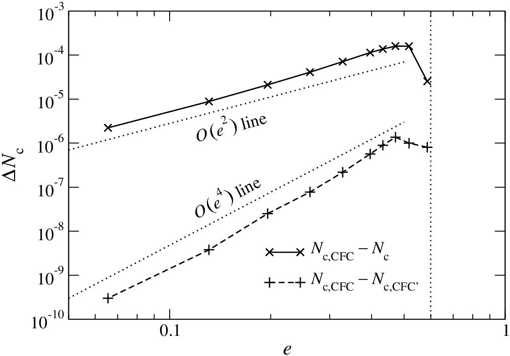
As an illustration of the above properties, we study the influence of the term in Eq. (29) when computing rotating neutron star models with a polytropic equation of state. This model setup contains the initial models used in Sec. IV. They assume axial symmetry and stationarity, in combination with rigid rotation. We build a sequence of rotating polytropes with increasing rotation frequencies, while keeping the central enthalpy fixed, which produces models of increasing masses from (no rotation), to (the Kepler limit; see below). For all these models, we use three gravitational field schemes: the exact Einstein equations using the stationary ansatz in FCF, and the two approximate ones, regular CFC and CFC, neglecting the term in Eq. (29). The results are displayed on a logarithmic scale in Fig. 5. In the top panel we show the maximal amplitudes of (relatively to ) in both FCF and regular CFC, as functions of the ellipticity defined in Eq. (47). This quantity is physically and numerically limited by the minimal rotational period at the so-called mass-shedding limit (or Kepler limit), when centrifugal forces exactly balance gravitational and pressure forces at the star’s equator. In the FCF case we plot the maximal amplitude of . This quantity is dimensionless and represents the deviation of the three-metric from conformal flatness, which can be interpreted as the relative error one makes in the metric when using CFC instead of FCF. Note that this error in computing by discarding the term in the CFC approximation is roughly of the same magnitude as the error on the metric in the CFC case. All these quantities decrease like as expected, except for stars rotating close to the Kepler limit. Indeed, the development in powers is equivalent to a slow-rotation approximation (see, e.g., [57]) by perturbing spherically symmetric configurations, and, when comparing these slow-rotation results to numerical “exact” ones for rigidly rotating stars (see, e.g., [58] in the two-fluids case), one sees that they usually agree extremely well, excepted very close to the Kepler limit, where this “perturbed spherical symmetry” approach is no longer valid. Finally, because appears as a quadratic source term in the Poisson-like equations (15) and (16), the overall errors on the lapse or the conformal factor are even smaller, as shown in the bottom panel of Fig. 5. In the case of the central value of the lapse, the error due to the CFC approximation is maximal at the Kepler limit and for the studied sequence. The error which is then due to neglecting within the CFC scheme amounts to and decreases faster than the error due to the CFC approximation, namely, as , again except near the Kepler limit. Our tests thus show that for stationary rotating neutron star models this additional approximation induces an error which falls within the overall CFC approximation.
References
- [1] J. W. York, Sources of gravitational radiation (Cambridge University Press, Cambridge, 1979), p. 83.
- [2] M. Alcubierre, Introduction to numerical relativity (Oxford University Press, Oxford, 2008).
- [3] E. Gourgoulhon, arXiv:gr-qc/0703035
- [4] J. A. Isenberg, Int. J. Mod. Phys. D 17, 265 (2008).
- [5] J. R. Wilson and G. J. Mathews, in Frontiers in numerical relativity, edited by C. R. Evans, L. S. Finn and D. W. Hobill (Cambridge University Press, Cambridge, 1989), p. 306.
- [6] H. Dimmelmeier, J. A. Font, and E. Müller, Astron. Astrophys. 393, 523 (2002).
- [7] R. Oechslin, S. Rosswog, and F.-K. Thielemann, Phys. Rev. D 65, 103005 (2002).
- [8] M. Saijo, Astrophys. J. 615, 866 (2004).
- [9] E. B. Abdikamalov, H. Dimmelmeier, L. Rezzolla, and J. C. Miller, Mon. Not. R. Astron. Soc., submitted (2008).
- [10] J. W. York Jr., Phys. Rev. Lett. 82, 1350 (1999).
- [11] H. P. Pfeiffer and J. W. York Jr., Phys. Rev. D 67, 044022 (2003).
- [12] H. P. Pfeiffer, J. Hyperbol. Diff. Equat. 2, 497 (2005).
- [13] H. P. Pfeiffer and J. W. York Jr., Phys. Rev. Lett. 95, 091101 (2005).
- [14] T. W. Baumgarte, N. O’Murchadha, and H. P. Pfeiffer, Phys. Rev. D 75, 044009 (2007).
- [15] D. Walsh, Class. Quantum Grav. 24, 1911 (2007).
- [16] N. O’Murchadha and J. W. York Jr., J. Math. Phys. 14, 1551 (1973).
- [17] N. O’Murchadha and J. W. York Jr., Phys. Rev. D 10, 428 (1974).
- [18] O. Rinne, Class. Quantum Grav. 25, 135009 (2008).
- [19] J. L. Jaramillo, J. A. Valiente Kroon and E. Gourgoulhon, Class. Quantum Grav. 25, 093001 (2008).
- [20] M. W. Choptuik, E. W. Hirschmann, S. L. Liebling, and F. Pretorius, Class. Quantum Grav. 20, 1857 (2003).
- [21] O. Rinne, PhD Thesis, University of Cambridge, UK (2005), arXiv:gr-qc/0601064.
- [22] O. Rinne and J. M. Stewart, Comm. Math. Phys. 22, 1143 (2005).
- [23] S. Bonazzola, E. Gourgoulhon, P. Grandclément, and J. Novak, Phys. Rev. D 70, 104007 (2004).
- [24] I. Cordero-Carrión, J. M. Ibáñez, E. Gourgoulhon, J. L. Jaramillo, and J. Novak, Phys. Rev. D 77, 084007 (2008).
- [25] V. Moncrief, L. Buchman, H. P. Pfeiffer, O. Rinne, and O. Sarbach, talk at From geometry to numerics workshop, Institut Henri Poincaré, Paris (2006), www.luth.obspm.fr/IHP06/workshops/geomnum/, and private communication.
- [26] J. R. Wilson, G. J. Mathews, and P. Marronetti, Phys. Rev. D 54, 1317 (1996).
- [27] J. L. Jaramillo, M. Ansorg, and F. Limousin, Phys. Rev. D 75, 024019 (2007).
- [28] H. Dimmelmeier, J. Novak, J. A. Font, J. M. Ibáñez, and E. Müller, Phys. Rev. D 71, 064023 (2005).
- [29] C. D. Ott, H. Dimmelmeier, A. Marek, H.-T. Janka, I. Hawke, B. Zink, and E. Schnetter, Phys. Rev. Lett. 98, 261101 (2007).
- [30] P. Cerdá-Durán, J. A. Font, and H. Dimmelmeier, Astron. Astrophys. 474, 169 (2007).
- [31] G. B. Cook, S. L. Shapiro, and S. A. Teukolsky, Phys. Rev. D 53, 5533 (1996).
- [32] H. Dimmelmeier, N. Stergioulas, J. A. Font, Mon. Not. R. Astron. Soc. 368, 1609 (2006).
- [33] R. Oechslin, H.-T. Janka, and A. Marek, Astron. Astrophys. 467, 395 (2007).
- [34] J. A. Faber, P. Grandclément, and F. A. Rasio, Phys. Rev. D 69, 124036 (2004).
- [35] F. Banyuls, J. A. Font, J. M. Ibáñez, J. M. Martí, and J. A. Miralles, Astrophys. J. 476, 221 (1997).
- [36] J. A. Font, J. Phys. Conf. Ser. 91, 012002 (2007).
- [37] M. Taylor, Partial differential equations III. Nonlinear equations (Applied Mathematical Sciences, Springer-Verlag, New York, 1996).
- [38] L. C. Evans, Partial differential equations (American Mathematical Society, Providence, 1998).
- [39] M. Protter and H. Weinberger, Maximum principles in differential equations (Prentice-Hall, Englewood Cliffs, 1967).
- [40] H. Komatsu, Y. Eriguchi, and I. Hachisu, Mon. Not. R. Astron. Soc. 237, 335 (1989).
- [41] N. Stergioulas and J. L. Friedman, Astrophys. J. 444, 306 (1995).
- [42] S. Bonazzola, E. Gourgoulhon, M. Salgado, and J. A. Marck, Astron. Astrophys. 278, 421 (1993).
- [43] S. L. Shapiro and S. A. Teukolsky, Astrophys. J. 235, 199 (1980).
- [44] A. Lichnerowicz, J. Math. Pures Appl. 23, 37 (1944); reprinted in A. Lichnerowicz, Choix d’œuvres mathématiques (Hermann, Paris, 1982), p. 4.
- [45] M. Shibata and K. Uryū, Phys. Rev. D 74, 121503(R) (2006); Class. Quantum Grav. 24, S125 (2007).
- [46] H. Dimmelmeier, J. A. Font, and E. Müller, Astron. Astrophys. 388, 917 (2002).
- [47] L. Baiotti, I. Hawke, P. J. Montero, F. Löffler, L. Rezzolla, N. Stergioulas, J. A. Font, and E. Seidel, Phys. Rev. D 71, 024035 (2005).
- [48] L.-M. Lin and J. Novak, Class. Quantum Grav. 23, 4545 (2006).
- [49] http://www.lorene.obspm.fr/
- [50] L.-M. Lin and J. Novak, Class. Quantum Grav. 24, 2665 (2007).
- [51] J. A. Font, T. Goodale, S. Iyer, M. Miller, L. Rezzolla, E. Seidel, N. Stergioulas, W.-M. Suen, and M. Tobias, Phys. Rev. D, 65, 084024 (2002).
- [52] A. Marek, H. Dimmelmeier, H.-T. Janka, E. Müller, and R. Buras, Astron. Astrophys. 445, 273 (2006).
- [53] A. Garat and R. H. Price, Phys. Rev. D 61, 124011 (2000).
- [54] D. Garfinkle and G. C. Duncan, Phys. Rev. D 63, 044011 (2001).
- [55] P. Cerdá-Durán, G. Faye, H. Dimmelmeier, J. A. Font, J. M. Ibáñez, E. Müller, and G. Schäfer, Astron. Astrophys. 439, 1033 (2005).
- [56] W. Kley and G. Schäfer, Phys. Rev. D 60, 027501 (1999).
- [57] J. B. Hartle and K. S. Thorne, Astrophys. J. 153, 807 (1968).
- [58] R. Prix, J. Novak and G. L. Comer, Phys. Rev. D 71, 043005 (2005).