1A closed trapped surface we want to construct. The vertical coordinate is = t - v r , while the horizontal one is r . One dimension has been suppressed, and the 2-surface appears as a curve. The Vaidya region has been shrunk to a very thin shell, causing the trapped curve to have kinks as it passes through it.

September 2008

A NOTE ON TRAPPED SURFACES

IN THE VAIDYA SOLUTION

Ingemar Bengtsson¹¹ 1 Email address: ingemar@physto.se. Supported by VR.

Stockholms Universitet, Fysikum
AlbaNova
S-106 91 Stockholm, Sweden

José M. M. Senovilla²² 2 Email address: josemm.senovilla@ehu.es. Supported by grants FIS2004-01626 (MEC) and GIU06/37 (UPV/EHU)

Física Teórica, Universidad del País Vasco
Apartado 644
48080 Bilbao, Spain

Abstract

The Vaidya solution describes the gravitational collapse of a finite shell of incoherent radiation falling into flat spacetime and giving rise to a Schwarzschild black hole. There has been a question whether closed trapped surfaces can extend into the flat region (whereas closed outer trapped surfaces certainly can). For the special case of self-similar collapse we show that the answer is yes, if and only if the mass function rises fast enough.

1. Introduction

What is a black hole? A possible answer is that a black hole is a region of an asymptotically flat spacetime bounded by an event horizon. Because the event horizon has a teleological character—it can be located only when the full solution is known—other answers have been sought [1, 2, 3]. They rely on the occurence of trapped surfaces in the interior. A possible “boundary” of the black hole region might be a dynamical horizon, a spacelike hypersurface foliated by marginally trapped surfaces and typically lying well inside the event horizon. But there are difficulties with such a definition too. Here it seems pertinent to ask for the boundary of the region of spacetime through which closed trapped surfaces pass. It was conjectured by Eardley that a closed outer trapped surface passes through every point interior to the event horizon [4], but if the surfaces are required to be genuinely trapped the corresponding statement is not true in general [5]. The boundary we ask for will lie somewhere in between a dynamical horizon and the event horizon (unless these coincide, as they do in the stationary case).

In this note we address a very concrete question. Consider the spherically symmetric Vaidya solution [6, 7]

ds^{2}=-\left(1-\frac{2m(v)}{r}\right)dv^{2}+2dvdr+r^{2}d\theta^{2}+r^{2}\sin^{2}{\theta}d\phi^{2}\ .

(1)

Einstein’s equations read

G_{ab}=8\pi T_{ab}=\frac{2\dot{m}}{r^{2}}l_{a}l_{b}\ ,\hskip 28.45274ptl_{a}=-\nabla_{a}v\ .

(2)

Thus $l_{a}$ is a null vector field, and the energy-momentum tensor is that of a radiation fluid. The energy conditions are obeyed provided that $\dot{m}\geq 0$ , where the dot denotes differentiation with respect to $v$ . But otherwise the rate at which radiation comes in is at our disposal. A simple choice, leading to a self-similar spacetime, is [8]

m=\left\{\begin{array}[]{cll}0&,&v\leq 0\\ \mu v&,&0\leq v\leq M/\mu\\ M&,&v\geq M/\mu\end{array}\right.\ .

(3)

This describes a finite shell of radiation entering flat spacetime from past null infinity, ending in a vacuum Schwarzschild black hole when the inflow stops.

For the Vaidya solution Ben-Dov has shown that Eardley’s conjecture is true [5]. However, this result concerns outer trapped surfaces, that is closed spacelike 2-surfaces whose outer null expansion is negative. For trapped surfaces, having both null expansions negative, Ben-Dov was able to show that there is a region of flat spacetime, inside the event horizon, into which no closed trapped surface can extend. The question whether closed trapped surfaces are able to extend into any part of the flat region was left open, and numerical investigations have so far not settled it [9]. We will now proceed to answer this question for the special case of self-similar collapse. In a companion paper we discuss the issues in greater generality [10].

2. Basic facts

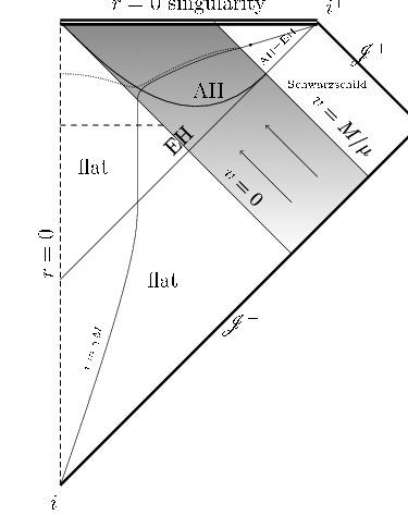
The solution is shown as a Penrose diagram in Fig. 4 (where it has been decorated with some extra structures to be encountered as we go on). Note that the part of flat space lying inside the black hole is a causal diamond: it is the intersection of the interior of two light cones, the event horizon and the inner part of the dust shell. The proper length of the geodesic connecting their vertices represents the maximum time an observer can live in this region, and will be calculated in eq. (23).

The curved region certainly contains closed trapped surfaces. The round spheres $r=$ constant, $v=$ constant are trapped if and only if $r<2m(v)$ . Hence there is an apparent horizon at

r=2m\hskip 14.22636pt\Longleftrightarrow\hskip 14.22636ptx\equiv\frac{v}{r}=\frac{1}{2\mu}\ .

(4)

Note the introduction of the variable $x$ , which is a convenient one to use in the self-similar Vaidya region. In the Vaidya region the apparent horizon is a spacelike hypersurface, and in fact a dynamical horizon. In the self-similar case it is intrinsically flat, and the trace of its extrinsic curvature is

K=\frac{1-8\mu}{8v\mu^{3/2}}\ .

(5)

We know that a naked singularity will occur if and only if $\mu\leq 1/16$ [8, 11]. Intuitively, the infinite mass density that would occur in a flat background becomes clothed only if the mass function rises fast enough, and we will assume that it does. Thus we study genuine black hole spacetimes without naked singularities, and it is our aim to construct closed trapped surfaces entering the flat region.

We will need the null expansions for some special 2-surfaces. We quote them in a form that applies to any choice of the mass function. First we consider the 2-surfaces

\phi=\varphi\hskip 19.91692pt\theta=\frac{\pi}{2}\hskip 19.91692ptr=R(\rho)\hskip 19.91692ptv=V(\rho)\ .

(6)

The first fundamental form is

d\gamma^{2}=\Delta d\rho^{2}+R^{2}d\varphi^{2}\ ,\hskip 22.76219pt\Delta\equiv V^{\prime}\left[2R^{\prime}-\left(1-\frac{2m}{R}\right)V^{\prime}\right]\ ,

(7)

where the prime stands for differentiation with respect to $\rho$ . For spacelike 2-surfaces we demand $\Delta>0$ , hence we must have $V^{\prime}\neq 0$ . It follows that $R^{\prime}=0$ can occur only inside the apparent horizon. Normal vectors to the 2-surfaces include

n=\frac{1}{\sqrt{\Delta}}(-R^{\prime}dv+V^{\prime}dr)\ ,\hskip 14.22636pte=Rd\theta\ ;\hskip 22.76219pt-n^{2}=e^{2}=1\ ,\hskip 11.38109ptn\cdot e=0\ .

(8)

The corresponding null normals are

k_{\pm}=n\pm e\ .

(9)

The null expansions are

\theta_{\pm}=\frac{1}{2\sqrt{\Delta}}\left[\frac{1}{\Delta}\left(R^{\prime}V^{\prime\prime}-V^{\prime}R^{\prime\prime}+\frac{m}{R^{2}}R^{\prime}V^{\prime 2}-\frac{\dot{m}}{R}V^{\prime 3}\right)-\frac{R^{\prime}}{R}+\frac{V^{\prime}}{R}(1-\frac{m}{R})\right]

(10)

and they are equal to each other.

We will also consider the 2-surfaces

\phi=\varphi\hskip 19.91692pt\theta=\Theta(\rho)\hskip 19.91692ptr=r_{0}\hskip 19.91692ptv=V(\rho)\ .

(11)

The first fundamental form is

d\gamma^{2}=\Delta d\rho^{2}+r_{0}^{2}d\varphi^{2}\ ,\hskip 22.76219pt\Delta\equiv\left(\frac{2m}{r_{0}}-1\right)V^{\prime 2}+r_{0}^{2}\Theta^{\prime 2}\ ,

(12)

and again we demand $\Delta>0$ . We assume that we are inside the apparent horizon, in which case normal vectors to the 2-surfaces include

n=\frac{1}{\sqrt{\frac{2m}{r}-1}}dr\hskip 28.45274pte=\frac{r\sqrt{\frac{2m}{r}-1}}{\sqrt{\Delta}}\left(V^{\prime}d\theta-\Theta^{\prime}dv-\frac{\Theta^{\prime}}{\frac{2m}{r}-1}dr\right)\ .

(13)

Again the null normals are given by $k_{\pm}=n\pm e$ . The null expansions are

	$\displaystyle\theta_{\pm}=\frac{\sqrt{\frac{2m}{r}-1}}{2\Delta^{\frac{3}{2}}}\times\hskip 204.85983pt$

	$\displaystyle\times\Big[\pm r(\Theta^{\prime}V^{\prime\prime}-V^{\prime}\Theta^{\prime\prime})+\frac{\sqrt{\Delta}}{r}\left((V^{\prime 2}(1-\frac{m}{r})-2r^{2}\Theta^{\prime 2}\right)\pm\frac{\Delta V^{\prime}}{r}\cot{\Theta}\Big]$		(14)

	$\displaystyle-\frac{1}{\sqrt{\frac{2m}{r}-1}}\frac{1}{\Delta^{\frac{3}{2}}}(\sqrt{\Delta}\mp r\Theta^{\prime})\frac{\dot{m}}{r}V^{\prime 2}\ .$

In the Schwarzschild region $\dot{m}=0$ , and the last term vanishes.

3. Plan

The idea behind the construction to follow is simple. We start with a trapped surface in the flat region, say a hyperboloid “bending down in time”. Topologically this is an open disk. It passes through the origin in flat space, and meets the shell of radiation in a circle. In the Schwarzschild region as well we can find a trapped surface meeting the shell in a circle, say the cylindrical 2-surface

r=\mbox{constant}<M\ ,\hskip 28.45274pt\theta=\frac{\pi}{2}\ .

(15)

By means of either eq. (10) or eq. (14) we can check that this cylinder does have both null expansions negative (and it will be marginally trapped if $r=M$ ). Now we must do two things: we must interpolate between these two surfaces in the Vaidya region, and we must “cap” the cylinder to ensure that the surface becomes closed. For the last part our idea is to join the cylinder to a hemispherical cap; whether this can be done while keeping both null expansions negative will be decided by eq. (14). Fig. 1 clarifies our plan.

Refer to caption — Figure 1: A closed trapped surface we want to construct. The vertical coordinate is $t=v-r$ , while the horizontal one is $r$ . One dimension has been suppressed, and the 2-surface appears as a curve. The Vaidya region has been shrunk to a very thin shell, causing the trapped curve to have kinks as it passes through it.

4. A family of trapped surfaces in the flat and Vaidya region

In flat space we obtain a marginally trapped (but not closed!) surface by setting $\theta=\pi/2$ and $t=$ constant, where $t=v-r$ . We obtain a family of trapped surfaces of this type by choosing the hyperboloids

(t-t_{0})^{2}-r^{2}=k^{2}\ ,\hskip 19.91692ptt=t_{0}-\sqrt{r^{2}+k^{2}}\ ,\hskip 19.91692ptt_{0}<k\ .

(16)

The expansions are

H(k_{\pm})=-\frac{2}{k}\ .

(17)

In a $v-r$ -diagram these surfaces obey

0<\frac{dv}{dr}<1\ .

(18)

In particular they meet the Vaidya region—at $v=0$ —with a slope that is less than one, but otherwise arbitrary.

The Vaidya region requires more care. The surface will be defined by eqs. (6), with

R=\rho\ ,\hskip 28.45274pt\frac{dV}{dR}=\frac{a}{b-X}\ ,\hskip 14.22636ptX\equiv\frac{V}{R}\ .

(19)

Here $a$ and $b$ are positive real numbers at our disposal. The differential equation can be solved straightforwardly [11, 10], if we rewrite it as

R\frac{dX}{dR}=\frac{(X-\frac{b}{2})^{2}+\Lambda^{2}}{b-X}\ ,\hskip 22.76219pt\Lambda^{2}\equiv a-\frac{b^{2}}{4}\ .

(20)

To ensure that the solution has the properties we want it to, we choose

\Lambda^{2}=a-\frac{b^{2}}{4}>0\hskip 14.22636pt\Leftrightarrow\hskip 14.22636pt4\frac{a}{b}>b\ .

(21)

In particular this condition ensures that the first and second derivatives have the same sign,

\frac{d^{2}V}{dR^{2}}=\frac{1}{a^{2}R}\left(\frac{dV}{dR}\right)^{3}\left(\left(X-\frac{b}{2}\right)^{2}+a-\frac{b^{2}}{4}\right)\ .

(22)

In the $v-r$ -diagram the curve becomes vertical at $X=b$ . A look at Fig. 2 may be helpful here.

We note in passing that radial null geodesics are given by the same differential equation (19), with $a=1/\mu$ , $b=1/2\mu$ . This allows us to locate the event horizon, and also to calculate the maximum time $\Delta t$ an observer can live in the flat region inside the black hole. This lifetime grows with $M$ , and equals

\Delta t=4M\exp\left\{-\frac{2}{\sqrt{16\mu-1}}\arctan\frac{1}{\sqrt{16\mu-1}}\right\}<4M\ .

(23)

Thus, the larger the rate $\mu$ the sooner the event horizon starts to develop.

The surface we have defined must be matched properly to trapped surfaces in the flat and Schwarzschild regions. To ensure that it matches to a trapped hyperboloid in the flat region we require

\left.\frac{dV}{dR}\right|_{X=0}<1\hskip 14.22636pt\Rightarrow\hskip 14.22636pt\frac{a}{b}<1\ .

(24)

This ensures that the first derivative can be made continuous. There will be a finite jump in the second derivative. We will accept this, although in the end the construction can be made smoother, should one insist on it. The Schwarzschild region begins at $V=M/\mu$ . At this boundary we want to join our surface to a trapped cylinder with $R=\gamma M$ , where $\gamma<1$ . The curve is now vertical ( $X=b$ ), so the requirement becomes

b=\frac{1}{\gamma\mu}\ .

(25)

Again this ensures that first derivatives are continuous. But now we have imposed a restriction on the mass function, namely

\mu=\frac{1}{\gamma b}>\frac{b}{4a\gamma}>\frac{1}{4\gamma}\ .

(26)

Recall that $b/a>1$ and $\gamma<1$ . In the next section we will see that we must impose a somewhat stronger condition on $\gamma$ when we “cap” the surface in the Schwarzschild region. In the final section we observe that a restriction on $\mu$ of roughly this order can be deduced on general grounds, so the fact that such a restriction arises is not an artefact of the special way in which we construct the closed trapped surface.

We must ensure that our surface is spacelike. This will be so if $\Delta>0$ in eq. (7), and given $b>a$ this holds for all $X$ provided that

a\geq\frac{1}{\mu}\ .

(27)

This is unproblematic. Finally we must check that the surface is indeed trapped. A calculation starting from eq. (10) shows that the null expansions are given by

\theta_{\pm}=-N\left[(a\mu-1)\left(a+3(b-a)X+(2a\mu-1)X^{2}\right)+(b-a)(2b-a)\right]

(28)

where

N=\frac{1}{2r\sqrt{a}}\frac{1}{(2b-a+2(\mu a-1)X)^{3/2}}\ .

(29)

With the conditions already imposed the expansions are indeed negative, and we are done.

One additional detail is worth giving: Suppose the surface enters the Schwarzschild region at $r=r_{S}$ . Then it enters the Vaidya region from flat space at

r_{0}=r_{S}\ \mbox{exp}\left[-\frac{b}{\Lambda}\arctan{\frac{b}{2\Lambda}}\right]\ .

(30)

This follows [10] from the explicit solution of eq. (20).

To summarize, we have found a trapped surface that begins as a piece of a hyperboloid (say) in Minkowski space, continues through the Vaidya region, and joins the trapped cylinders at $r<M$ in the Schwarzschild region. It is depicted in Fig. 2. But it is still not a closed surface. Two minor comments: The surface is only $C^{2-}$ , but making it smoother presents no real difficulty. It is marginally trapped if $a=b=1/\mu$ , and if the hyperboloid is replaced by a plane in the flat region.

5. Closing the trapped surfaces in the Schwarzschild region

We are now safely in the Schwarzschild region, and our surface is joined to a cylinder at $r=\gamma M$ , $\gamma<1$ . We must add a hemispherical cap to it. This piece of the surface will be of the form (11), with $V=\rho$ . The surface is in effect described by a curve in the $\Theta-V$ -plane, see Fig. 3. The null expansions are given by eq. (14), and we can bring this to slightly more manageable form by introducing the dimensionless variable $\sigma$ ,

\sigma=V/\gamma M-\sigma_{0}\ ,

(31)

where $\sigma_{0}$ is a constant we can adjust so that we start “bending” the curve at $\sigma=0$ . Let $\dot{\Theta}$ be the derivative of $\Theta$ respect to $\sigma$ , and assume that

\cot{\Theta}\geq 0\ ,\hskip 34.1433pt\ddot{\Theta}\leq 0\ .

(32)

A calculation now shows that both null expansions will be negative if and only if

2\dot{\Theta}^{2}+\frac{1}{\gamma}-1>\sqrt{\frac{2}{\gamma}-1+\dot{\Theta}^{2}}\left(\cot{\Theta}-\frac{\ddot{\Theta}}{\frac{2}{\gamma}-1+\dot{\Theta}^{2}}\right)\ .

(33)

Our “initial data” are $\Theta=\pi/2$ , $\dot{\Theta}=0$ at $\sigma=0$ . We have not been able to handle the inequality in general. Let us just remark that as soon as a negative second derivative develops, there will be restrictions on $\gamma$ stronger than the condition $\gamma<1$ that we have already imposed.

A simple choice of the function $\Theta(\sigma)$ , leading to a curve with continuous first derivatives, is to take a quadrant of the circle

\left(\Theta-\frac{\pi}{2}+\delta\right)^{2}+\sigma^{2}=\delta^{2}\ ,\hskip 22.76219pt0<\delta\leq\frac{\pi}{2}\ .

(34)

This joins the initial cylinder to a portion of one of the standard trapped round spheres at $\sigma=\mbox{constant}>0$ . At $\sigma=0$ the trapping condition (33) is obeyed provided that

\sqrt{\frac{2}{\gamma}-1}\left(\frac{1}{\gamma}-1\right)>\frac{1}{\delta}\ .

(35)

Hence

\delta=\frac{\pi}{2}\hskip 14.22636pt\Rightarrow\hskip 14.22636pt\gamma<0.68514\ .

(36)

We have checked numerically that with this restriction the inequality (33) is obeyed for all $0\leq\sigma\leq\pi/2$ , so this does it: we do have a closed trapped surface that begins in the flat region and ends in Schwarzschild. Topologically it is a 2-sphere.

Clearly the construction can be improved by changing the precise shape of the curve in the $\Theta-V$ -plane. The best we were able to do (using a segment of an ellipse rather than a segment of a circle) was $\gamma<0.75$ . Another possibility would perhaps be to start “capping” the surface already in the Vaidya region, but we have not considered this.

6. Discussion

In the self-similar Vaidya solution we have constructed closed trapped surfaces that begin in the flat region, pass through the shell, and end in the Schwarzschild region. See Fig. 4.

The mass function is given by eq. (3) and the construction works provided that

\mu>\frac{1}{0.68}\frac{1}{4}\ .

(37)

On the other hand we know from the companion paper [10], using an argument based on the interplay between the Kerr-Schild vector field [12] and the trapped surfaces, that it is impossible to construct a closed trapped surface entering the flat region if

\mu\leq\frac{1}{8}\ .

(38)

It will be observed that there is a gap between these two results.

Indeed our construction is not optimal. We indicated a way in which the number $0.68$ in inequality (37) can be increased somewhat. It must however be kept smaller than one for the kind of surface we consider. We do not know what one can achieve if one gives up axial symmetry of the surfaces, say. On the other hand we do know that the inequality (38), which rules out closed trapped surfaces extending into the flat region, can be relaxed. The true limit must lie somewhere in between.

Like Ben-Dov’s construction of closed outer trapped surfaces [5], our result serves to underline the fact that the teleological character of event horizons has a translation into a “non-local” property of closed trapped surfaces. They can live partly in a region of spacetime whose entire past is flat, if energy falls across them elsewhere to make their closure possible.

Acknowledgements

We thank Jan Åman for performing some checks. José M.M. Senovilla thanks the Physics Department at Stockholm University for its hospitality; we both thank the Wenner-Gren Foundation for making his visit possible.

References

[1] S. A. Hayward, Black holes: New horizons, in V. G. Gurzadyan et al. (eds.): Proc. of the Ninth Marcel Grossmann meeting, World Scientific 2002.
[2] A. Ashtekar and B. Krishnan, Isolated and dynamical horizons and their applications, Living Rev. Rel. 7, 10 (2004).
[3] I. Booth, Black hole boundaries, Can. J. Phys. 83 (2005) 1073.
[4] D. M. Eardley, Black hole boundary conditions and coordinate conditions, Phys. Rev. D57 (1998) 2299.
[5] I. Ben-Dov, Outer trapped surfaces in Vaidya spacetime, Phys. Rev. D75 (2007) 064007.
[6] P. C. Vaidya, The gravitational field of a radiating star, Proc. Indian Acad. Sci. A33 (1951) 264.
[7] P. C. Vaidya, ’Newtonian’ time in general relativity, Nature 171 (1953) 260.
[8] W. A. Hiscock, L. G. Williams and D. M. Eardley, Creation of particles by shell-focusing singularities Phys. Rev. D26 (1982) 751
[9] E. Schnetter and B. Krishnan, Non-symmetric trapped surfaces in the Schwarzschild and Vaidya spacetimes, Phys. Rev. D73 (2006) 021502(R).
[10] I. Bengtsson and J. M. M. Senovilla, The boundary of the region with trapped surfaces in spherical symmetry, to appear.
[11] A. Papapetrou, Formation of a singularity and causality, in N. Dadhich et al. (eds.): A Random Walk in Relativity and Cosmology, Wiley 1985.
[12] B. Coll, S. R. Hildebrandt and J. M. M. Senovilla, Kerr-Schild symmetries, Gen. Rel. Grav. 33 (2001) 649.